Chern-number spin Hamiltonians for magnetic nano-clusters by DFT methods

Abstract

Combining field-theoretical methods and ab-initio calculations, we construct an effective Hamiltonian with a single giant-spin degree of freedom, capable of the describing the low-energy spin dynamics of ferromagnetic metal nanoclusters consisting of up to a few tens of atoms. In our procedure, the magnetic moment direction of the Kohn-Sham SDFT wave-function is constrained by means of a penalty functional, allowing us to explore the entire parameter space of directions, and to extract the magnetic anisotropy energy and Berry curvature functionals. The average of the Berry curvature over all magnetization directions is a Chern number - a topological invariant that can only take on values equal to multiples of one half, representing the dimension of the Hilbert space of the effective spin system. The spin Hamiltonian is obtained by quantizing the classical anisotropy energy functional, after performing a change of variables to a constant Berry curvature space. The purpose of this article is to examine the impact of the topological effect from the Berry curvature on the low-energy total-spin-system dynamics. To this end, we study small transition metal clusters: Co_n ($n=2,...,5$), Rh₂, Ni₂, Pd₂, Mn_xN_y, Co₃Fe₂.

2007 Volume number Issue number identifier

I Introduction

The present interest in magnetic nanoparticles, nano-clusters and molecular magnetsSellmyer and Skomski (2006); Gatteschi et al. (2006) is partly motivated by the quest for nano-scale information storage devicesSun et al. (2000), and by possible applications in nano-spintronics and quantum computation devices. Most of the advances achieved in the last few years in this field have been fueled by the remarkable experimental ability to synthesize, manipulate and characterize these systems at the atomic scaleSellmyer and Skomski (2006). Theoretical work, based on refined modelsFélix-Medina et al. (2003); Cehovin et al. (2002); Skomski (2003) and advanced computational toolsEber et al. (2005); Kashyap et al. (2006), is also providing crucial understanding and new predictions. Magnetic metal nano-clusters, like other magnetic nanostructures, typically display enhanced magnetic propertiesBillas et al. (1994) and many novel classical and quantum phenomena, which challenge our understanding of magnetismXu et al. (2005); Tiago et al. (2006).

A quantity that is the topic of intense interest in nanomagnetism, is the magnetic anisotropy. This is the dependence of the total energy of the system on the orientation direction of the magnetic moment. The presence of two or more stable orientations in the anisotropy energy functional, separated by an energy barrier, is the crucial property exploited in information storage devices. The origin of Magnetocrystalline Anisotropy Energy (MAE) in magnetic materials is subtle, being a relatively small effect arising primarily from the spin-orbit interaction. It is now possible to investigate experimentally the MAE in individual magnetic nanoparticlesJamet et al. (2001) and nano-clustersGambarella et al. (2003) with unprecedented accuracy. Typically the MAE in these magnetic nanostructures is found to be larger than in bulk. Gambardella et al.Gambarella et al. (2002) found that monoatomic Co chains on a stepped Pt(111) surface are ferromagnetic and have a MAE that is one-order of magnitude larger than bulk Co. Understanding the reasons of this enhancement and how to increase it further is one of the goals of ongoing research. Recent theoretical work predicts that the MAE in unsupported 4d transition metal (TM) chainsMokrousov et al. (2006) and dimersStrandberg et al. (2007) have giant MAE up to 50 meV.

Another topic of great importance, connected to the MAE and equally intensively investigated, is the spin dynamics of the collective magnetization orientation degree of freedom in single-domain nanoparticles. For a nanoparticle containing several thousand atoms, the magnetic orientation degree of freedom is a classical variable that oscillates around one energy minimum of the MAE or switches between two of them by thermal activation. Thermal switching in individual superparamagnetic nanoparticle has been recently studied by spin-polarized scanning tunneling microscopeBode et al. (2004). When the nanocluster is sufficiently small, the quantum behavior of the collective spin becomes important. The crossover from classical to quantum behavior for the magnetization collective variable is a complex problem of great scientific interest. The physical systems on which research has focused so far in studying this question are molecular magnets in a crystalGunther and Barbara (1995); Chudnovsky and Tejada (1998); Gatteschi et al. (2006). These systems contain about 100 atoms per particle, are insulators and behave like a single microscopic quantum spin, e.g. $S=10$ for Mn₁₂ acetate. Quantum effects are clearly discernible in their low-temperature relaxation properties. A large amount of literature has been devoted to studying these systemsGatteschi et al. (2006). Similar studies of the quantum spin dynamics in engineered magnetic metal nanoclusters have just begun. In a recent key experiment, Hirjibehedin et al.Hirjibehedin et al. (2006) investigated collective spin excitations in individual scanning tunnel microscope (STM)-engineered linear chains of 1 to 10 manganese atoms, by means of inelastic electron tunneling spectroscopy. Spin excitations that change both the total collective spin and the spin orientation were observed.

On the theoretical front, the microscopic description of quantum spin excitations in magnetic metal clusters is more challenging than in insulating molecular magnets, since in the metal clusters these excitations are intertwined with electronic particle-hole excitations. The need to include the crucial spin-orbit interactions adds to the complexity of the task. However, in a paper published a few years agoCanali et al. (2003), two of us put forward the idea that, for ultra-small metal clusters, where the single-particle energy level spacing is typically larger than then total MAE barrier, the ”fast” (high-energy) electronic degrees of freedom can be integrated out. It is then still possible to describe the “slow” (low-energy) dynamics of the collective magnetization orientation in terms of a single quantum mechanical giant spin $J$ only, like in molecular magnets. When spin-orbit interactions are neglected, the ground state of a magnetic nano-cluster will tend to have a large total spin quantum number $S$, and may have additional orbital degeneracies $g_{orb}$ as well. In the atomic limit for example, the ground state is characterized by total spin and total orbital angular momentum $L$ quantum numbers so that $g_{orb}=2L+1$. In clusters, orbital symmetries are reduced and $g_{orb}$ will tend to be small - in the simplest cases equal to $1$. In this case, we identify the giant spin $J$ with $S$. When spin-orbit interactions are included, this large ground state degeneracy will be lifted. Following Ref. Canali et al., 2003, the approach we take in this paper assumes that the magnetic nano-cluster has a well-defined group of low-lying energy levels which can be identified with the magnetic moment orientation degree-of-freedom. For a nano-cluster with total giant spin $J$, $2J+1$ many-body states will lie in this group. For atoms, for example, Hunds third rule states that $J=L\pm S$. The spectrum of these levels is described by a giant spin low-energy effective Hamiltonian which is the quantum generalization of the magnetic anisotropy energy.

When integrated out, the fast electronic degrees of freedom produce a Berry phase term in the effective action that can profoundly modify the behavior of the magnetization orientation degree of freedom. Indeed in this approach, orbital contributions, arising from spin-orbit interactions, are automatically included via the Berry phase term. The giant-spin of the formalism is a topological half-integer invariant known as Berry phase Chern number, which characterizes the topologically non-trivial dependence of the nano-cluster’s many-electron wave functions on magnetization orientation.

The purpose of this paper is to carry out the procedure suggested in Ref. Canali et al., 2003 by calculating Berry phase Chern numbers and extracting effective spin Hamiltonians for a variety of realistic magnetic nanoclusters containing different transition metals. In order to carry out this procedure, we calculate the MAE for all these systems. We treat the many-body electronic problem using state-of-the-art numerical methods based on Spin-Density Functional Theory (SDFT). For transition metals having the largest MAE such as Cobalt, our procedure is in principle valid for clusters containing up to hundred atoms. However, with current state-of-the-art plane wave SDFT codes and the advantages of parallel processing, the computational load sets our estimated upper limit at a few tens of atoms. Here we investigate unsupported ultra-small clusters with no more than 5 TM atoms. We neglect non-collinear spin configurations and limit ourselves to coherent magnetization solution, although we allow the possibility of both ferromagnetic and antiferromagnetic order parameters. We focus, in particular, on the challenging situation, quite ubiquitous in metal clusters, where the HOMO-LUMO gap vanishes. This is the case where the Berry phase contribution is crucial. By comparing our treatment with the ordinary procedure of extracting spin Hamiltonians from the MAE functional, where the Berry phase term is neglected, we show that the latter can lead to incorrect results for the thickness of the magnetic anisotropy energy and for the oscillation frequencies of the magnetization orientation degree of freedom.

The paper is organized as follows. In section II we give a short description of the theoretical background and the technical details needed to understand the output of the model. We then present our main results in section III and proceed with a more in-depth analysis of the different systems in section IV. Finally, we summarize our conclusions in section V.

II Theory

II.1 The Berry curvature and the Chern number

The fundamental origin of the Berry phase Berry (1984) is some parametrization of a given term in the Hamiltonian, representing a coupling to the external world It is this parametrization that leads to an observable which cannot be cast into the form of an Hermitian operator, but is instead given in terms of a phase change in the systems wavefunction. In the systems we are interested in, this parameter is the orientation of the coherent magnetization direction of the magnetic cluster, represented by the unit vector $\hat{n}$. The dependence of the many-body wavefunction on the unit vector $\hat{n}$ gives rise to the Berry phase. In its most fundamental form, the phase change in the ground state wavefunction as we vary the magnetization between points $1$ and $2$ is given by

$$\Delta\varphi_{12}=-\text{Im}\log\langle\Psi(\hat{n}_{1})|\Psi(\hat{n}_{2})\rangle\equiv-\text{Im}\log\langle 1|2\rangle,$$ (1)

which is an arbitrary phase that can be gauged away. By closing the loop in traversing the vertices of a triangle we obtain a non-vanishing phase change: $-$Im$~{}\log\langle 1|2\rangle\langle 2|3\rangle\langle 3|1\rangle$. In the continuum limit of a discrete, closed path $\gamma$ we obtain the usual definition of the Berry phase

$$\mathcal{P}=i{\displaystyle\oint\nolimits_{\gamma}}d\hat{n}\cdot\langle\Psi|\mathbf{\nabla}_{\hat{n}}\Psi\rangle.$$ (2)

If we then convert the line integral to a surface integral over the enclosed area, we can identify the integrand as a very convenient, gauge invariant quantity and define the Berry curvature Resta (2000); Auerbach (1994),

$$\mathcal{\vec{C}}[\hat{n}]=i\mathbf{\nabla}_{\hat{n}}\times\langle\Psi|\mathbf{\nabla}_{\hat{n}}\Psi\rangle.$$ (3)

The dimensionality of the total spin system is encoded in the dependence of the many-body wavefunction on the magnetization direction as a topological invariant called the Chern numberBohm et al. (2003), obtained by taking the average of the Berry curvature over the unit sphereCanali et al. (2003),

$$\mathcal{S}=\frac{1}{4\pi}\int_{S^{2}}\mathcal{\vec{C}}[\hat{n}]\cdot\hat{n}\;dA.$$ (4)

Below we will refer to $\mathcal{C}[\hat{n}]\equiv\mathcal{\vec{C}}[\hat{n}]\cdot\hat{n}$ as the Berry curvature. Without SOI, the $\mathcal{C}[\hat{n}]$ is constant and is trivially equal to the total spin quantum number $S$ Cehovin et al. (2003). There is no anisotropy as the magnetization direction is varied. Anisotropy comes from the coupling of electronic spin and orbital degrees of freedom via the inclusion of SOI. The dimension of the Hilbert space where the systems total effective spin resides is now the good quantum number and total angular momentum $J$, replacing $S$ as the Chern number of the system. For example, consider the case of a single Co atom: disregarding SOI, the system has a total spin of $S=\tfrac{3}{2}$ coming from the $3d$ electrons. Including SOI, we instead find a Chern number equal to $J=\frac{9}{2}$, in accordance with the ground state predicted by Hund’s rules. Of course there is no anisotropy for a single atom as it is rotationally invariant in the absence of a molecular or crystal field.

When the size and geometrical complexity of the cluster increases, determination of the total $J$ quantum number quickly becomes a highly non-trivial task. As is commonly the case, one may assume that SOI does not cause a level-crossing at the HOMO level. The dimensionality of the system can then be inferred from the total magnetic moment in the absence of SOI, after which the spin-orbit shifts can be estimated perturbationally. Adding the caveat of a dense level structure at the HOMO level, as in small transition metal clusters, there is the possibility that a spin-orbit induced level-crossing may alter the dimensionality, rendering the aforementioned reasoning specious. In the presence of SOI, one may again attempt to infer the total spin dimension from the magnetic moment, but this is a risky process as the numerical difficulties associated with its determination for TM clusters can easily cause a round-off error. By contrast, the Chern number can only take on values of multiples of one-half, resolving any ambiguity in obtaining the dimension of the total spin system.

It is useful to consider the perturbational expression for the Berry curvature. In the so-called parallel transport gaugeResta (2000) the phase of the wavefunction is kept constant as the magnetization direction is infinitesimally varied. Each infinitesimally translated state then becomes orthogonal to the previous state. This means that the wavefunction can become multiply valued and obtain a sign change as $\hat{n}$ executes a closed loop on the unit sphere. The choice of parallel transport gauge is implicitly made in the perturbational expression,

$$|\frac{\partial\Psi^{0}}{\partial n_{i}}\rangle=\sum_{m\neq 0}|\frac{\partial\Psi^{m}}{\partial n_{i}}\rangle\frac{\langle\Psi^{m}|\frac{\partial H\left(\hat{n}\right)}{\partial n_{i}}|\Psi^{0}\rangle}{E_{0}\left(\hat{n}\right)-E_{m}\left(\hat{n}\right)},$$ (5)

where we denote the ground state by $\Psi^{0}$ and the sum runs over excited states $\Psi^{m}.$ (5) can be inserted into the expression for the curvature (3) to yield

$$\hat{\mathcal{C}}[\hat{n}]=i\sum_{i=1}^{3}\sum_{m\neq 0}\frac{\langle\Psi^{0}|\frac{\partial H\left(\hat{n}\right)}{\partial n_{j}}|\Psi^{m}\rangle\langle\Psi^{m}|\frac{\partial H\left(\hat{n}\right)}{\partial n_{k}}|\Psi^{0}\rangle}{\left[E_{0}\left(\hat{n}\right)-E_{m}\left(\hat{n}\right)\right]^{2}}\hat{n}_{i}\;\varepsilon_{ijk}.$$ (6)

Although this equation does no service in calculating the curvature (one would have to calculate the excited states), it clearly exhibits the strong dependence of the curvature on the HOMO-LUMO gap.

II.2 Quantum Hamiltonian Extraction

We follow the procedure outlined in Canali et al. (2003) and start from an approximate imaginary-time quantum action that is a functional of the magnetization direction $\hat{n}$ of the single effective spin degree of freedom,

$$S[\hat{n}]\equiv\int d\tau\left[\langle\Psi[\hat{n}]|\mathbf{\nabla}_{\hat{n}}\Psi[\hat{n}]\rangle\cdot\frac{\partial\hat{n}}{\partial\tau}+E[\hat{n}]\right]\;.$$ (7)

The orientational degree of freedom $\hat{n}$ is more precisely defined as the direction in spin-space of the SDFT exchange-correlation effective fieldUhl et al. (1994), or its spatial average if low-energy states have non-collinear magnetization. In Eq. (7) $|\Psi[\hat{n}]\rangle$ is the Kohn-Sham single-Slater determinant ground state defined by this orientation, and $E[\hat{n}]$ is the SDFT energy. Here spin-orbit terms are included in the Hamiltonian. For simple model Hamiltonians where the exchange interaction can be decoupled by means of auxiliary field functional integrals, Eq. (7) can be derived microscopically, starting with a path integral over electronic coherent states. Eq. (7) was originally proposed by Niu and KleinmanNiu and Kleinman (1998); Niu et al. (1999) to study the spin-wave dynamics of bulk TM ferromagnets in the context of the adiabatic approximation, and successfully exploited in the actual derivation of magnon dispersion by means of density functional theoryGebauer and Baroni (2000); Bylander et al. (2000).

The Euler-Lagrange equations for extremizing the action Eq. (7) yield the semiclassical dynamics of the orientation direction $\hat{n}$,

$$\mathcal{-}iC_{\alpha\beta}[\hat{n}]\,{\dot{n}}_{\beta}+\frac{\partial E}{\partial n_{\alpha}}=0\;,$$ (8)

where the Berry curvature matrix elements $\mathcal{C}_{\alpha\beta}$ are defined as

$$\mathcal{C}_{\alpha\beta}[\hat{n}]=\frac{\partial}{\partial n_{\alpha}}\langle\Psi[\hat{n}]|\frac{i\partial}{\partial\hat{n}_{\beta}}|\Psi[\hat{n}]\rangle-\frac{\partial}{\partial n_{\beta}}\langle\Psi[\hat{n}]|\frac{i\partial}{\partial\hat{n}_{\alpha}}|\Psi[\hat{n}]\rangle\;.$$ (9)

These equations reduce to the classical Landau-Lifshitz (LL) equations when the curvature is constant and equal to the total spin moment $S$. In the presence of SOI however, the curvature is in general non-constant and can deviate considerably from $S$, particularly along directions in correspondence of which the HOMO-LUMO energy gap is small. Thus the LL equations can fail in this case. In this paper, we aimed instead at deriving a quantum mechanical description of the effective total spin, whose magnitude we identify with the Chern number $\mathcal{S}$. Equipped with the magnetic anisotropy energy and the Berry curvature functionals on the unit sphere, we can proceed with the extraction of an effective quantum Hamiltonian for this spin. Assuming that the curvature is positive definite, the low energy effective action (7) can be mapped onto that of an effective quantum spin Hamiltonian by first performing a variable transformation to constant curvature space. This Hamiltonian is a convenient tool that can be used for calculations of tunneling amplitudes, non-linear response to external fields etc. The variable transformation is given byCanali et al. (2003)

$$\phi \rightarrow\phi^{\prime}=\frac{2\pi\int_{0}^{\phi}\mathcal{C}\left(u,\phi^{\prime\prime}\right)d\phi^{\prime\prime}}{\int_{0}^{2\pi}\mathcal{C}\left(u,\phi^{\prime\prime}\right)d\phi^{\prime\prime}},$$ (10)

$$u \rightarrow u^{\prime}=-1+\frac{1}{2\pi\mathcal{S}}\int_{-1}^{u}du^{\prime\prime}\int_{0}^{2\pi}d\phi^{\prime\prime}\mathcal{C}\left(u^{\prime\prime},\phi^{\prime\prime}\right).$$ (11)

where $\mathcal{C}$ is the curvature, $\mathcal{S}$ the Chern number and $u=\cos\theta.$ This change of variables rescales the local curvature metric such that

$$\mathcal{C}\left(u,\phi\right)dud\phi=\mathcal{S}du^{\prime}d\phi^{\prime}.$$ (12)

From this expression we see that the transformed infinitesimal area element will be rescaled in order to compensate for variations in the curvature. Consequently, if $\mathcal{C}>\mathcal{S}$ the variable transform will cause an expansion of the grid points and if $\mathcal{C}<\mathcal{S}$ a contraction. At each grid point there is an energy value associated with the magnetization direction that will be relocated by the transform. In particular, we see from expression (6) that if the HOMO and the LUMO level become quasi-degenerate for one or more magnetization directions, the curvature will become quasi-singular, causing a substantial deformation of the grid.

The variable transformation allows us to rewrite the real-time action as

$$\mathcal{S}_{\text{spin}}[\hat{n}^{\prime}]\equiv\int_{0}^{t}dt^{\prime}\left[i\;\vec{A}\cdot\frac{d\hat{n}^{\prime}}{dt^{\prime}}-E\left[\hat{n}\left(\hat{n}^{\prime}\left(t^{\prime}\right)\right)\right]\right],$$ (13)

where $\vec{A}=s\hat{\phi}^{\prime}\left(1-\cos\theta^{\prime}\right)/\sin\theta^{\prime}$. This is the quantum action for a total spin of quantum number $s$, with a classical Hamiltonian $H\left[\hat{n}^{\prime}\left(t^{\prime}\right)\right]\equiv E\left[\hat{n}\left(\hat{n}^{\prime}\left(t^{\prime}\right)\right)\right]$ Auerbach (1994), that is equal to the expectation value of a quantum spin Hamiltonian $\mathcal{H}$,

$$H\left[\hat{n}^{\prime}\left(t^{\prime}\right)\right]\equiv\langle s,\hat{n}^{\prime}\left(t^{\prime}\right)|\mathcal{H}|s,\hat{n}^{\prime}\left(t^{\prime}\right)\rangle,$$ (14)

with respect to the spin coherent states $|s,\hat{n}^{\prime}\left(t^{\prime}\right)\rangle$ describing a spin $s$ parametrized by the unit vector $\hat{n}^{\prime}\left(t^{\prime}\right)$.

The quantization of the transformed magnetic anisotropy energy is then performed by expanding in spherical harmonics of highest possible order $2s$, where time-reversal symmetry precludes odd-powered harmonics from contributing.

$$E\left[\hat{n}\left(\hat{n}^{\prime}\left(t^{\prime}\right)\right)\right]=\sum_{l=0}^{2s}\sum_{m=-l}^{l}\gamma_{l}^{m}Y_{l}^{m}\left(\hat{n}^{\prime}\right)$$ (15)

The spin coherent state $|s,\hat{n}^{\prime}\left(t^{\prime}\right)\rangle$ can be constructed by applying rotation operators in the single spin-space acting on the coherent spin state with maximum polarization $m=s$. This allows us to express the RH side of (14) in terms of spherical harmonics.

$$\sum_{mm^{\prime}}\langle s,s|\mathcal{D}^{{\dagger}}\left(R\right)|s,m\rangle\langle s,m|\mathcal{H}|s,m^{\prime}\rangle\langle s,m^{\prime}|\mathcal{D}\left(R\right)|s,s\rangle$$

$$=\sum_{mm^{\prime}}\left(R_{sm}^{s}\right)^{{\dagger}}\mathcal{H}_{mm^{\prime}}^{s}R_{m^{\prime}s}^{s}$$ (16)

$$=\sum_{mm^{\prime}l\tilde{m}}\left(-1\right)^{m-s}\sqrt{4\pi\left(2l+1\right)}$$

$$\times\left(\begin{array}[c]{ccc}s&s&l\\ -s&s&0\end{array}\right)\left(\begin{array}[c]{ccc}s&s&l\\ -m&m^{\prime}&\tilde{m}\end{array}\right)Y_{l}^{\tilde{m}}\left(\hat{n}^{\prime}\right)\mathcal{H}_{mm^{\prime}}^{s}$$ (21)

where we have made use of the Wigner-Eckhart theorem and expressed the Clebsch-Gordan coefficients in terms of Wigner-3J symbols. Equating (21) to the RH side of (15), convoluting with $Y_{\lambda}^{\mu}$ and inverting, we obtain

$$H_{mm^{\prime}}^{s} =\left(-1\right)^{m^{\prime}-s}\sum_{\lambda\mu}\gamma_{\lambda}^{\mu}\sqrt{\frac{2\lambda+1}{4\pi}}$$

$$\times\left(\begin{array}[]{ccc}s&s&\lambda\\ m&-m^{\prime}&\mu\end{array}\right)\left/\left(\begin{array}[]{ccc}s&s&\lambda\\ s&-s&0\end{array}\right)\right.$$ (26)

Equation (26) is of great practical use as gives an analytical relation between the spherical harmonic expansion coefficients and the matrix elements of the quantum Hamiltonian. Once the Hamiltonian matrix has been obtained, it can be decomposed in terms of the spin operators $S_{x},$ $S_{y},$ $S_{z}$ and $S^{2}$.

II.3 Computational Details

Our numerical tool is SDFT using the Projector Augmented Waves (PAW) formalism Blochl (1994) as implemented in the VASP Kresse and Furthmuller (1996) code. As such, the method depends on representing the atoms with PAW pseudopotentials, in which the core electrons are described on an auxiliary radial grid. This method can be said to be of all electron type, although only the valence electrons participate in the full variational procedure, whereas the core region is adjusted by applying boundary and conservation conditions. The pseudopotentials are generated in the generalized gradient approximation which gives a better description of the exchange-correlation effects.

We use accurate parameter settings for our calculations. By this we mean a valence (auxiliary) energy cutoff of 348(621), 298(488), 351(709), 326(541), 381(751), 351(740), 520(815) eV in the case of Co, Rh, Ni, Pd, Fe, Mn and N, respectively. In that order, the PAW pseudopotentials Kresse and Joubert (1999) for these elements are generated in the following electronic valence configurations: $3d^{8}4s^{1}$, $4d^{8}5s^{1}$, $3d^{9}4s^{1}$, $4d^{9}5s^{1}$, $3p^{6}3d^{7}4s^{1}$, $3p^{6}3d^{6}4s^{1}$ and $2s^{2}2p^{3}$. To avoid wrap-around errors we chose a dense FFT-grid taking into account all $\vec{G}$-vectors that are twice as large as the vectors in the basis set for the valence region and the 16/3 times as large for the auxiliary region. Interaction between the periodically repeated cells is suppressed by selecting a relatively large supercell-size of $11\times 11\times 11$ A (in the case of Mn_xN_y we use elongated cells suitable for these geometries). Only the $\Gamma$-point is used in the calculations and we have monitored dispersion by comparing the eigenenergy spectrum at the $\Gamma$-point to that of the X-point, at the edge of the Brillouin zone - in general there is no or very little dispersion. By making use of the Vosko-Wilk-Nusair Vosko et al. (1980) interpolation formula for the correlation part of the exchange-correlation functional, magnetic moments and energies are enhanced. All calculations are performed in non-collinear mode (as described in ref. Hobbs et al., 2000) with and without SOI.

The calculation of electronic properties for small TM clusters is a daunting task. Well converged solutions are often obscured by a dense level structure at the HOMO level, causing sporadic jumps between different spin-configurations and in a faulty ordering of the eigenlevels. As noted by Pederson et. Al Pederson and Jackson (1991) (as well as Jamorski et al. (1997); Micherlini et al. (1998)), the use of a finite (in our case Gaussian) smearing makes it possible to achieve convergence in the self-consistent state. This fake temperature causes a decreasing fractional occupation of the levels around the HOMO level, enabling the correct ordering of eigenstates. At the end of the calculation, the limit of zero smearing is taken, eliminating the artificial entropy contribution to the total energy.

SOI is included and the pseudopotentials are generated in the scalar relativistic approximation Koelling and Harmon (1977); MacDonald et al. (1980). In this approach the relativistic Dirac equation is separated into two parts. The first part has a $j$-weighted/averaged scalar-relativistic Hamiltonian where the dependence on $\kappa=\pm(j+1/2)$ has been removed. The second part has a spin-orbit Hamiltonian,

$$\mathcal{H}_{SO}=\frac{{\hbar}}{(2Mc)^{2}}\frac{1}{r}\frac{dV}{dr}(\vec{\ell}\cdot\vec{s}\hskip 2.84526pt),$$ (27)

where $\vec{s}$ and $\vec{\ell}$ are the spin and angular momentum operators and the relativistically enhanced electron mass is given by $M=m+(\epsilon-V)/2c^{2}$. Here $V$ is the effective potential, $c$ the speed of light and $\epsilon$ the eigenenergy. The scalar-relativistic Hamiltonian contains the mass velocity and Darwin corrections. It is solved by diagonalization, whereafter the spin-orbit Hamiltonian is included, such that the full Hamiltonian is solved using the scalar relativistic wave functions as basis set. This approach gives spin-orbit shifts that are in excellent agreement with experimental values, although for the heavier elements the $p$-electron $j$-weighting/averaging procedure introduces an approximation error Carrier and Wei (2004).

Our solution for a given magnetization direction is stabilized via the introduction of a penalty functional in the SDFT Hamiltonian, the additional total energy contribution of which can be made vanishingly small. This procedure allows us to calculate the total ground state energy for any given direction on the unit sphere. In addition, we obtain the Kohn-Sham wavefunction corresponding to the particular magnetization direction, which can be used to calculate overlaps between wavefunctions for different magnetization directions, and subsequently extract the Berry curvature. The phase obtained in moving around a closed loop $\gamma$ may be written in terms of the occupied Kohn-Sham single particle orbitals $\varphi_{i}$ as Resta (2000)

$$\mathcal{P}=i\sum_{i=1}^{N}{\displaystyle\oint\limits_{\gamma}}\langle\varphi_{i}(\hat{n})|\mathbf{\nabla}_{\hat{n}}\varphi_{i}(\hat{n})\rangle dl.$$ (28)

In practice, we cover the unit sphere with small triangles and discretize (28) to a closed path with three vertices, expressing it terms of the determinant of the overlap matrices $O_{ij}$ between the Kohn-Sham wavefunctions obtained at each calculation vertex,

$$\mathcal{P}_{i}=-\text{Im}\log\left(\det O_{12}^{i}\det O_{23}^{i}\det O_{31}^{i}\right).$$ (29)

where the index $i$ labels the triangles. Dividing (29) by the subtended area, we obtain the local curvature values $\mathcal{C}_{i}$. Averaging these over the unit sphere yields the Chern number, which can only take on multiples of one-half.

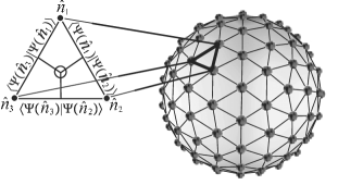
Figure 1: The vertex skeleton employed. At each vertex the ground state energy and the Kohn-Sham wavefunction are obtained and for every triangle we may form the three overlaps needed to calculate the curvature.

The computational load of this scheme is considerable and it is therefore necessary to choose an optimal covering of calculation vertices on the unit sphere. A convenient geometry is the 4-frequency icosahedron. An $n$-frequency icosahedron is an icosahedron in which each of the 20 constituent triangular surfaces has been subdivided into $n^{2}$ new triangles (see for example ref. Fuller, 1981). Fig. 1 shows the 4-frequency icosahedron with its 162 vertices, at which the ground state energies the associated Kohn-Sham wavefunctions are calculated, and 320 triangles, for which the Berry curvature values are extracted.

III Results

III.1 Structural Optimization

Structural optimization of the Co_n ($n=2,...,5$), Ni₂ clusters is carried out starting from initial atomic positions determined by Castro et. Al. Castro et al. (1997), whereby the interatomic forces are minimized and the structures refined using an accurate quasi-Newton method. Initial distances for Pd₂, Rh₂ were taken from ref. Futschek et al., 2005. In accordance with the substrate-enforced geometry (as in ref. Hirjibehedin et al., 2006), the Mn atoms are frozen equidistantly at 3.6 A, with N in between. The Mn_xN${}_{y}^{\ast}$ clusters are marked with an asterisk to indicate that the positions have not been relaxed. We will also examine the effect of allowing the atoms to relax their position on the axis. For Mn₂N₃ we start relaxation from an initial state where the N atoms are in plane but off the Mn axis.

In addition we consider the equilateral Co trimer (marked Co${}_{3}^{\ast}$) and the effect of reducing the dimer distance in Pd₂ (marked Pd${}_{2}^{\ast}$). The considered structures are shown in fig. 2 where the distances are given in units of Angstrom. Table 1 shows the resulting symmetries and binding energies.

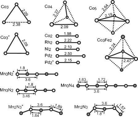
Figure 2: The considered clusters with distances in Angstrom. The asterisk indicates non-ground state configurations. In the Mn₃N${}_{4}^{*}$ cluster the atoms are equidistantly spaced at 1.8 A, like in Mn₃N${}_{2}^{*}$.

System	Symmetry	$E_{B}$ [eV]	$S$	$J$
Rh2	$C_{2h}$	3.68	2	4
Ni2	$C_{2h}$	2.87	1	1
Pd2	$C_{2h}$	1.36	1	1
Pd${}_{2}^{\ast}$	$C_{2h}$	0.69	1	2
Co2	$C_{2h}$	3.57	2	4
Co3	$C_{2h}$	6.46	$7/2$	$7/2$
Co${}_{3}^{\ast}$	$C_{3h}$	6.31	$5/2$	$3/2$
Co4	$D_{2d}$	10.01	4	4
Co5	$D_{3h}$	14.55	$13/2$	$13/2$
Co3Fe2	$D_{3h}$	14.22	$13/2$	$11/2$
Mn2N3	$C_{2h}$	14.66 (14.69)	5/2 (1/2)	5/2 (1/2)
Mn2N${}_{3}^{*}$	$C_{2h}$	12.39 (12.40)	5/2 (1/2)	5/2 (1/2)
Mn3N2	$C_{2h}$	12.83 (13.36)	13/2 (5/2)	13/2 (5/2)
Mn3N${}_{2}^{*}$	$C_{2h}$	12.67 (13.02)	15/2 (5/2)	15/2 (5/2)
Mn3N4	$C_{2h}$	20.23 (20.06)	9/2 (3/2)	9/2 (3/2)
Mn3N${}_{4}^{*}$	$C_{2h}$	19.57 (19.36)	9/2 (3/2)	9/2 (3/2)

Table 1: The symmetries, binding energies and Chern numbers of the considered clusters. The Chern numbers without ($S$) and with SOI ($J$) may differ in the presence of an SO-induced level-crossing. Values in parenthesis refer to the AFM configuration.

III.2 Chern Numbers

The Chern numbers for the considered clusters, as obtained by taking the average Berry curvature over the unit sphere, are displayed in table 1.

Figure 3: The Chern spectrum for a few selected clusters. The points show the level Chern numbers and the solid line the accumulated Chern numbers. The HOMO level and the total system Chern number have been marked with a vertical line and a circle. Deviations from $\pm\frac{1}{2}$ indicate the presence of a level-crossing as a function of increasing spin-orbit coupling strength. Multiples of half-integers have been marked with horizontal lines in order to lend support to the eye.

Fig. 3 shows the ’Chern spectrum’ for a few chosen clusters. These diagrams indicate the accumulated Chern number (the solid line), obtained by including the single-particle Kohn-Sham orbitals up to the given level in the wavefunction overlaps, and the level Chern number (the points), obtained by taking the difference between accumulated Chern number of the given level and that of its antecedent. We shall refer to the associated quantities as the level and accumulated Chern number and curvature respectively.

In Fig. 3, level Chern numbers are formed by an orbital part and a spin part obtained by taking the average curvature over the unit sphere. In the absence of SOI, the level Chern numbers can only take on values of $\pm\frac{1}{2}$. As the spin-orbit coupling strength is increased from zero, only levels that cross can deviate from this value by acquiring an orbital part. In accordance with the Chern number sum rule for level-crossings found in ref. Canali et al., 2003 - the sum of the level Chern numbers before and after the crossing is preserved. Notice that the level Chern numbers of the dimers are particularly affected by level-crossings, attributable to their inherent high degree of symmetry. Comparing the Jahn-Teller distorted Co₃ with the equilateral trimer Co${}_{3}^{\ast},$ we see that the symmetrization of the cluster leads to multiple deviations from $\pm\frac{1}{2}.$ A similar situation occurs in Co₅ when the two axial Co atoms are substituted for Fe. The level-crossing effect may in isolated cases even cause neighboring level Chern numbers to take on integer values.

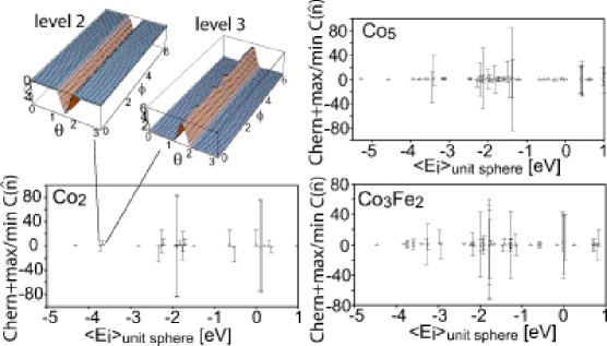
Figure 4: (Color online) The Chern number plus the maximum and minimum level curvature as a function of the average eigenenergy taken over the unit sphere. Note the large positive maximum at the HOMO-level (set to zero) of Co₂ and the induction of high-curvature variations obtained by substituting the axial Co atoms in Co₅ with Fe.

In fig. 4, we plot individual level Chern numbers together with their corresponding maximum and minimum curvature values on the unit-sphere as error bars, for a few representative clusters. Large fluctuations in the level curvature signal the presence of a near degeneracy between two adjacent levels. In general we find that a level with large fluctuations in the Berry curvature is followed by another level with curvature fluctuations of the opposite sign that nearly compensate the previous ones. (see for example the case of Co₂ where the curvature landscape of two consecutive levels is shown.) This pattern implies that although the Berry curvature of individual levels might be singular in some directions, their sum is in general a smooth function of $\hat{n}$ due to the cancellation of the opposite contributions of adjacent levels. An exception to this rule occurs when the quasi-degeneracy involves the HOMO and LUMO levels. In this case, the fluctuations of the HOMO are not compensated by the unoccupied LUMO; the total Berry curvature of the system is completely dominated by the HOMO curvature and can therefore deviate strongly from the total Chern number and be singular for particular magnetization directions. If the total curvature becomes infinite, it may be difficult to implement the procedure outlined in Sec. II.2 . In particular if the HOMO level has a predominantly minority-spin character, the total curvature can even become negative along these degeneracy directions, and the transformations given in Eqs. 10, 11 is invalid. Physically this means that when HOMO-LUMO gap goes to zero the low-energy quantum dynamics of the system cannot be described by an effective giant-spin Hamiltonian only. In this case it necessary to include explicitly all the electronic degrees of freedom involved in the degeneracy at the Fermi level. We will address this issue in more detail in Sec. IV. Depending on the given situation, one might still to a good approximation evaluate the topological effect when there are only isolated negative dips in the curvature.

System	$E_{MA}/atom$ [meV]	Type
Rh2	26	EA
Ni2	3.8	EP
Pd2	1.2	EP
Pd${}_{2}^{\ast}$	17	EA
Co2	14	EA
Co3	1.3/0.7	EA
Co${}_{3}^{\ast}$	0.8	EA
Co4	0.9	EA
Co5	0.1	EA
Co3Fe2	0.5	EA
Mn2N3	0.9/0.4 (0.8/0.4)	EA(EA)
Mn2N${}_{3}^{*}$	0.8/0.2 (0.7/0.1)	EA(EA)
Mn3N2	1.4 (0.8)	EP(EP)
Mn3N${}_{2}^{\ast}$	1.2 (1.0)	EP(EA)
Mn3N4	0.8 (1.2)	EP(EP)
Mn3N${}_{4}^{\ast}$	0.8 (0.3)	EP(EA)

Table 2: The magnetic anisotropy energies per atom. EA signifies an easy axis in parallel to the symmetry axis of the cluster, meaning the axis perpendicular to the atomic plane for Co${}_{3}^{\ast}$, the pyramid axis for Co₅ and Co₃Fe₂, the axis running through the mid-point of the two opposite solid lines in fig. 2 for Co₄. EP signifies a quasi-easy plane perpendicular to the symmetry axis running through the dimers (or the line connecting the Mn atoms). Co₃ has a high and a low barrier separating the global minima that occur when the magnetization is parallel to the elongated side. The low barrier runs in a cross-section perpendicular to the trimer plane, whereas the high barrier is in a cross-section in the trimer plane. In Mn₂N₃ the global minima are perpendicular to the cluster plane. A high barrier is separating the oppositely oriented states in a plane parallel to the Mn-Mn axis, and a low barrier separates the minima in a plane perpendicular to the Mn-Mn axis. For the Mn_xN_y clusters, the anisotropy is per Mn atom. Values in parenthesis refer to the AFM configuration.

In table 1, we see that there can be a change in the the Chern number, namely the dimensionality of the total spin system when SOI is turned on. In general this happens when the HOMO-LUMO gap is zero in the absence of the SOI. When SOI is turned on, the degeneracy is lifted but in a few nearly avoided level-crossings for particular directions of the magnetization. Berry phase contributions coming from paths encircling these quasi-degeneracies are responsible for the change in the Chern number. Thus the assumption that the dimension of effective spin the does not change when SOI is turned on is potentially a hazardous one in the case of small TM clusters.

III.3 Magnetic anisotropy energies

Let us first take a look at the magnetic anisotropy energies, before performing the variable transformation that takes us to constant curvature space. A qualitative description of the magnetic anisotropy landscapes and the associated anisotropy energies per atom, $|E_{max}(\hat{n})-E_{min}(\hat{n})|/N_{atoms}$, are presented in table 2.

To evaluate the topological effect, we first emulate a simplified approach to construct a quantized Hamiltonian by omitting the variable transformation that takes us to constant curvature space. We then take the dimension of the effective spin-system to be that inferred by the magnetic moment in the absence of SOI (i.e. the Chern number without SOI in table 1), with the assumption that turning it on causes no level-crossing. The magnetic anisotropy energy is taken to be that which we obtain by actually switching on the SOI, but should in this context be regarded as originating in a perturbational approach. Fitting the anisotropy energy with spherical harmonics limited by the system dimensionality without SOI, results in the effective quantum Hamiltonians displayed in table 3.

System	Hamiltonian	Coefficients [meV]
Rh2	$\alpha[1+\beta S_{z}^{2}+\gamma S_{z}^{4}$]S=2	$\begin{array}[c]{l}\alpha=85.1,\beta=-0.630\\ \gamma=0.095\end{array}$
Ni2	$\alpha[1+\beta S_{z}^{2}$]S=1	$\begin{array}[c]{l}\alpha=-7.68,\beta=-2.0\end{array}$
Pd2	$\alpha[1+\beta S_{z}^{2}$]S=1	$\begin{array}[c]{l}\alpha=-2.44,\beta=-2.0\end{array}$
Pd${}_{2}^{\ast}$	$\alpha[1+\beta S_{z}^{2}$]S=1	$\begin{array}[c]{l}\alpha=66.92,\beta=-1.0\end{array}$
Co2	$\ \ \alpha[1+\beta S_{z}^{2}+\gamma S_{z}^{4}]_{S=2}\ \$	$\begin{array}[c]{l}\alpha=45.3,\beta=-0.555\\ \gamma=0.076\end{array}$
$\text{Co}_{3}$	$\begin{array}[c]{c}\alpha[1+\beta S_{z}^{2}+\\ \gamma(S_{x}^{2}-S_{y}^{2})]_{S=7/2}\end{array}$	$\begin{array}[c]{l}\alpha=0.491,\beta=0.554\\ \gamma=0.10\end{array}$
Co${}_{3}^{\ast}$	$\alpha[1+\beta S_{z}^{2}$]S=5/2	$\begin{array}[c]{l}\alpha=2.88,\beta=-0.16\end{array}$
Co4	$\alpha[1+\beta S_{z}^{2}$]S=4	$\begin{array}[c]{l}\alpha=3.94,\beta=-0.063\end{array}$
Co5	$\alpha[1+\beta S_{z}^{2}$]S=13/2	$\begin{array}[c]{l}\alpha=0.589,\beta=-0.024\end{array}$
Co3Fe2	$\alpha[1+\beta S_{z}^{2}$]S=13/2	$\begin{array}[c]{l}\alpha=2.71,\beta=-0.024\end{array}$
Mn2N3	$\begin{array}[c]{c}\alpha[1+\beta S_{z}^{2}+\\ \gamma(S_{x}^{2}-S_{y}^{2})]_{S=5/2(1/2)}\end{array}$	$\begin{array}[c]{l}\alpha=0.0256(0.73)\\ \beta=10.8(0)\\ \gamma=-2.91(0)\end{array}$
Mn2N${}_{3}^{\ast}$	$\begin{array}[c]{c}\alpha[1+\beta S_{z}^{2}+\\ \gamma(S_{x}^{2}-S_{y}^{2})]_{S=5/2(1/2)}\end{array}$	$\begin{array}[c]{l}\alpha=-0.157(0.50)\\ \beta=-1.71(0)\\ \gamma=0.23(0)\end{array}$
Mn3N2	$\alpha[1+\beta S_{z}^{2}$]S=13/2(5/2)	$\begin{array}[c]{l}\alpha=-0.358(-0.619)\\ \beta=-0.308(-0.800)\end{array}$
Mn3N${}_{2}^{\ast}$	$\alpha[1+\beta S_{z}^{2}$]S=15/2(5/2)	$\begin{array}[c]{l}\alpha=-0.257(3.82)\\ \beta=-0.267(-0.160)\end{array}$
Mn3N4	$\alpha[1+\beta S_{z}^{2}$]S=9/2(3/2)	$\begin{array}[c]{l}\alpha=-0.303(-1.82)\\ \beta=-0.444(-1.33)\end{array}$
Mn3N${}_{4}^{\ast}$	$\alpha[1+\beta S_{z}^{2}$]S=9/2(3/2)	$\begin{array}[c]{l}\alpha=-0.300(1.28)\\ \beta=-0.444(-0.444)\end{array}$

Table 3: The Hamiltonians obtained by quantizing in the spin Hilbert space of the dimension given by the Chern Number without SOI (see table 1). These Hamiltonians are calculated without performing the variable transformation to constant curvature space, thereby neglecting the topological effect. This approach is designed to emulate the results one would obtain by adding the spin-orbit shifts perturbationally. The quantization axis of the big spin is taken to be the cluster symmetry axis as defined in table 2.

Generally, we find only coefficients up to second order and in isolated cases (Co₂, Rh₂) a small fourth order contribution in the spin operators. The higher order contribution is an indication of level-crossings and that non-trivial topological effects are present when SOI is switched on. If the dimension of the Hilbert space does not change when SOI is turned on, there is most likely no level-crossing at the HOMO. With a large HOMO-LUMO gap, the curvature is essentially constant with very small variations around the Chern number and there is no topological effect that enters through the variable transform (equations 10 and 11). In this case our effective Hamiltonian approach will yield the same result as in table 3.

System	$\begin{array}[c]{c}\text{\emph{Transformed}}\\ \emph{Hamiltonian}\end{array}$	Coefficients [meV]
Rh2	$\begin{array}[c]{c}\alpha[1+\beta S_{z}^{2}+\gamma S_{z}^{4}\\ +\delta S_{z}^{6}+\varepsilon S_{z}^{8}]_{J=4}\end{array}$	$\begin{array}[c]{l}\alpha=298.79,\beta=-2.3602\\ \gamma=0.94995,\delta=-0.11266\\ \varepsilon=0.0038916\end{array}$
Pd${}_{2}^{\ast}$	$\begin{array}[c]{c}\alpha[1+\beta S_{z}^{2}\\ +\gamma S_{z}^{4}]_{J=2}\end{array}$	$\begin{array}[c]{l}\alpha=6.19,\beta=12.2\\ \gamma=-3.11\end{array}$
Co2	$\begin{array}[c]{c}\alpha[1+\beta S_{z}^{2}+\gamma S_{z}^{4}\\ +\delta S_{z}^{6}+\varepsilon S_{z}^{8}]_{J=4}\end{array}$	$\begin{array}[c]{l}\alpha=145.30,\beta=-2.3058\\ \gamma=0.93035,\delta=-0.11038\\ \varepsilon=0.0038124\end{array}$
Co${}_{3}^{\ast}$	$\alpha[1+\beta S_{z}^{2}]_{J=3/2}$	$\begin{array}[c]{c}\alpha=3.03,\beta=-0.445\end{array}$
Co3Fe2	$\begin{array}[c]{c}\alpha[1+\beta S_{z}^{2}\\ +\gamma S_{z}^{4}]_{J=11/2}\end{array}$	$\begin{array}[c]{l}\alpha=2.61,\beta=-0.0235\\ \gamma=-0.000317\end{array}$
Mn2N3	$\alpha[S^{2}]_{J=1/2}^{AFM}$	$\begin{array}[c]{l}\alpha=0.137\end{array}$
Mn2N${}_{3}^{\ast}$	$\alpha[S^{2}]_{J=1/2}^{AFM}$	$\begin{array}[c]{l}\alpha=0.163\end{array}$
Mn3N${}_{2}^{*}$	$\begin{array}[c]{c}\alpha[1+\beta S_{z}^{2}\\ +\gamma S_{z}^{4}]_{J=5/2}^{AFM}\end{array}$	$\begin{array}[c]{l}\alpha=2.76,\beta=0.365\\ \gamma=-0.0840\end{array}$
Mn3N${}_{4}^{*}$	$\begin{array}[c]{c}\alpha[1+\beta S_{z}^{2}]_{J=3/2}^{AFM}\end{array}$	$\begin{array}[c]{l}\alpha=1.71,\beta=-0.444\end{array}$

Table 4: The Hamiltonians obtained by quantizing after performing the variable transformation to constant curvature space. The cases in table 3 where the transformation exhibited a very weak and negligible topological effect have been omitted above. Only the AFM Mn_xN_y have non-trivial curvatures.

III.4 Effective Chern-number spin Hamiltonians

We now consider the effect on the magnetic anisotropy obtained in performing the variable transformation to constant curvature space. Fig. 5 shows the total system curvature landscapes on the unit sphere for a few clusters, as well as the inverse of the HOMO-LUMO gap squared. This figure demonstrates that the quasi-singular behavior of the Berry curvature landscape is governed by the gap, as expected from the perturbational expression Eq. (6).

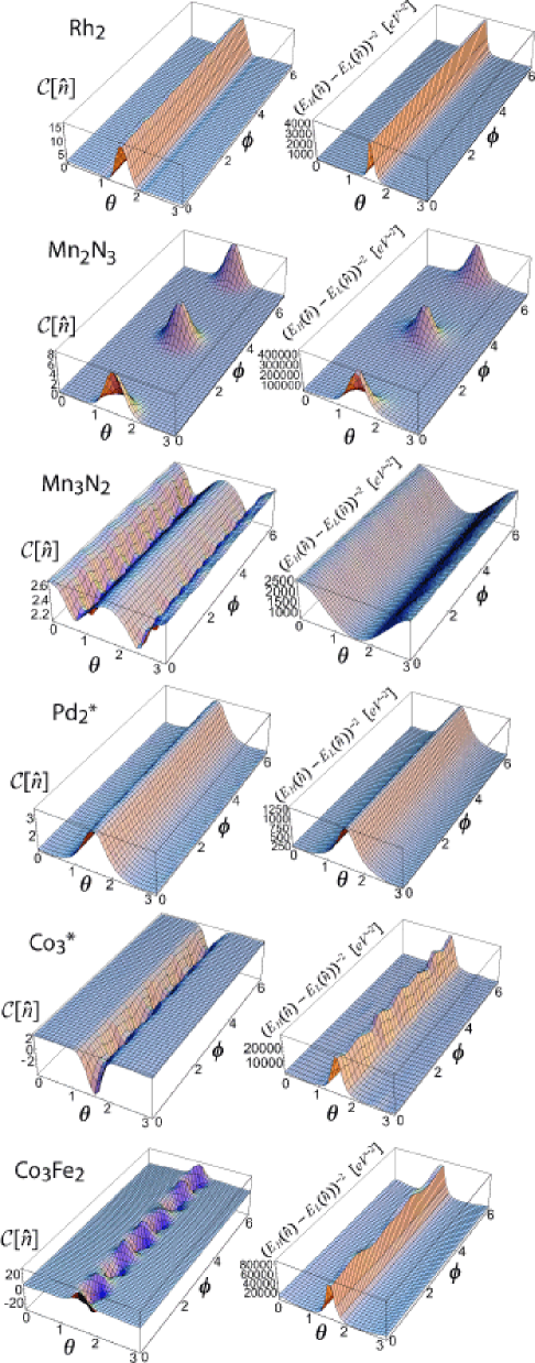
Figure 5: (Color online) The Berry curvature and the inverse of the HOMO-LUMO gap squared on the unit sphere for selected clusters. To the right of each curvature is the inverse of the associated HOMO-LUMO gap squared, demonstrating the correspondence with the perturbational expression (6). Rh₂ and Co₂ display very similar curvatures that are constant at 2, with the exception of an equatorial quasi-singular ridge that extends up to approximately 16. The AFM Mn₂N₃ and Mn₂N${}_{3}^{\ast}$ have two Gaussian peaks perpendicular to the cluster plane, extending from 0 to around 8. The AFM Mn₃N${}_{2}^{\ast}$ sticks out as the correspondence with the HOMO-LUMO gap is not entirely obvious. The three lower clusters show the triggering of a quasi-degeneracy between the HOMO and LUMO levels, by reducing the interatomic distance in Pd${}_{2}^{\ast}$, by symmetrizing the cluster geometry Co${}_{3}^{\ast}$, and by replacing the axial Co with Fe in Co₃Fe₂.

Table 4 displays the result of quantizing the classical Hamiltonian in a spin-space of a dimension dictated by the Chern number with SOI, using the transformed magnetic anisotropy energy, thus incorporating the topological effect that enters via the Berry curvature.

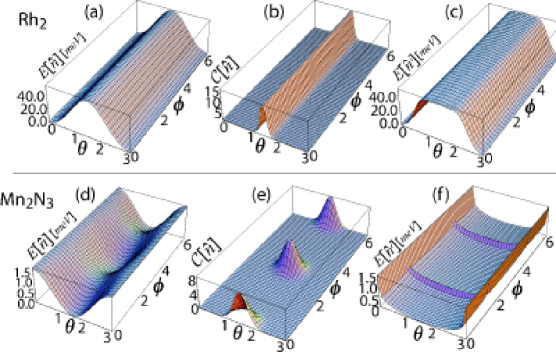
Figure 6: (Color online) The effect of the variable transform to constant curvature space for Rh₂ and Mn₂N₃. (a) and (d) show the calculated magnetic anisotropy landscape on the unit sphere and (c) and (f) show the transformed anisotropies where the topological effect of the Berry curvature (panels (b) and (e)) has been included. Rh₂ and Co₂ are topological twins and have the same curvatures and anisotropy landscapes (anisotropies differ only in magnitude due to the heavier Rh mass and stronger SOI). The equatorial quasi-singular ridge in Rh₂ and Co₂ enters the transformation and causes the effective barrier to widen significantly. The extreme Gaussian-shaped quasi-singular peaks in the curvature of Mn₂N₂ and Mn₂N${}_{2}^{\ast}$ compress the low barriers, so that the transformed anisotropy essentially becomes a shallow quasi-plane.

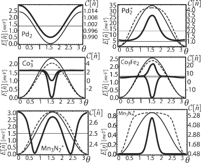
Figure 7: $\theta$-dependence of the curvature and the calculated and transformed magnetic anisotropy landscapes for selected clusters. The thick solid line is the curvature, the thin solid line the untransformed anisotropy energy and the dashed line the anisotropy energy after the variable transformation to constant curvature space has been performed. The horizontal solid lines indicate the Chern number without SOI, and the dashed ones with SOI. Pd and Ni have the same valence configuration and (although with different HOMOs) are topological twins.

Fig. 6 shows the magnetic anisotropy landscapes on the unit sphere before and after the transformation to constant curvature space for Rh₂ and Mn₂N₃, as well as the Berry curvature that enters their transform. Fig. 7 shows cross-sections of the unit sphere with transformed magnetic anisotropy energies and comparative sections with the untransformed anisotropies, as well as the Berry curvature for a few clusters. The negative dips at the equator for Co${}_{3}^{\ast}$ and Co₃Fe₂ have been cut in the transform in order to approximately capture the topological effect in these systems. Note that the transform cannot really change the magnitude of the energy values, rather, the quantization process involves the best possible fit with the allowed spherical harmonics which will average the transformed anisotropy energy into the subspace whose dimension is given by the Chern number. As a result of this averaging procedure the maximal energy is affected in accordance with the effect of the transform entering through the curvature. In the case of Co${}_{3}^{\ast}$ and Co₃Fe₂ the pull of the sub-Chern curvature on the equator is the prevailing effect, yielding a lower effective maximum. Not very surprisingly, there is no topological effect present when the HOMO-LUMO gap grows as in the case of Pd₂, Ni₂, Co_3,4,5 and the relaxed linear Mn_xN_y (these have therefore been omitted from table 4). We will now address each group of systems and the mechanisms present in detail.

III.5 Dimers

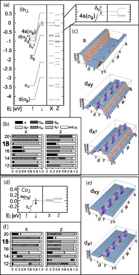
Figure 8: (Color online) Kohn-Sham orbital energies and projections of orbital character for Rh₂ and Co₂. The left panel in (a) and (d) shows the majority and minority-spin levels in the absence of SOI and the right panel the levels in the hard (x) and easy (z) direction with SOI. The origin of the large anisotropy in Rh₂ and Co₂ is a first order contribution in the spin-orbit perturbation series, resulting from the the splitting of the singly occupied but doubly degenerate HOMO-LUMO $\delta_{u}^{\ast}$-level. The HOMO (number 18) is connected with a dotted line and its population is marked with a minority spin arrow. When the SOI is turned on, the quasi-degeneracies in the hard direction split as we change the magnetization direction to the easy (symmetry) axis. Panels (b) and (f) show the orbital mixing character as given by the atomic site projected spherical harmonics taken over the spinors in the indicated direction of magnetization. Panels (c) and (e) show the orbital mixture landscapes of the HOMO on the unit sphere. The orbital mix of the HOMO (18) and LUMO (19) show that along the easy axis these states have good $m_{\ell}$ quantum numbers $\pm 2$, allowing for a continuous electron path in a plane perpendicular to the magnetization direction and a total lowering of the energy.

Transition-metal dimers have an inherent symmetry that gives them remarkable magnetic properties - they are rotationally invariant around the dimer axis. This can cause magnetic anisotropy in transition-metal dimers to appear already at first order in a perturbational treatment of the SOIStrandberg et al. (2007). Depending on the electronic configuration and the situation at the HOMO, this symmetry property can cause the magnetic anisotropy to be anomalously strong.

We will discuss the dimers in terms of their Kohn-Sham orbital energies labeled using standard molecular notationHerzberg (1950). Fig. 8 (a) and (d) show these for Rh₂ and Co₂ (around HOMO only) without SOI for majority $(\uparrow)$ and minority-spin $(\downarrow)$, and with SOI and in the hard (x) and easy (z) direction. The $s$ and $d$ valence orbitals on one atom hybridizes with orbitals on the other atom that have the same azimuthal angular momentum $m_{\ell}$, to form bonding and antibonding combinations. In the absence of SOI, these are doubly degenerate and are labeled according to their azimuthal angular momentum, where $\sigma$ refers to $m_{\ell}=0$, $\pi$ to $m_{\ell}=\pm 1$ and $\delta$ to $m_{\ell}=\pm 2$. A ^∗ indicates an antibonding orbital and u/g labels odd/even states. The SDFT exchange potential lowers majority-spin orbital energies relative to those of minority-spin type.

Both Rh₂ and Co₂ have very large magnetic anisotropies of 26 and 14 meV per atom respectively. They both exhibit an extreme topological effect due to the presence of a quasi-degeneracy at the HOMO level. The curvature (see fig. 6) is constant at 2 (note that the Chern number is 2 in the absence of SOI) all over the unit sphere, except at the equator where a quasi-singular ridge extends up to approximately 16. Fig. 8 (b) and (f) show the orbital mixing character as given by the site projected spherical harmonics inside non-overlapping atomic spheres taken over the spinors in the direction of the magnetization, for the topmost eigenlevels in the hard and easy direction (as the spheres do not overlap, some interatomic charge will be missed by the projection spheres). Using the calculated Chern spectrum (see fig. 3) in combination with the atomic site-projected orbital character for each quasi-particle level, we can extract the orbital and spin contribution parts to the level Chern number. The crucial level in both Rh₂ and Co₂ is the HOMO $\delta_{u}^{\ast}$, which is doubly degenerate but singly occupied in the absence of SOI. From the Chern spectrum of Co₂ (fig. 3) and the orbital mixing (fig. 8) we see that the HOMO (level 18) has a level Chern number of 3/2 with an orbital and spin contribution of 2 and -1/2 respectively. The orbital angular momentum is opposing the magnetization and this level will therefore be shifted down, whereas the LUMO-level with orbital part -2 and spin part -1/2 will be shifted up. The shifts in the sub-levels will to a large extent cancel each other out, but the HOMO shift remains uncompensated, causing a very large anisotropy energy. In Rh₂ the spin-orbit shift is so strong that the $\delta_{u}^{\ast}$ descends below the minority-spin 4s($\sigma_{g}$), which is much higher in energy for Rh₂ than for Co₂ - consistent with the larger dimer separation.

Up to double-counting corrections, the total energy is simply the sum of the spin-orientation-dependent shifts in occupied orbital energiesCehovin et al. (2002). In the hard direction spin-orbit shifts are small compared with the scale of the $d$-electron spin-orbit interaction ($H_{SO}=\xi_{d}\vec{s}\cdot\vec{L}$, with $\xi_{d}^{Co}\sim 85$ meV and $\xi_{d}^{Rh}\sim 140$ meV). With the spins polarized in the hard (x) direction the expectation value of $L_{x}$ over the unperturbed states is zero, and any shifts originate in higher order perturbation terms (at most $\xi_{d}^{2}/W_{d}\sim 0.1\xi_{d}$, where $W_{d}$ is the typical $d$-orbital bonding energy). However, when the spins are polarized along the easy (z) direction, i.e. the dimer axis, the first order contribution is non-vanishing and is given by $\pm\xi_{d}\langle L_{z}\rangle=\pm m_{\ell}\xi_{d}/2$. For Rh₂ and Co₂ the first order contribution is larger than the obtained anisotropy energy and the expected $|\cos(\theta)|$ appearance is not observed. This is because the cusp at the degeneracy point ($\theta=\pi/2$) is always rounded out by higher order terms, and the anisotropy energy is an even analytic function of $\cos(\theta)$. The degree of rounding is a complex many-body issue, which in our DFT calculations is affected by the smearing of occupation numbers at the HOMO. To go beyond our calculations, one would have to employ a true many-body framework, where the absence of the otherwise necessary smearing parameter would imply even larger anisotropies.

From fig. 8 it is clear that the total Chern number of 4 originates in equal parts from spin and orbital angular momentum. Without SOI there is no angular momentum contribution and in this case the total Chern number is 2 coming from the spins in the $d$-shells. With SOI the quasi-degeneracy is lifted along the easy (symmetry) axis and the total energy is lowered via the mixing of $d_{xy}$ and $d_{x^{2}-y^{2}}$ into axial eigenstates with $m_{\ell}=\pm 2$ maximal splitting and a continuous electron path in a plane perpendicular to the easy axis magnetization direction. At the equator, the $\delta_{u}^{\ast}$ levels approach each other and the curvature becomes quasi-singular. Here the $d_{xy}$ and $d_{x^{2}-y^{2}}$ characters separate and we find that the HOMO in the $x$-direction ($\phi=0$) is of pure $d_{x^{2}-y^{2}}$ character (see fig. 8 (c) and (e)).

The effect of the equatorial curvature ridge in our variable transformation of the effective big-spin Hamiltonian, is to alter the local metric (12) and repel grid-points from the equator in order to increase the subtended curvature areas in this region. This leads to a transformed magnetic anisotropy landscape that has a much wider barrier (see fig. 6). Such an enormous increase in effective barrier width should definitely lead to experimentally observable effects in terms of spin-lifetimes and tunneling probability.

The Chern number is 4, which tells us that we may use spherical harmonics of up to order $L=8$ in our quantization process. It is interesting to note that we actually need all of these to accurately describe the transformed magnetic anisotropy landscape. Omitting the smallest 8:th order coefficient leads to the formation of a non-physical shallow local minimum along the equator.

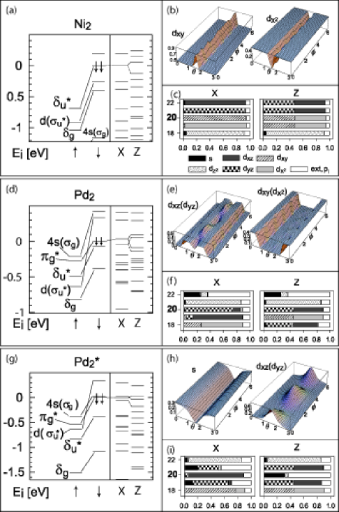
Figure 9: (Color online) Eigenlevel structure around the HOMO and atomic site projected orbital character. for the easy (x for Ni₂ and Pd₂, z for Pd${}_{2}^{\ast}$) and the hard (z for Ni₂ and Pd₂, x for Pd${}_{2}^{\ast}$) direction, as well as over the unit sphere for the HOMO. The orbitals in parenthesis are the same as the ones displayed, only with an equatorial $\phi$-dependence that is in relative anti-phase.

Paralleling the close relationship between Co and Rh, Pd and Ni have similar valence electron configurations - the 4d elements behave like their 3d counterparts. In the absence of SOI, both Co₂ and Rh₂ have a molecular groundstate $\Delta(S=2)_{g}$ and a Chern number $J=4$ with SOI. Pd₂ and Ni₂ both have a Chern number of 1 (with and without SOI) with a $\Sigma(S=1)_{g}$ ground state. Their anisotropy landscapes are quasi-easy planes perpendicular to the dimer line, although the anisotropy energies are small - balancing rather delicately between easy axis and easy plane. The curvature is essentially constant and equal to the Chern number, wherefore no topological effect enters via the variable transform (see fig. 7). The combined $s$-shell in the dimer, demotes two atomic $s$-electrons to the $d$-shell, leaving only two $d$-holes in the dimer. The net $d$-spin contribution yields the Chern number 1, with no orbital contribution. Pd₂ has a much larger dimer separation than Ni₂, which results in a different ordering of the levels. Fig. 9 (d) reveals that the $\pi_{g}^{\ast}$-level is lower in energy than the $4s(\sigma_{g})$ in Pd₂, resulting in a $\pi_{g}^{\ast}$ HOMO, whereas Ni₂ retains the $\delta_{u}^{\ast}$ (fig. 9 (a)). In both cases, the doubly degenerate HOMOs are doubly occupied. The antipodal shifts now cancel out just like for most of the sub-levels. This highlights the situation for which high anisotropy and strong topological effects are present: when there is a doubly degenerate and singly occupied HOMO in the absence of SOI. The quasi-degenerate occupied levels in Pd₂ and Ni₂ both have a highly singular level curvature, but these also cancel out, resulting in a trivial total curvature with very small variations around the Chern number. It is clear that the case of a singly occupied, doubly degenerate HOMO is the most natural candidate for a system in which there is a powerful topological effect. However, Pd${}_{2}^{\ast}$ points to another possibility. In reducing the dimer distance - the $s$-level drops in energy, until it actually intersects the HOMO-LUMO gap. In doing so, the strong topological effect (see fig. 5) is triggered due to the mixing with the $\pi_{g}^{\ast}$ doublet (see fig. 9 (g)). The non-trivial curvature enters the transform and causes the effective barrier for Pd${}_{2}^{\ast}$ to widen and the effective Hamiltonian acquires a fourth order contribution (see table 4). Note the inverse relation between the $s$-character of the HOMO (fig. 9 (h)) and the curvature (fig. 5), i.e. the curvature barrier grows as the $s$-character diminishes and the $d_{xz}(d_{yz})$-character increases.

The situation observed in Pd${}_{2}^{\ast}$, where an accidental degeneracy triggers a topological effect, by intermixing with the HOMO-LUMO doublet, can also occur in relaxed systems. For example, in C₂ Pederson and Jackson (1991), there is the exact same mechanism as in Pd${}_{2}^{\ast}$ present at the HOMO, where an $s$-level causes an accidental degeneracy with a $\pi$ HOMO, for a wide range of dimer distances.

III.6 Co₃ and Co${}_{3}^{\ast}$

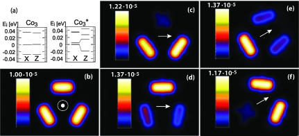
Figure 10: (Color online) Voxel projections of the Co${}_{3}^{\ast}$ HOMO and LUMO charge densities for different directions of the magnetization. (a) shows the energies of the HOMO and the LUMO for the isosceles and the equilateral trimer in the hard and easy direction. (b) shows the HOMO charge density for the equilateral trimer in a top view using maximal intensity projection. Here, a small amount of $d$-charge forms axial states and the HOMO-LUMO splitting is maximal, lowering the total energy. (c) and (e) show the HOMO charge density when the magnetization is in the hard plane along the equator. Here, the $d$-character separates, occupying the same sites as the $p$-orbitals. (d) and (f) show the corresponding LUMO charge densities which occupy increasingly disjoint regions of the cluster as the gap closes in.

Just like the symmetrized Co_4,5, the equilateral trimer Co₃ has a highly degenerate level structure and are therefore unstable against Jahn-Teller distortions (see fig. 2). Fig. 10 (a) shows the levels in close vicinity of the HOMO in the hard (x) and easy (z) direction for Co${}_{3}^{\ast}$ and the corresponding directions for the Jahn-Teller-distorted Co₃, where the hard and easy direction is interchanged relative the equilateral structure.

For the Co₃ the orbital mixing changes very little between the two directions and there is a large HOMO-LUMO gap of 0.03-0.04 eV. By contrast, the Co${}_{3}^{\ast}$ has a quasi-degeneracy in the hard direction of approximately 4 meV that is lifted to around 35 meV in the easy direction. The quasi-degeneracy that is lifted by the Jahn-Teller distortion, induces large variations from the Chern number in the curvature (see fig. 5 and 7). In fig. 3 we see that the level Chern number for the HOMO is -3/2, meaning that the HOMO level curvature that goes quasi-singular has negative curvature. Although this negative curvature is shifted by the accumulated Chern number coming from the occupied sub-levels (level 26 has an accumulated Chern number of 3 in fig. 3), negative curvature residues remain, implying that we can only approximately describe the topological impact by omitting the negative dips in the transform.

Fig. 10 shows voxel projections of the HOMO and LUMO charge densities for different directions of the magnetization. When the magnetization is in the easy (z) direction, perpendicular to the trimer plane, each atom forms a different combination of on-site $d$- and $p$-character, symmetrically around the z-axis (see fig. 10 (b)). Here, a small mixture of approximately 10% $d_{xy}$ and $d_{x^{2}-y^{2}}$ in the whole system is responsible for the lowering of the HOMO energy. On the equator (see fig. 10) (b)-(f)), these separate, different atoms are occupied by the HOMO charge and the HOMO-LUMO become quasi-degenerate. The splitting increases slightly along the equator as the magnetization changes to $\phi=\frac{\pi}{6}$ (see fig. 10 (e)), enough to produce the observed oscillations in the curvature. In the hard direction, the LUMO density occupies increasingly disjoint regions of the cluster, as the HOMO-LUMO gap closes in. The occupied configuration where the atoms are unequally occupied is higher in energy than the symmetric configuration in along the $z$-axis, resulting in a bistable configuration with a total magnetic anisotropy energy of 3 meV.

III.7 Co₅ and Co₃Fe₂

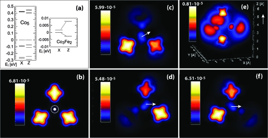
Figure 11: (Color online) The level structure around the HOMO for Co₅ and Co₃Fe₂ and voxel projections of the Co₃Fe₂ HOMO charge density for different magnetization directions. (a) shows that the substitution of the axial Co atoms in Co₅ for Fe closes the HOMO-LUMO gap from approximately 0.4 to 0.002-0.01 eV, causing an extreme quasi-degeneracy and impact on the Berry curvature. (b) shows a maximal intensity projection of the HOMO charge density when the magnetization direction is parallel to the bi-pyramidal easy-axis (top view). (c) and (d) show the HOMO densities with the magnetization in hard plane. The variations in $d$-character are responsible for the equatorial oscillations in the curvature. In (e) and (f) the LUMO charge densities when the magnetization is in the $z$- and $x$-direction are shown.

Diagrams of the level structure around the HOMO for Co₃Fe₂ and Co₅ are shown in fig. 11 (a). When the axial Co atoms in Co₅ are substituted for Fe, the character of the HOMO changes from $p$- to $d$-like. In addition, the HOMO-LUMO gap decreases from approximately 0.4 eV in Co₅ to 2-10 meV in Co₃Fe₂. This dense level structure in Co₃Fe₂ causes a level-crossing when SOI is turned on, changing the Chern number from 13/2 to 11/2. In Co₅ however, there is no level-crossing, and the Chern number does not change with the inclusion of SOI.

Fig. 2 shows that the substitutional Fe atoms compress the cluster along the bi-pyramidal axis and the center triangle increases in size. This points to the presence of an attractive force between the Fe atoms that is counteracted by the Co triangle, causing a more symmetric system with an accidental degeneracy at the HOMO. The anisotropy/atom (see table 2) increases by a factor five with the substitution - largely due to the uncompensated HOMO-downshift. Pederson et. Al Kortus et al. (2002) report a matching anisotropy/atom of 0.1 meV and moment of 13 $\mu_{B}$ for Co₅ with an increase in anisotropy/atom with a factor of approximately 5 in Co₃Fe₂. The moment of 13 $\mu_{B}$ matches our non spin-orbit Chern number, but this changes as SOI is included (see table 1). Since the large fluctuations in the curvature at the equator (see fig. 5) cancel out to a large extent in the $\theta$-variable transform (11), and since there is no $\phi$-dependence in the anisotropy landscape, the prevailing topological effect can be captured in the transform by cutting the negative dips (see fig. 7).

Fig. 11 (b)-(d) show maximal intensity projections of the HOMO charge density along the easy (z) axis and along two symmetry directions along the hard plane (the Co₃-plane). These images reveal that there is not much HOMO charge on the Fe atoms and that the dynamics of the HOMO is governed by the Co₃-triangle. In Fig. 11 (b) we see that the Co do not really form complete axial states, rather the high anisotropy comes from the fact that the states corresponding to the hard plane (Fig. 11 (c) and (d)) are relatively higher in energy. The variation of the $d$-orbitals on the different Co when the magnetization changes in the hard plane is responsible for the large equatorial oscillations. In fig. 11 (e) and (f) the LUMO charge densities are shown for a magnetization in the $z$ and $x$-direction respectively. The $z$ LUMO charge density has maximum on the Fe atoms, and is much higher in energy than the symmetric Co triangle in the HOMO.

III.8 Mn_xN_y

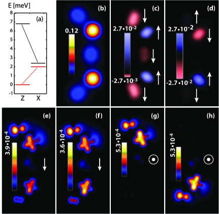
Figure 12: (Color online) Energy levels and charge densities for the HOMO and the LUMO in Mn₂N₃. (a) shows the HOMO and LUMO energies in the hard (z) and easy (x) direction. In (a), (b) and (c), the total charge density, the magnetization density in the FM variation and in the AFM variation are shown, respectively. (e) and (f) show the charge density of the HOMO and the LUMO in the $z$-direction and (g) and (h) in the $x$-direction.

Finally, we turn our attention to the hybrid Mn_xN_y clusters, partly motivated by the work of Hirjibehedin et. Al. Hirjibehedin et al. (2006). In order to properly simulate their system, it is necessary to include some layers of Cu, which, although beyond the scope of this article, certainly warrants further investigation. As the interesting topological effects occur only for the AFM configurations, we shall focus primarily on those.

We start with the Mn₂N₃-clusters. In Mn₂N${}_{3}^{\ast}$ the atoms have been locked in a configuration that corresponds to their positions as they are embedded in the covalent network of the surface. This cluster does not differ much from the Mn₂N₃, where the Mn have been frozen at a distance of 3.6 A and the N where allowed to relax starting from off Mn-axis positions. The angle of the endpoint N is some what steeper and the distance to the Mn longer because of the presence of the surface Cu atoms.

Fig. 12 (a) show how the HOMO-LUMO levels vary between the easy (x) and the hard (z) direction, for Mn₂N₃. In Mn₂N₃ the gap varies between 7 and 0.5 meV between the hard and easy direction, where as the Mn₂N${}_{3}^{\ast}$ has the same qualitative shifts but with a smaller variation from 3.5 to 1 meV. In Fig. 12 (b) the total charge density is shown, where the interspacing N atoms hold much less valence charge. (c) and (d) show the magnetization density in the Mn-axis direction, for the FM and the AFM variation respectively. The fact hat the N atoms magnetize oppositely the Mn atoms in the FM configuration, is an indication that the N stabilize the AFM configuration. The FM and the AFM configurations are rather close in energy (see table 2) although the AFM is lower in energy by the order of ten meV. As noted in by Rao et Al. Rao and Jena (2002), the presence of N in small Mn clusters, dramatically increases the binding energy and generally enhances the Mn magnetic moments, highlighting the role of the N as mediators of the AFM coupling. We find a Chern number of 1/2 in the AFM and 5/2 in the FM variation, which indicates that the N contribute to the effective cluster spin dimension. This configuration could change by the inclusion of surrounding surface Cu atoms. In the case of the dimer, a Heisenberg Hamiltonian fitted to experimental data does not lead to distinguishable results between different effective atomic Mn spins.

Fig. 12 (e) and (g) show the HOMO and (f) and (h) the LUMO charge density, in the hard (z) and easy (x) direction respectively for the Mn₂N₃ (Mn₂N${}_{3}^{\ast}$ follows a similar pattern, although less pronounced). The $p$-like charge on the N connects with the $d$-like Mn charge in one end of the cluster. The charge configurations in fig. 12 (e) and (f) results in a higher energy for the LUMO (level Chern number $-1/2$) and a lower energy for the HOMO (level Chern number $1/2$). As the magnetization is changed to the $x$-direction, the quasi-degenerate HOMO and LUMO occupy completely disjoint regions of the cluster. The energy difference between these symmetric mirror configurations is very small, resulting in severe quasi-degeneracies. These occur perpendicularly to the cluster plane and appear in the form of Gaussian shaped quasi-singularities in the curvature (see fig. 6). Their effect in the transform is to compress the low barriers to a thin line. After quantization this yields an effective quasi-plane Hamiltonian with reduced anisotropy (see tab. 4). The HOMO shift is not large enough to turn the $z$-direction into the easy direction, it does however reduce the anisotropy somewhat. In this case the MAE originates in the lower levels, whereas the its non-trivial topology is coming from the HOMO-LUMO level. The quasi-degeneracy that appears is the most severe one that we have encountered (see fig. 5). In view of this, here we expect that our single spin procedure to break down. Nevertheless, the transform gives a good indication of what is going on - the anisotropy is basically being erased by the topology of the system. The absence of spin-flip excitations in the conductance spectrumHirjibehedin et al. (2006) could very well be a manifestation of this powerful topological effect, even when the Chern number is different from zero.

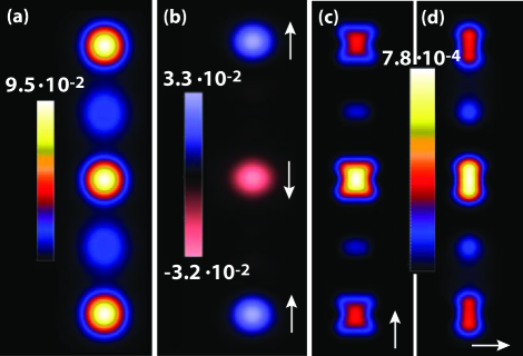
Figure 13: (Color online) Densities for Mn₃N${}_{2}^{\ast}$. (a) shows the total charge density and (b) the magnetization density in the easy (z) direction. (c) and (d) show the HOMO charge densities in the easy and hard direction, with perspective views in (e) and (g). (f) and (h) show the LUMO for the relaxed cluster which is 0.3 eV above the HOMO.

We now address the Mn₃N${}_{2}^{\ast}$. The AFM variation with Chern number 5/2 has a much lower energy than the FM variation with Chern number 15/2. This is consistent with representing the Mn with atomic spins of 5/2 and the anisotropy is of the order of what one would expect from the conduction spectrum. Mn₃N${}_{2}^{\ast}$ sticks out as there is no obvious correlation between the inverse squared of the HOMO-LUMO gap and the Berry curvature (see fig. 5). The gap size does not vary that much between hard and easy directions and is quite large, between 20-40 meV. In addition, only the HOMO moves as the magnetization direction is changed. The HOMO up-shift is in fact compensated by the sub-HOMO level, whereas the LUMO does not move at all. This is the reason for the small anisotropy the odd appearance of the curvature. Fig. 13 (a) shows the charge density and (b) the magnetization density in the easy-direction (along the cluster axis), revealing no magnetic charge on the N atoms. (c) and (d) show the HOMO charge density in the easy- and hard-direction respectively. Varying $\theta$ from 0 to $\pi$, we see that the Mn $p$- and $d$-character traces out a contour like the one observed in the curvature. The curvature causes a slight widening of the blocking barrier (see fig. 7) with a small fourth order contribution in the effective Hamiltonian (see tab. 4) When Mn₃N${}_{2}^{\ast}$ is allowed to relax into Mn₃N₂ (see fig. 2), the N position themselves relatively closer to the endpoint Mn, and the HOMO now shows no charge on the center Mn. The endpoint Mn and the N now form orbital configurations where the LUMOs are approximately 0.3 eV above the HOMO, resulting in a trivial and constant curvature. This highlights the crucial role of the epitaxial registration and the symmetry enforced by the surface. Adding two N atoms on the endpoint to create Mn₃N${}_{4}^{\ast}$ we find that the Chern numbers change to 9/2 for the FM and 3/2 for the AFM variation, consistent with instead representing the Mn with spin 3/2. Clearly the extra N alter the Mn electronic configuration, pointing to a sensitive dependence on the endpoint N positions. The FM variation yields a quasi-easy plane with a lower global minimum, and only in the AFM variation of Mn₃N${}_{4}^{\ast}$ do we find an easy axis parallel to the cluster axis. Relaxing the atoms on a line again returns the AFM to the quasi-easy plane configuration. The Mn₃N${}_{4}^{\ast}$ easy HOMO charge exhibits $p_{z}$-character on the endpoint N, but the hard direction HOMO charge has a dominant $d_{xy}$-character on the center Mn that is 17 meV higher in energy. This level is very close in energy to the hard direction LUMO, with a $d_{x^{2}-y^{2}}$-character - just a rotated version of the hard HOMO. The non-trivial Berry curvature manifests itself precisely because of this rotational symmetry. The large shift in the HOMO of 17 meV is enough to tip the scales and change the MAE from quasi-easy plane in Mn₃N₄ to an easy axis in Mn₃N${}_{4}^{\ast}$. The quasi-degeneracy in the hard plane causes a widening of the blocking barrier (see fig. 7). Quantizing with $J=3/2$ entails an averaging into the allowed spin-space, such that the widened barrier is represented by a greater effective barrier height.

IV Alternative approach at a degeneracy point

The extensive numerical studies presented above show that close to a HOMO-LUMO degeneracy we face the most interesting and difficult situation, where our giant-spin formalism is pushed to its limit: on one hand the (partly avoided) level-crossing signals that Berry curvature effects are important and large Berry curvature fluctuations modify the effective energy anisotropy lansdcape. On the other hand, when the HOMO-LUMO gap becomes too small, the ensuing singularities in the Berry curvature render the implementation of our formalism problematic, particularly when the total curvature becomes negative and the variable transformations given in Eqs. 11, 10 are not valid. In this case the description of the low-energy dynamics in terms of one single ”giant-spin” breaks down, and it is necessary to reintroduce explicitly the relevant electronic degrees of freedom responsible for the non-adiabaticity. We sketch here an alternative treatment for the spin dynamics that should remain valid when a true electronic degeneracy is present. Our idea is based on an analogy of our problem with the Jahn-Teller effect (JT) in the vibronic studies of polyatomic molecules. (For a review of the JT effect see Ref. Bersuker, 2006.) In the static JT effect, an electronic level degeneracy, usually present for a very symmetric molecular configuration, is lifted by a distortion of the molecule to a lower-symmetry configuration, accomplished via a coupling of the electronic variables with the nuclear degrees of freedom. The molecular symmetry, reduced in the static JT effect, is restored by coherent tunneling between equivalent distortions, a phenomenon known as dynamical JT (DJT) effect.

The coupled dynamics of the (fast) electronic degrees of freedom and the (slow) nuclear motion is usually investigated in two steps within the adiabatic Born-Oppenheimer (BO) approximation. Here the electronic problem is first solved for a fixed arbitrary configuration of the nuclear variables, assumed in the first instance to be classical. The resulting electronic energies act as potential energy functions for the nuclear dynamics problem, which is then treated quantum mechanical. It turns out that near an electronic degeneracy giving rise to the JT phenomena, non-adiabatic corrections to this procedure in the form of Berry phases must be taken into account. The important role of such non-adiabatic corrections was already recognized in early studies of electron-lattice interactions in molecules (see Ref. Shapere and Wilczek, 1989 for a review of this work). However, it was after Berry’s seminal workBerry (1984) that these corrections were recognized to be examples of the ubiquitous quantum geometric phases often arising in semiclassical treatments of complex quantum systems containing slow and fast degrees of freedom. The study of DJT effects in molecular systems remains a topic of great interest, which presently includes investigations of novel nanostructures carried out with the help of powerful electronic structure calculations. In this context it has recently been pointed outGarcia-Fernandez et al. (2006) that electronic structure calculations generating global minimum configurations and associated vibrational frequencies might be faulty if Berry phase effects, when present, are neglected. In general Berry phase terms affect profoundly the quantum spectrum of the vibronic dynamics.

In order to construct our analogy with the DJT effect, we first review the classical case of the JT $E\otimes e$ problem (a doubly-degenerate electronic $E$ term interacting with doubly-degenerate $e$ vibrational mode)Zwanzinger and Grant (1987); Koizumi and Bersuker (1999); Bohm et al. (2003). The Hamiltonian for the two electronic states $\{|a\rangle,|b\rangle\}$ and the doubly degenerate normal vibrational coordinates $Q_{1}=\rho\cos\theta$, $Q_{2}=\rho\sin\theta$ is $H=H_{0}+H_{1},$ where $H_{0}=\sum_{i=a,b}h_{\rm 2dho}\,|i\rangle\langle i|$, with $h_{\rm 2dho}(\rho,\theta)$ being the Hamiltonian of a two-dimensional isotropic harmonic oscillator describing the free normal modes. $H_{1}=\Big{(}k\rho e^{-i\theta}+\frac{1}{2}g\rho^{2}e^{i2\theta}\Big{)}|i\rangle\langle i|+{\rm H.c.}$ is the vibronic interaction Hamiltonian. The coordinates $Q_{1}=Q_{2}=0\leftrightarrow\rho=0$ represent the symmetric (undistorted) configuration of the molecule. The adiabatic BO potential surfaces $E_{\pm}$ are obtained by diagonalizing the electronic part of the $H$; that is, the nuclear kinetic energy is set to zero and the vibrational coordinates are treated as classical variables. For the linear $E\otimes e$ JT problem, for which $g=0$, $E_{\pm}=\frac{1}{2}\rho^{2}\pm k\rho$, and the corresponding adiabatic electronic wave functions are $|\pm(\theta)\rangle=(e^{-i\theta/2}|a\rangle\pm e^{i\theta/2}|b\rangle)\sqrt{2}$. The lowest potential energy surface has a continuous minimum at $\rho_{0}=k$, which gives rise to the JT effect. The electronic wave functions $|\pm(\theta)\rangle$ are double-valued when transported adiabatically around the degeneracy in the electronic spectrum ($E_{+}=E_{-}$) occurring at $\rho=0$. The sign change in $|\pm(\theta)\rangle$ upon encircling the origin is a manifestation of the topological Berry phase arising from the conical intersection of the adiabatic potential surface. The sign change has dramatic effect on the quantum vibration spectrum. The simplest way to see this is to consider the large $k$ regime, where the two potential surfaces are well separated. We can therefore quantize the nuclear motion by restricting to the lowest energy surface $E_{-}$. The relevant potential energy to be added to $h_{\rm 2dho}$ is therefore $V=E_{-}+H_{\rm BH}$, where $H_{\rm BH}\equiv\frac{1}{2}\sum_{i=1,2}{\partial\langle-(\theta)|\over\partial Q_{i}}{\partial|-(\theta)\rangle\over\partial Q_{i}}$ is the Born-Huang termZwanzinger and Grant (1987); Koizumi and Bersuker (1999); Bohm et al. (2003), .

Since the total vibronic wave function $\Psi(\rho,\theta)_{-}=|\rho,\theta\rangle_{-}\,\otimes|-(\theta)\rangle$ must be single-valued, the nuclear part $|\rho,\theta\rangle_{-}$ must change sign when going around the origin to compensate the double-valuedness of $|-(\theta)\rangle$. This boundary condition causes the spectrum of $h_{\rm 2dho}$ to have half-odd integral vibronic angular momentum quantum numbers. Alternatively, the sign change of $|-\rangle(\theta)$ can be absorbed by re-defining its phase. This phase change introduces a fictitious magnetic vector potential in the kinetic energy of the nuclear motion, known as Mead-Berry vector potential or Mead-Berry connection. whose curl is the Berry curvature. The presence of this fictitious magnetic field causes the same half-integer quantum numbers for the vibronic spectrum.

Quadratic and higher coupling terms in $H_{1}$ are in general important and give rise to more complex adiabatic potential energy surfaces. In particular, other conical intersections are possible, apart from the one at $\rho=0$. Typically in the $E\otimes e$ problem three other degeneracies are possible, each of them generating a Berry-Mead vector potential. In this case the overall behavior of the electronic wave functions and the resulting vibronic spectrum depend crucially on the dominant tunneling paths connecting potential energy minima, around these degeneracies: if paths encircling all four degeneracies are possible, the overall Berry phase is $4\pi$, that is, the wave functions are single-valued and the vibronic quantum numbers are integers.

In our problem with magnetic clusters, the slow nuclear motion is replaced by the collective spin degree of freedom of the cluster $\vec{S}=S\hat{n}$. This is couple to two or more electronic levels, including the HL levels, which are degenerate for given spin orientations. It is important to clarify that in this case we are not interested in the nuclear dynamics: the molecule configuration is assumed to be fixed. The Hamiltonian for the collective spin and the HL electronic levels $\{|H\rangle,|L\rangle\}$ is

$$H=H_{0}+H_{1}\;,$$ (30)

where

$$H_{0}=\sum_{i=H,L}\Big{(}{\vec{S}^{2}\over 2I}+U(\vec{S})\Big{)}|i\rangle\langle i|\;,$$ (31)

with $V(\vec{S})$ being the anisotropy energy functional without the contribution of the HL levels. Here we take $S$ to be the total spin moment of the cluster when SO coupling is switched off. The term $H_{1}$ describes the coupling between the collective spin and the HL electronic levels, and is written as

$$H_{1}=\sum_{i=H,L}V_{i}(\vec{S})|i\rangle\langle i|+\Big{(}V_{HL}(\vec{S})|H\rangle\langle L|+H.C.\Big{)}\;.$$ (32)

The functions $V_{L}$, $V_{H}$, and $V_{HL}=V_{LH}^{*}$ have to be chosen so that the eigenvalues $E_{\pm}(\vec{S})$ of $H_{1}$ reproduce the HL energy landscapes, with the associated intersections as a function of the orientation of $\vec{S}$. The eigenvalue and eigenvectors of Eq. 30 can be obtained numerically by expanding in the basis set $|\pm\vec{S}\rangle\otimes|m,S$, where $|m,S$ are eigenvectors of $S^{2}$ and $S^{z}$. However, since we want to single out the effect of the Berry phase on the slow variable dynamics, it is useful to think in terms of the adiabatic semiclassical approach and use an approximate spin Hamiltonian that includes the lowest energy surface surface $E_{-}(\vec{S})$ only. Like for the DJT problem, a conical intersection will generate a Berry phase in the electronic wavefunction, which in turn will affect the quantum spectrum of the collective spin variable $\vec{S}$. In the presence of several conical intersections, the overall effect of the Berry phase on the electronic wave function (and therefore on the dynamics of the collective spin) will depend on the character of the dominant tunneling paths connecting nearby energy minima through different saddle points around the degeneracies. As an example we can consider the case of the Co trimer. When the cluster is fixed in the static JT distorted configuration, there is no intersection between the HL energy function. Therefore the Berry phase is absent and the total spin $S$ is the same as for the case in which SO is absent. However when the trimer is fixed in a symmetric configuration, the HL gap vanishes for a few spin orientations in the plane of the clusters. Note that, as in the ordinary static JT effect, the system lifts the degeneracy by choosing a ”distorted” configuration of the slow variables (away from the ”symmetric” one) that lowers the total energy. In $Co_{3}$ this configuration is the spin orientation orthogonal to the trimer plane. An analysis of the HL energy surfaces in the trimer plane reveals that there are 6 degeneracy points separated by very shallow energy barriers. The fact that the Chern number of the cluster changes from $S=5/2$ to $S=3/2$ when SO is included, seems to indicate that paths that encircle an even number of conical intersections have dominant tunneling rates.

V Conclusions and Outlook

The crossover between macroscopic magnetic particles and atomic spins passes through the rich and complex world of magnetic nano-clusters. Interest in exploring this world is growing because of the push toward denser magnetic information storage media and an ensuing interest in achieving a deeper understanding of fundamental limits, and in identifying potentially attractive systems. From the classical point of view the most important property of a magnetic particle is the dependence of its energy on moment orientation, i.e. its magnetic anisotropy. Magnetic anisotropy in magnetic nano-clusters is due almost entirely to spin-orbit interactions which induce an orbital contribution to the moment and therefore a dependence of energy on the orientation of the moment relative to the spatial arrangement of atoms in the cluster.

In this paper our interest has been focused on the quantum effects which become important in small magnetic clusters. In particular, we have explored a SDFT-based approach to derive a giant spin low-energy effective Hamiltonian from microscopic physics. This Hamiltonian is a quantum generalization of the magnetic anisotropy energy, and describes a well-defined group of low-lying energy levels which can be identified with the magnetic moment orientation degree-of-freedom.

Our approach is orbital-based, rather than local-moment based, and is intended to enable a practical description of systems in which the spins are carried by orbitals which are widely spread over many of the cluster atoms. Loosely speaking, our approach is intended to enable a quantum description of metallic magnetic nano-clusters in which the spin-moment per atom in the absence of spin-orbit interactions is not an integer. The quantization rules of the classical anisotropy energy are calculated by adding the adiabatic Berry phase contributions from all itinerant orbitals which behave collectively in the giant spin approximation which is appropriate for slow (low-excitation energy) dynamics. We believe that the approach we have taken will be accurate whenever the fundamental assumptions which underly the giant spin approximation are valid.

In our approach both the anisotropy energy functional and the Berry curvature functional are calculated by solving the DFT Kohn-Sham equations using standard spin-polarized density functional methods that include the spin-orbit interaction. The average of the Berry curvature over magnetization directions, a topological invariant known as Berry-phase Chern number, determines the total angular momentum $J$ and reduces to the spin angular momentum $S$ in the absence of spin-orbit interactions. In our theory the Chern number determines the dimension of the quantum giant-spin Hamiltonian. We find that $J$ can deviate considerably from the total spin in the absence of spin-orbit interactions $S$ when the HOMO-LUMO gap is small. This is often the case in transition metal magnetic nano-clusters, which are often characterized by a dense level structure near the Fermi level even when the clusters are quite small. When the HL gap is small, the magnetization-dependent Berry curvature has large fluctuations and its effect on the effective spin Hamiltonian, which is usually neglected in treatments of molecular magnets, is very significant. We call this effect topological since it is related to the topological Berry-phase Chern number, and can be intuitively described as a stretching or a compression of the classical magnetic anisotropy landscape. Although we have not performed calculations for these systems, we do not expect the topological effect to be important in molecular magnets with well defined local moments. For metals however, the Berry phase effect modifies qualitatively the collective dynamics of the magnetization degree of freedom. It is clear that extremely large topological effects often signal a breakdown of the giant-spin approximation. In that case we view our approach as an attempt to construct the best possible giant-spin model.

We have carried out our DFT-based quantum giant-spin model construction procedure for dimers and for other clusters containing up to five identical atoms. We find that dimers can display a huge magnetic anisotropy because of their strong axial symmetry. For example we find anisotropies as large as $\approx 500$ K in Rh₂, which are accompanied by important topological effects that widen the magnetic anisotropy barrier between the two equivalent uniaxial minima. Both properties are closely related to the HOMO-LUMO degeneracy mentioned above, and suggest that magnetic dimer systems could be of potential technological importance for magnetic storage applications if they could be embedded in an appropriate lattice. Such large magnetic anisotropies for such small systems could represent the ultimate limit of magnetic storage capability. Furthermore thicker energy barriers will tend to increase the spin-relaxation time and suppress the microscopic quantum mechanical tunneling of the magnetization. Larger clusters such as Co₃, Co₄, and Co₅, typically manage to avoid quasi-degeneracy between the HOMO-LUMO levels by means of Jahn-Teller distortions. In this case the impact of the topological Berry curvature of the spin Hamiltonian is minor. If however a degeneracy if forced on the system by imposing a particular symmetric configuration, the singular Berry curvature once again plays a dominant role. Here we have shown that the Berry curvature can even become negative and our procedure, strictly speaking, breaks down, signaling that a description of the low-energy spectrum in terms of an individual collective spin is not possible. For these cases one is compelled to reintroduce the relevant electronic degrees of freedom involved in the degeneracy at the Fermi level. We have sketched how this procedure should be carried out in Sec. IV.

We have also looked at several hybrid clusters, in particular at linear Mn_xN_y-clusters in which the interatomic distances have been locked to mimic the effect of the epitaxial registration on a CuN surface. The study of this system is partly motivated by recent STM experimentsHirjibehedin et al. (2006) that are able for the first time to probe the collective spin dynamics of quantum engineered magnetic clusters via inelastic electron tunneling. Experimentally these clusters are found to order antiferromagnetically. We have investigated this possibility and carried out our procedure for this situation. We find that these systems show different topological effects depending on the configuration studied, and exhibit high sensitivity to the position of the N atoms coming from the CuN substrate. The results offer an alternative interpretation for the Mn dimer differential conduction spectrum and in the case of the Mn trimer our findings are compatible with the experimental results. We should however point out that our calculations are for free clusters only, namely we did not include any complicating effects originating from the supporting CuN surface that are likely to be important.

Our findings indicate that powerful effects of non-trivial spin-space topology are present in many small TM clusters, and cannot be ignored when determining the collective spin dynamics. Furthermore, our approach offers a way to extract the total spin of the system, without assigning locally defined atomic spins. Only more detailed calculations that include supporting surfaces and comparison with more accurate experiments will tell if the effects predicted by our theory can be observed in these systems.

References

- Sellmyer and Skomski (2006) D. Sellmyer and R. Skomski, eds., Advanced Magnetic Nanostructures (Springer, New York, 2006).
- Gatteschi et al. (2006) D. Gatteschi, R. Sessoli, and J. Villain, Molecular Nanomagnets (Oxford, New York, 2006).
- Sun et al. (2000) S. Sun, C. B. Murray, D. Weller, L. Folks, and A. Moser, Science 287, 1989 (2000).
- Félix-Medina et al. (2003) R. Félix-Medina, J. Dorantes-Dávila, and G. M. Pastor, Phys. Rev. B 67, 094430 (2003).
- Cehovin et al. (2002) A. Cehovin, C. M. Canali, and A. H. MacDonald, Phys. Rev. B 66, 094430 (2002).
- Skomski (2003) R. Skomski, J. Phys.: Condens. Matter 15, 841 (2003).
- Eber et al. (2005) H. Eber, S. Bornemann, J. Minar, M. Kosuth, O. Sipr, P. H. Dederichs, Zeller, and I. Cabri, Phase Transitions 78, 71 (2005).
- Kashyap et al. (2006) A. Kashyap, R. Sabirianov, and S. S. Jaswal, in Advanced Magnetic Nanostructure, edited by D. Sellmyer and R. Skomski (Springer, 2006).
- Billas et al. (1994) I. M. L. Billas, A. Châtelain, and W. A. de Heer, Science 265, 1682 (1994).
- Xu et al. (2005) X. Xu, S. Yin, R. Moro, and W. A. de Heer, Phys. Rev. Lett 95, 237209 (2005).
- Tiago et al. (2006) M. L. Tiago, Y. Zhou, M. M. G. Alemany, Y. Saad, and J. R. Chelikowsky, Phys. Rev. Lett, 97, 147201 (2006).
- Jamet et al. (2001) M. Jamet, W. Wernsdorfer, C. Thirion, D. Mailly, V. Dupuis, P. Mélinon, and A. Péres, Phys. Rev. Lett. 86, 4676 (2001).
- Gambarella et al. (2003) P. Gambarella, S. Rusponi, M. Veronese, S. S. Dhesi, C. Grazioli, A. Dallmeyer, I. Cabria, R. Zeller, P. H. Dederichs, K. Kern, et al., Science 300, 1130 (2003).
- Gambarella et al. (2002) P. Gambarella, A. Dallmeyer, K. Maiti, M. C. Malagoli, W. E. amd K. Kern, and C. Carbone, Nature 416, 301 (2002).
- Mokrousov et al. (2006) Y. Mokrousov, G. Bihlmayer, S. Heinze, and S. Blügel, Phys. Rev. Lett, 96, 147201 (2006).
- Strandberg et al. (2007) T. O. Strandberg, C. M. Canali, and A. H. MacDonald, Nature Materials 6, 648 (2007).
- Bode et al. (2004) M. Bode, O. Pietzsch, A. Kubetzka, and R. Wiesendanger, Phys. Rev. Lett, 92, 067201 (2004).
- Gunther and Barbara (1995) L. Gunther and B. Barbara, eds., Quantum Tunneling of Magnetization, QTM 94 (Kluwer, Dordrecht, 1995).
- Chudnovsky and Tejada (1998) E. Chudnovsky and J. Tejada, Macroscopic Quantum Tunneling of the Magnetic Moment (Cambridge University Press, Cambridge, 1998).
- Hirjibehedin et al. (2006) C. F. Hirjibehedin, C. P. Lutz, and A. J. Heinrich, Science 312, 1021 (2006).
- Canali et al. (2003) C. M. Canali, A. Cehovin, and A. H. MacDonald, Phys. Rev. Lett. 91, 046805 (2003).
- Berry (1984) M. V. Berry, Proc. R. Soc. A 392 (1984).
- Resta (2000) R. Resta, J. Phys.: Condens. Matter 12, 107 (2000).
- Auerbach (1994) A. Auerbach, Interacting Electron and Quantum Magnetism (Springer-Verlag, New York, 1994).
- Bohm et al. (2003) A. Bohm, A. Mostafazadeh, H. Koizumi, Q. Niu, and J. Zwanziger, The Geometric Phase in Quantum Systems (Springer-Verlag, New York, 2003).
- Cehovin et al. (2003) A. Cehovin, C. M. Canali, and A. H. MacDonald, Phys. Rev. B 68, 014423 (2003).
- Uhl et al. (1994) M. Uhl, L. M. Sandratski, and J. Kuber, Phys. Rev. B 50, 291 (1994).
- Niu and Kleinman (1998) Q. Niu and L. Kleinman, Phys. Rev. Lett. 80, 2205 (1998).
- Niu et al. (1999) Q. Niu, X. Wang, L. Kleinman, W. M. Liu, D. M. C. Nicholson, and G. M. Stocks, Phys. Rev. Lett. 83, 207 (1999).
- Gebauer and Baroni (2000) R. Gebauer and S. Baroni, Phys. Rev. B 61, 6459 (2000).
- Bylander et al. (2000) D. M. Bylander, Q. Niu, and L. Kleinman, Phys. Rev. B 61, 11875 (2000).
- Blochl (1994) P. E. Blochl, Phys. Rev. B 50, 17953 (1994).
- Kresse and Furthmuller (1996) G. Kresse and J. Furthmuller, Comput. Phys. Commun. 6 (1996).
- Kresse and Joubert (1999) G. Kresse and J. Joubert, Phys. Rev. B 59, 1758 (1999).
- Vosko et al. (1980) S. H. Vosko, L. Wilk, and M. Nusair, Can J. Phys. 58, 1200 (1980).
- Hobbs et al. (2000) D. Hobbs, G. Kresse, and J. Hafner, Phys. Rev. B 62, 11556 (2000).
- Pederson and Jackson (1991) M. R. Pederson and K. A. Jackson, Phys. Rev. B 43, 7312 (1991).
- Jamorski et al. (1997) C. Jamorski, A. Martinez, M. Castro, and D. R. Salahub, Phys. Rev. B 55, 10905 (1997).
- Micherlini et al. (1998) M. C. Micherlini, R. P. Diez, and A. H. Jubert, Int. J. of Quantum Chem. 70, 699 (1998).
- Koelling and Harmon (1977) D. D. Koelling and B. N. Harmon, J. Phys. C 10, 3107 (1977).
- MacDonald et al. (1980) A. H. MacDonald, W. E. Pickett, and D. D. Koelling, J. Phys. C 13, 2675 (1980).
- Carrier and Wei (2004) P. Carrier and S.-H. Wei, Phys. Rev. B 70, 035212 (2004).
- Fuller (1981) Fuller, Critical Path (St. Martin’s Press, New York, 1981).
- Castro et al. (1997) M. Castro, C. Jamorski, and D. R. Salahub, Chem. Phys. Lett. 271, 133 (1997).
- Futschek et al. (2005) T. Futschek, M. Marsman, and J. Hafner, J. Phys.: Condens. Matter 17, 5927 (2005).
- Herzberg (1950) G. Herzberg, Molecular Spectra and Molecular Structure (Van Nostrand Reinhold, New York, 1950).
- Kortus et al. (2002) J. Kortus, T. Baruah, and M. R. Pederson, Appl. Phys. Lett. 80, 4193 (2002).
- Rao and Jena (2002) B. K. Rao and P. Jena, Phys. Rev. Lett. 89, 185504 (2002).
- Bersuker (2006) I. Bersuker, The Jahn-Teller Effect (Cambridge University Press, Cambridge, England, 2006).
- Shapere and Wilczek (1989) A. Shapere and F. Wilczek, Geometric Phases in Physics (World Scientific, 1989).
- Garcia-Fernandez et al. (2006) P. Garcia-Fernandez, I. B. Bersuker, and J. E. Boggs, Phys. Rev. Lett. 96, 163005 (2006).
- Zwanzinger and Grant (1987) J. Zwanzinger and E. Grant, J. Chem Phys. 87, 2954 (1987).
- Koizumi and Bersuker (1999) H. Koizumi and I. B. Bersuker, Phys. Rev. Lett. 83, 3009 (1999).