The effect of ambipolar resistivity on the formation of dense cores

Abstract

Aims. We aim to understand the formation of dense cores by magnetosonic waves in regions where the thermal to magnetic pressure ratio is small. Because of the low-ionisation fraction in molecular clouds, neutral and charged particles are weakly coupled. Ambipolar diffusion then plays an important rôle in the formation process.

Methods. A quiescent, uniform plasma is perturbed by a fast-mode wave. Using 2D numerical simulations, we follow the evolution of the fast-mode wave. The simulations are done with a multifluid, adaptive mesh refinement MHD code.

Results. Initial perturbations with wavelengths that are 2 orders of magnitude larger than the dissipation length are strongly affected by the ion-neutral drift. Only in situations where there are large variations in the magnetic field corresponding to a highly turbulent gas can fast-mode waves generate dense cores. This means that, in most cores, no substructure can be produced. However, Core D of TMC-1 is an exception to this case. Due to its atypically high ionisation fraction, waves with wavelengths up to 3 orders of magnitude greater than the dissipation length can be present. Such waves are only weakly affected by ambipolar diffusion and can produce dense substructure without large wave-amplitudes. Our results also explain the observed transition from Alfvénic turbulent motion at large scales to subsonic motions at the level of dense cores.

1 Introduction

Observations show that molecular clouds are highly structured (e.g. Blitz & Stark BS85 (1986)). Furthermore, emission-line profiles of molecular tracers such as CO and CS are considerably broader than their thermal line widths indicating the presence of highly turbulent motions (e.g. Falgarone & Phillips FP90 (1990)). Since molecular clouds are threaded by magnetic fields, it is natural to suppose that these observed line widths are due to magnetohydrodynamic (MHD) waves (Arons & Max AM75 (1975)).

Large-scale, three-dimensional (3D) simulations of turbulent gas motions (e.g. Ballesteros-Paredes & Mac Low BM02 (2002); Padoan & Nordlund PN02 (2002); Gammie et al. Getal03 (2003); Li et al. Letal04 (2004); Galván-Madrid et al. Getal07 (2007)) show that dense cores with statistical properties similar to those observed can indeed be formed in this way. By following the evolution of a single MHD wave, Falle & Hartquist (FalleHartquist02 (2002)) in 1D and Van Loo et al. (VanLooetal06 (2006)) in 2D found that dense cores could be generated by the excitation of slow-mode waves. This process works on different length-scales and can also explain the formation of substructure within cores themself (Van Loo et al. VanLooetal07 (2007)).

In all these simulations, the plasma is treated as a single ideal plasma in which the plasma is perfectly coupled with the magnetic field. However, the low ionisation fraction in molecular clouds (Elmegreen E79 (1979)) implies that the plasma and magnetic field are actually weakly coupled on the scale of the cores. The charged particles then drift through the neutral particles giving rise to ambipolar diffusion (Mestel & Spitzer MS56 (1956)). Large-scale, 3D simulations including ambipolar resistivity (Padoan et al. PZN00 (2000); Oishi & Mac Low OM06 (2006)) show that dense cores still arise in those conditions. Lim et al. (Limetal05 (2005)) investigated in 1D the effect of ambipolar resistivity on the evolution of a single MHD wave. They found that ambipolar diffusion affects the evolution of waves with wavelengths up to about a thousand times the dissipation length-scale and thus has a significant effect on much of the observed structure in star formating regions.

In this paper we extend the model of Lim et al. (Limetal05 (2005)) to two dimensions. The governing equations and the initial condition are given in Sect. 2. We then examine the density structure in the numerical calculations (Sect. 3). and discuss the relevance of these results in Sect. 4.

2 The model

2.1 Governing equations

Since the ionisation fraction within molecular clouds is low, the plasma needs to be treated as a multicomponent fluid consisting of neutrals, and charged particles. Here we assume the charged particles to be ions and electrons only. In the limit of small mass densities for the charged fluids, their inertia can be neglected. The governing equations for the neutral fluid are given by

$$\frac{\partial{\rho_{n}}}{\partial{t}}+\nabla(\rho_{n}{\bf v}_{n})=0,$$ (1)

$$\frac{\partial{\rho_{n}{\bf v}_{n}}}{\partial{t}}+\nabla(\rho_{n}{\bf v}_{n}{\bf v}_{n}+p_{n})={\bf J}\times{\bf B},$$

with $\nabla=(\partial/\partial{x},\partial/\partial{y})$. For the charged fluid $j$, the equations reduce to

$$\frac{\partial{\rho_{j}}}{\partial{t}}+\nabla(\rho_{j}{\bf v}_{j})=s_{jn},$$ (2)

$$\alpha_{j}\rho_{j}({\bf E}+{\bf v}_{j}\times{\bf B})+\rho_{j}\rho_{n}K_{jn}({\bf v}_{n}-{\bf v}_{j})=0.$$

where $\alpha_{j}$ is the charge to mass ratio, $K_{jn}$ the collision coefficient of the charged fluid $j$ with the neutrals, $s_{jn}$ the mass transfer rate between the charged fluid $j$ and the neutral fluid, $\bf{B}$ the magnetic field, $\bf{E}$ the electric field and $\bf{J}$ the current given by $\bf{J}=\sum_{j}{\alpha_{j}\rho_{j}\bf{v}_{j}}$. We adopt an isothermal equation of state $p=\rho T$ for all fluids with $T$ the isothermal temperature. Note that the units are chosen so that all factors of $4\pi$ and $c$ disappear from the equations.

Within translucent clumps the ionisation fraction, $X_{i}$, changes as a function of the neutral density (e.g. Ruffle et al. Ruffleetal98 (1998)). For a visual extinction of $A_{V}=3$, the ionisation fraction decreases from $X_{i}=10^{-4}$ for $n_{H}\leq 1000\leavevmode\nobreak\ {\rm cm^{-3}}$ to $X_{i}=10^{-7}$ for $n_{H}=5\times 10^{4}$ cm^-3, roughly following a $1/n_{H}$ law. As the ionisation and recombination rates are sufficiently high in molecular clouds, ionisation equilibrium is quickly reached. We therefore adopt mass transfer rates $s_{jn}$ so that the fractional abundances of ions and electrons vary as $1/n_{H}$.

The Hall parameters of the ions and electrons, i.e. the ratio between their gyrofrequency and the collision frequency with the neutrals, are large in most astrophysical situations (Wardle Wardle98 (1998)). The ions and electrons thus gyrate many times around a magnetic field line before they collide with a neutral particle. These collisions affect the evolution of the magnetic field which is governed by

$$\frac{\partial{{\bf B}}}{\partial{t}}-\nabla\times({\bf v}_{n}\times{\bf B})=\nabla\times\left(r_{a}\frac{((\nabla\times{\bf B})\times{\bf B})\times{\bf B}}{B^{2}}\right),$$ (3)

where $r_{a}$ is the ambipolar resistivity (Falle Falle03 (2003)). As the electrons have a Hall parameter which is larger than the ions, the ambipolar resistivity is given by

$$r_{a}=\frac{B^{2}}{\rho_{i}\rho_{n}K_{in}}.$$

Equations 1 - 3 are solved with an adaptive mesh refinement code using the scheme described by Falle (Falle03 (2003)) which we extended to two dimensions. This scheme uses a second-order Godunov solver for the neutral fluid equations (Eqs. 1a and b). The charged fluid densities are calculated using an explicit upwind approximation to the mass conservation equation (Eq. 2a), while the velocities can be calculated from the reduced momentum equations (Eq. 2b). The magnetic field is advanced explicitly, even though this implies a restriction on the stable time step at high numerical resolution due to the ambipolar resistivity term, i.e. $\Delta t<\Delta x^{2}/4r_{a}$ (Falle Falle03 (2003)).

The code uses a hierarchy of grids such that the grid spacing of level n is $\Delta x/2^{n}$, where $\Delta x$ the grid spacing of the coarsest level. The solution is computed on all grids and the difference between the solutions on neighbouring levels is used to control refinement. More specifically, if the mapped down coarse cell value of the neutral flow variables differs by more than 10% from the fine cell value, the grid is refined. The loss in efficiency due to the time step restriction is then partially balanced by the gain due to adaptive mesh refinement. We also implemented the divergence cleaning algorithm of Dedner et al. (Dedneretal02 (2002)) to eliminate the errors due to non-zero $\nabla\cdot{\bf B}$.

2.2 Initial conditions

Like Lim et al. (Limetal05 (2005)) we study the formation of dense inhomogeneities by following the evolution of a fast-mode wave in a uniform plasma in which the magnetic pressure dominates over the gas pressure. Slow-mode waves are not excited in the initial state. They have a very low propagation speed, and will therefore remain localised near the boundary until they are generated inside the cloud by nonlinear steepening of the fast-mode wave.

The quiescent, uniform background plasma conditions are given (in dimensionless units) by

$$\rho_{n}=1,\rho_{e}=5\times 10^{-8},\rho_{i}=10^{-3},{\bf v}_{n,i,e}=0,B_{x}=1,B_{y}=0.25,$$

and an isothermal temperature $T=0.015$ for all fluids. Furthermore, we adopt $\alpha_{e}=-2.0\times 10^{12}$ and $\alpha_{i}=10^{8}$ for the electron and ion charge to mass ratio, and $K_{en}=4.0\times 10^{5}$ and $K_{in}=2.0\times 10^{4}$ for the electron and ion collision coefficients. These values correspond to the properties of a translucent clump with optical extinction $A_{V}=3$, a neutral number density of 500 cm^-3 and a magnetic field of 30 $\mu$G for a core temperature of 10 K. Note that we adopt $m_{n}=2m_{H}$ and $m_{i}=10m_{H}$ for the neutral and ion mass. The adopted value for the ion mass lies well within the observed range, i.e. from $\approx 3m_{H}$ when H${}^{+}_{3}$ is the dominant ion to $\approx 30m_{H}$ when it is HCO⁺ (Caselli et al. Casellietal02 (2002)).

A non-linear fast magnetosonic wave propagating in the positive $x$-direction is then superposed onto the uniform background. The initial state needs to be calculated using the method described in Lim et al. (Limetal05 (2005)) and Van Loo et al. (VanLooetal07 (2007)), since a simple linear approximation is not valid. This method requires that a wave satisfies

$$\frac{\partial{{\bf P}}}{\partial{x}}\propto{\bf r}_{f},$$

where ${\bf P}$ is the vector of the primitive variables $\rho,{\bf v}$ and ${\bf B}$, and ${\bf r}_{f}$ the right fast-mode eigenvector (see Falle & Hartquist FalleHartquist02 (2002)). By specifying the profile for $v_{y}(x,y)$, all other primitive variables can be easily calculated. We assume that, for all fluids, the $y$-component of the velocity associated with the wave changes sinusoidally with $x$. Furthermore, we introduce a sinusoidal phase-shift with respect to the $y$-direction to make the flow two-dimensional, so that

$$v_{y}(x,y)=A_{1}\sin\left[\frac{2\pi}{\lambda}\left(x+A_{2}\sin\left(\frac{2\pi y}{\lambda_{2}}\right)\right)\right],$$

where $\lambda$ is the wavelength of the fast-mode wave, $\lambda_{2}$ the wavelength of the perturbation in the $y$-direction and $A_{2}$ the amplitude of the phase shift in the $y$-direction. $A_{1}$ is the amplitude of the $y$-component of the velocity and is chosen so that the maximum amplitude of the total velocity in the wave ($\sqrt{v^{2}_{x}+v^{2}_{y}})$ is a specified value $A$. We perform calculations for $A=0.7$, 1.0 and 1.5. As the Alfvén speed, $v_{a}=B/\sqrt{\rho}$, is roughly 1.0 in our simulations, these models correspond to sub-, trans- and super-Alfvénic perturbations. As in to Van Loo et al. (VanLooetal06 (2006)), we set $A_{2}=0.01\lambda$ and $\lambda_{2}=\lambda$. The spatial variations in the fast-mode waves with different wavelength $\lambda$ are then identical and any differences in the dynamical evolution is due to the physical processes and not the initial conditions.

Due to the ambipolar resistivity in a weakly ionised plasma, a fast-mode magnetosonic wave of long wavelength $\lambda$ dissipates on a time-scale

$$t_{d}=\frac{\lambda^{2}}{r_{a}}.$$

Since we are interested in the generation of dense structures associated with slow-mode waves, it is necessary that the initial fast-mode wave can generate these slow-mode waves before it dissipates. The time for the wave to steepen into a shock is roughly

$$t_{s}=\frac{\lambda}{2A_{1}},$$ (4)

which gives the following condition

$$\lambda>>\frac{r_{a}}{2A_{1}}=\frac{0.025}{A_{1}},$$

for dissipation to be unimportant initially. Like Lim et al. (Limetal05 (2005)), we study the evolution of fast-mode waves with $\lambda=\pi$ and $10\pi$ which satisfy the above condition. The numerical domain is $0\leq x\leq\lambda$ and $0\leq y\leq\lambda$ with periodic boundary conditions. We use 4 grid levels with a finest grid resolution $800\times 800$.

We also do simulations for $\lambda=100\pi$, but these are done with the ideal MHD code described in Falle (Falle91 (1991)). This is because we cannot resolve shocks if $\lambda=100\leavevmode\nobreak\ \pi$ with the above resolution. The physical shock thickness, which is of the order of the ambipolar dissipation length $l_{d}$, is smaller than the finest grid spacing. (The dissipation length $l_{d}$ is the wavelength of the wave that dissipates in one wave period, i.e. $c_{f}t_{d}=\lambda$ with $c_{f}$ the fast-magnetosonic speed and $l_{d}=0.05$ in our simulations.) This itself is not a problem as the numerical scheme smears out the shock front over a few grid cells. However, the magnetic field then appears discontinuous on the grid and this cannot be handled by our numerical procedure (see Falle Falle03 (2003)). Although we could use higher numerical resolution this increases the computational cost considerably and is unnecessary since the results of Lim et al. (Limetal05 (2005)) show that dissipation is negligible for $\lambda\geq 30\pi$ and the flow can be treated as a single ideal fluid.

3 Results

3.1 Large wavelengths, e.g. $\lambda=100\pi$

It is useful to first consider the evolution of fast-mode waves in the absence of ambipolar dissipation. This is not only an appropriate description for waves with wavelengths larger than $\approx 30\pi$ (see above), it also allows us to properly describe the effect of ambipolar dissipation.

Van Loo et al. (VanLooetal06 (2006)) performed similar simulations in which they followed small-amplitude fast-mode waves. These simulations show that the first dense structures are formed by the non-linear steepening of the wave and that the subsequent interaction of the fast-mode shock with these dense regions generates additional structure. Since non-linear steeping occurs earlier for larger initial amplitudes (see Eq. 4), we would expect dense structures to appear earlier for such waves. Furthermore, it was shown that larger wave amplitudes result in larger density contrasts, i.e. $\rho_{\rm max}\propto A_{1}^{2}$. Figure 1 shows that this dependence still holds for finite-amplitude waves.

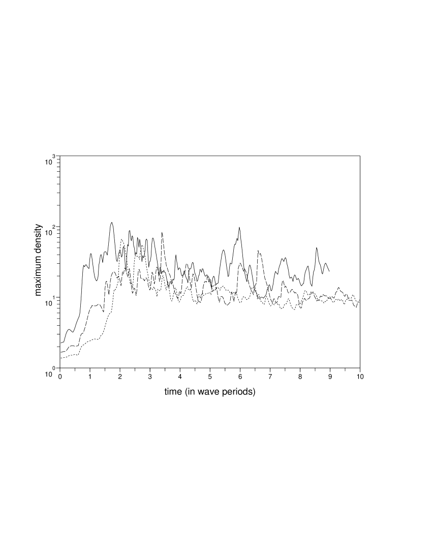
Figure 1: Temporal evolution of the maximum normalised number density for $\lambda=100\pi$ with different wave amplitudes: A = 1.5 (solid), 1.0 (dashed) and 0.7 (dotted). The normalisation factor is $n_{H}=10^{3}$ cm^-3.

The density structure for finite-amplitude waves is more filamentary than produced by the small-amplitude waves. This is a result of the more rapid steepening of the fast-mode wave and the concurrent faster growth of the perturbation in the $y$-direction. Figure 2 shows that some substructure with $\rho>10$, or $n_{H}>10^{4}$ cm^-3 ($\rho=1$ corresponds to $n_{H}=10^{3}$ cm^-3, see Sect. 2.2), is present within these filaments. As these density structures have densities higher than the threshold for line emission of NH₃, they can, in a traditional sense, be referred to as dense cores (e.g. di Francesco et al. dFetal07 (2007)). In our simulations, dense cores arise where a shock interacts with another shock or with an already present dense region. In such interactions slow-mode waves are excited which are associated with density enhancements (e.g. Falle & Hartquist FalleHartquist02 (2002); Van Loo et al. VanLooetal06 (2006)).

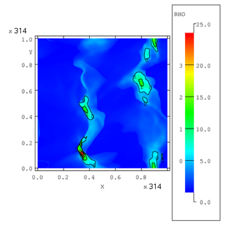
Figure 2: Density structure for $\lambda=100\pi$ with wave amplitude $A_{1}=1.5$ after 4 wave periods. The contour lines indicate normalised number densities higher than 5, 10, 15 and 20. The same normalisation factor as in Fig. 1 is used.

Although the initial fast-mode wave is not affected by ambipolar dissipation, it can be expected that the dense cores are. However, slow-mode waves associated with dense cores do not generate large perturbations in the magnetic field (see e.g. Falle & Hartquist FalleHartquist02 (2002)). (Note that this means that the magnetic field within a dense core is roughly the same as the background magnetic field.) As ambipolar diffusion only acts on the magnetic field, slow-mode waves propagate without any significant damping (Balsara Balsara96 (1996)). The lifetimes of gravitationally unbound dense cores are, therefore, not determined by the ambipolar dissipation, but by the dispersion time-scale of a core. This dispersion time scale is given by $t_{\rm disp}\approx r/v_{a}$, where $r$ is the core radius, and is generally short compared to the wave period of the initial wave. Figure 1 shows that high-density contrasts are present for several wave periods. Slow-mode excitation and the associated dense core formation only ceases when the fast-mode shock has dissipated away most of its energy. The formation of structure is therefore driven by the fast-mode wave.

3.2 Intermediate wavelengths, e.g. $\lambda=10\pi$

For the wave-amplitudes studied here, a fast-mode wave with a wavelength $\lambda=10\pi$ steepens into a shock before ambipolar diffusion becomes important. Although this suggests a similar evolution for waves with $\lambda=10\pi$ as for $\lambda=100\pi$, there are some important differences. Figure 3 shows that the high-density structures develop later than for $\lambda=100\pi$ (see Fig. 1). Also, the maximum densities within cores are roughly a factor of 5-10 smaller. Note that for $\lambda=10\leavevmode\nobreak\ \pi$, $\lambda/l_{d}=200\leavevmode\nobreak\ \pi$ and that ambipolar resistivity is thus important even for waves with wavelengths that are rather large compared to the dissipation length.

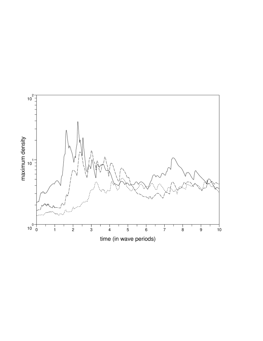
Figure 3: Same as Fig. 1 but for $\lambda=10\pi$.

It is not the fast-mode wave that is significantly affected by ambipolar diffusion, but the initial perturbation perpendicular to the propagation direction is. So far, we have neglected its rôle in the dynamics. The initial $y$-dependent contribution of the perturbation due to the phase-shift of the fast-mode wave has the same wavelength as the fast-mode wave, but the amplitude of the variations in the magnetic field due to this phase shift are about two orders of magnitude (or more) smaller. The variations in the $y$-direction will therefore dissipate more quickly than the those in the $x$-direction. Evidently, the variations perpendicular to the magnetic field grow more slowly. Figures 4 a and b show the difference in the growth of these variations for $\lambda=100\pi$ and $\lambda=10\pi$.

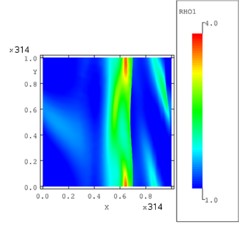
Figure 4: The normalised density structure at half a wave period for $\lambda=100\pi$ (upper panel) and $\lambda=10\pi$ (lower panel) with A=1.5. The density range is set between 1 and 4 with the same normalisation factor as in Fig. 1.

As a result, it becomes more difficult to produce large density perturbations. The largest density inhomogeneities form within dense filaments due to the interaction of these regions with shocks (e.g. Van Loo et al. VanLooetal06 (2006)). The core density thus depends on the density of the parent filament and of the shock strength. In this case, not only do the filaments have smaller densities than for $\lambda=100\pi$, but the shock strength is continuously decreasing due to the ambipolar dissipation. This also explains why there is only a short period of time (i.e. $\approx$ 3-4 wave periods) for which we find peak densities with $\rho>10$ or $n_{H}>10^{4}$ cm^-3.

3.3 Short wavelengths, e.g. $\lambda=\pi$

In the previous section, we found that ambipolar dissipation has a moderate effect on the evolution of waves with a wavelength $\lambda=10\pi$. For shorter wavelengths, i.e. $\lambda=\pi$, the impact is greater even though the wave is two orders of magnitude longer than the dissipation length. The initial $y$-dependent contribution to the perturbation is, as can be expected from the previous case, not large enough to develop any significant variation in that direction. This means that there are only variations in the $x$-direction (see Fig. 5). The evolution of the wave is then nearly one-dimensional.

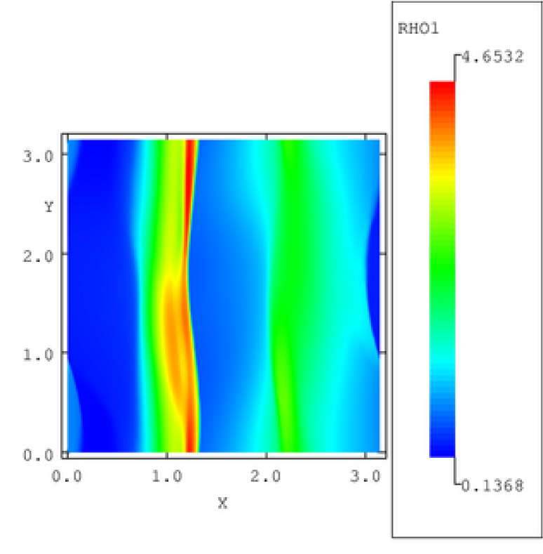
Figure 5: The normalised density structure after 3 wave periods for $\lambda=\pi$ with $A=1.5$.

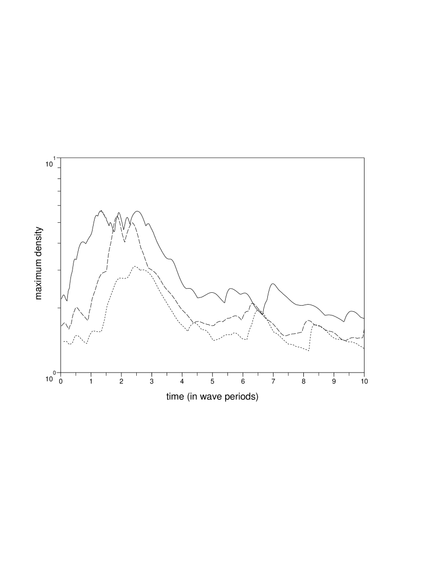
Figure 6: Same as Fig. 1 but for $\lambda=\pi$.

Ambipolar dissipation causes rapid decay of the fast-mode wave: the shock wave loses its energy within a few wave periods. The generation of density inhomogeneities then stops, as can be seen in Fig. 6. The dissipation process, however, also contributes to the formation of density structures at short wavelengths. Lim et al. (Limetal05 (2005)) showed that, for $\lambda\approx\pi$, ambipolar dissipation plays a major rôle in the excitation of slow-mode waves. Figure 6 indeed shows that the density contrasts arise earlier than for $\lambda=10\pi$. However, ambipolar diffusion is still more efficient in reducing the peak density which does not become much higher than $\rho=5$ or $n_{H}=5\times 10^{3}$ cm^-3.

To break the one dimensionality of the flow and form cores, the initial phase shift needs to be larger than in our standard model: the variations of the magnetic field in the $y$-direction should be of the same order as the $x$-direction. Additional simulations for $\lambda=\pi$ with $A_{2}>0.1\lambda$ produce dense cores with sizes of the order of the dissipation length. The maximum density is roughly 2-3 times higher than in the standard model (see Fig. 6) even for the largest wave amplitudes. This means that fast-mode waves with wavelengths that are 2 orders of magnitude longer than the dissipation length can only form cores in a highly turbulent plasma.

4 Discussion and conclusions

In this paper we studied the formation of density structures in a weakly ionised plasma by following the evolution of a fast-mode wave. This adequately describes the formation of dense cores in a clump which is perturbed at its edge. Slow-mode waves propagate at low speeds and remain near the boundary. Fast-mode waves propagate much faster and produce slow-mode waves within a clump either due to non-linear steepening or interactions with denser regions. However, in a weakly ionised plasma, the ion-neutral drift is an important dissipation process. We find that ambipolar resistivity strongly affects the evolution of fast-mode waves with wavelengths up to 2 orders of magnitude larger than the dissipation length.

For an MHD wave in which the velocities are of the order of the Alfvén speed, the ambipolar dissipation length-scale is given by (e.g. Osterbrock O61 (1961); Kulsrud & Pearce KP69 (1969))

$$l_{d}=100\left(\frac{B}{30\mu G}\right)\left(\frac{10^{-4}}{X_{i}}\right)\left(\frac{1000}{n_{H}}\right)^{3/2}{\rm AU},$$ (5)

so that $\lambda=\pi\approx$ 100 l_d corresponds to 0.05 pc. Note that this wavelength is roughly consistent with the size of a dense core. Fast-mode waves with $\lambda=100l_{d}$ do not produce significant density enhancements, even for large velocity perturbations. However, in a sufficiently inhomogeneous medium, these waves can still produce moderately-dense cores with sizes of the order of the dissipation length scale. These cores have a short lifetime which is of the order of decades. The existence of such short-lived, small-scale clumps has been inferred in the diffuse interstellar medium from the time variability of interstellar absorption lines (e.g. Dieter et al. DWR76 (1976); Crawford C02 (2002)).

Small-scale features have also been detected in the cores of cold dense clouds such as in Core D of TMC-1. Peng et al. (P98 (1998)) identified, within TMC-1’s Core D, 45 microclumps with sizes of 0.03-0.06 pc and masses of 0.01-0.15 M_☉. Most of these microclumps have masses below the Jeans mass. Therefore, they cannot have formed by gravitational instability. Instead these microclumps may be generated by magnetosonic waves.

With a core density of $n_{\rm H}\approx 6\times 10^{4}$ cm^-3 and fractional ionisation $X_{i}\approx 10^{-6}$ (Caselli et al. C98 (1998)) and $B\approx 15\mu$G (Turner & Heiles TH06 (2006)), $l_{d}=10$ AU in Core D. The dissipation length is thus considerably smaller than its size of 0.1 pc, in fact waves with wavelengths up to 3 orders of magnitude larger than the dissipation length scale can be present in the core. In our models these wavelengths correspond to $\lambda=10\pi$. Density perturbations are generated relatively easily by such waves, even for sub-Alfvénic velocity perturbations. This fits well with emission line observations of e.g. CS, NH₃ and CO which show a substantial non-thermal broadening that is not highly supersonic with respect to the sound speed in H₂ (e.g. Fuller & Myers FM92 (1992)). Magnetosonic waves can thus generate the substructure within dense cores.

However, TMC-1’s Core D has an atypical fractional ionisation. Most cores in the sample of Caselli et al. (C98 (1998)) have an ionisation fraction which is 1 to 2 orders of magnitude lower than in Core D of TMC-1. The dissipation length then increases by the same order of magnitude (see Eq. 5) making it unlikely that substructure is generated within those cores.

Lim et al. (Limetal05 (2005)) showed that ambipolar resistivity only has a small, or even a negligible, influence on the evolution of fast-mode waves with $\lambda>1000l_{d}(=10\pi$). The slow-mode waves generated by the fast-mode wave are also not affected by ambipolar diffusion (Balsara Balsara96 (1996)). The flow can then be described by a single ideal MHD fluid. A fast-mode wave with a wavelength similar to a clump size ($100\pi\approx$ 5 pc) produces dense cores with $n_{\rm H}=10^{4}-10^{5}$ cm^-3 and radii of the order 0.1 pc which are similar to observed properties (e.g. Jijina et al. Jijina99 (1999)).

It is clear that, with these physical properties, most dense cores in our simulations have masses above the thermal Jeans mass and are, thus, gravitationally bound. However, their masses are still lower than or of the same order as the magnetic Jeans mass. Magnetic pressure support then prevents the gravitational collapse of the core. Including self-gravity in our models will affect the dynamical evolution of the gas, but we expect it to be only a local effect, i.e. the density of a dense core will increase. As a consequence, the dense core will become supercritical and can undergo collapse. Simulations of the evolution of weakly ionised, magnetised, self-gravitating clouds justify this picture. Basu & Ciolek (BC04 (2004)) and Li & Nakamura (LN04 (2004)) in 2D and Kudoh et al. (Ketal07 (2007)) in 3D showed that sheet-like clouds fragment within a dynamical timescale to form supercritical dense cores surrounded by subcritical envelopes. However, further simulations are required to confirm the effect of self-gravity.

In this paper we examined the global changes to the density structure due to ambipolar diffusion. However, our results also give a qualitative idea of its effect on the velocity structure. For typical clump properties the fast-mode and Alfvén wave with wavelengths corresponding to dense cores dissipate their energy quickly (in $\approx 10^{4}$ yr). Slow-mode waves, however, are not subject to dissipation (Balsara Balsara96 (1996)).The velocity dispersion on small scales is therefore dominated by the slow-mode wave while all types of waves contribute to the velocity dispersion at large scales. By examining the eigenvectors for the slow, fast and Alfvén waves in a low-$\beta$ plasma (see e.g. Falle & Hartquist FalleHartquist02 (2002)), it can be shown that the velocity perturbation of a fast-mode wave with a moderate density perturbation is of the order of the Alfvén speed, whereas it is only of the order of the thermal sound speed for slow-mode waves. This qualitative picture agrees well with the observed transition from supersonic motions in molecular clouds to subsonic motions in dense cores (Myers Myers83 (1983)).

- (1) Arons, J., & Max, C. E. 1975, ApJ, 196, L77
- (2) Ballesteros-Paredes, J., & Mac Low, M.-M. 2002, ApJ, 570, 734
- (3) Balsara, D. S. 1996, ApJ, 465, 775
- (4) Basu, S., & Ciolek, G. E. 2004, ApJ, 607, L39
- (5) Blitz, L., & Stark, A. A. 1986, ApJ, 300, L89
- (6) Caselli, P., Walmsley, C. M., Terzieva, R., & Herbst, E. 1998, ApJ, 499, 234
- (7) Caselli, P., Walmsley, C. M., Zucconi, A., Tafalla, M., Dore, L., & Myers, P. C. 2002, ApJ, 565, 344
- (8) Crawford, I. A. 2002, MNRAS, 334, L33
- (9) Dedner, A., Kemm, F., Kröner, D., Munz, C.-D., Schnitzer, T., & Wesenberg, M. 2002, Journal of Computational Physics, 175, 645
- (10) Dieter, N. H., Welch, W. J., & Romney, J. D. 1976, ApJ, 206, L113
- (11) di Francesco, J., Evans, N. J., II, Caselli, P., Myers, P. C., Shirley, Y., Aikawa, Y., & Tafalla, M. 2007, Protostars and Planets V, 17
- (12) Elmegreen, B. G. 1979, ApJ, 232, 729
- (13) Falgarone, E., & Phillips, T. G. 1990, ApJ, 359, 344
- (14) Falle, S. A. E. G., 1991, MNRAS, 250, 581
- (15) Falle, S. A. E. G., 2003, MNRAS, 344, 1210
- (16) Falle, S. A. E. G., & Hartquist, T. W. 2002, MNRAS, 329, 195
- (17) Fuller, G. A., & Myers, P. C. 1992, ApJ, 384, 523
- (18) Galván-Madrid, R., Vázquez-Semadeni, E., Kim, J., & Ballesteros-Paredes, J. 2007, ApJ, 670, 480
- (19) Gammie, C. F., Lin, Y.-T., Stone, J. M., & Ostriker, E. C. 2003, ApJ, 592, 203
- (20) Jijina, J., Myers, P. C., & Adams, F. C. 1999, ApJS, 125, 161
- (21) Kudoh, T., Basu, S., Ogata, Y., & Yabe, T. 2007, MNRAS, 380, 499
- (22) Kulsrud, R., & Pearce, W. P. 1969, ApJ, 156, 445
- (23) Li, Z.-Y., & Nakamura, F. 2004, ApJ, 609, L83
- (24) Li, P. S., Norman, M. L., Mac Low, M.-M., & Heitsch, F. 2004, ApJ, 605, 800
- (25) Lim, A. J., Falle, S. A. E. G., & Hartquist, T. W. 2005, MNRAS, 357, 461
- (26) Mestel, L., & Spitzer, L. 1956, MNRAS, 116, 503
- (27) Myers, P. C. 1983, ApJ, 270, 105
- (28) Oishi, J. S., & Mac Low, M.-M. 2006, ApJ, 638, 281
- (29) Osterbrock, D. E. 1961, ApJ, 134, 270
- (30) Padoan, P., & Nordlund, Å. 2002, ApJ, 576, 870
- (31) Padoan, P., Zweibel, E., & Nordlund, Å. 2000, ApJ, 540, 332
- (32) Peng, R., Langer, W. D., Velusamy, T., Kuiper, T. B. H., & Levin, S. 1998, ApJ, 497, 842
- (33) Ruffle, D. P., Hartquist, T. W., Rawlings, J. M. C., & Williams, D. A. 1998, A&A, 334, 678
- (34) Turner, B. E., & Heiles, C. 2006, ApJS, 162, 388
- (35) Van Loo, S., Falle, S. A. E. G., & Hartquist, T. W. 2006, MNRAS, 370, 975
- (36) Van Loo, S., Falle, S. A. E. G., & Hartquist, T. W. 2007, MNRAS, 376, 779
- (37) Wardle, M., 1998, MNRAS, 298, 507