Magnetic Moments of Heavy $\Xi_{Q}$ Baryons in Light Cone QCD Sum Rules

Abstract

The magnetic moments of heavy $\Xi_{Q}$ baryons containing a single charm or bottom quark are calculated in the framework of light cone QCD sum rules method. A comparison of our results with the predictions of other approches, such as relativistic and nonrelativistic quark models, hyper central model, Chiral perturbation theory, soliton and skyrmion models is presented.

PACS: 11.55.Hx, 13.40.Em, 14.20.Lq, 14.20.Mr

1 Introduction

During the last few years, exciting experimental results are obtained in the baryon sector containing a single b-quark. The CDF Collaboration observed the states $\Sigma^{\pm}_{b}$ and $\Sigma^{\ast\pm}_{b}$ [1], while both DO [2] and CDF [3] Collaborations have seen $\Xi_{b}$. Recently, BaBar Collaboration reported the discovery of $\Omega^{\ast}_{c}$ with mass splitting $m_{\Omega^{\ast}_{c}}-m_{\Omega_{c}}=(70.8\pm 1.0\pm 1.1)MeV$ [4].

The masses of the heavy baryons have been studied in the framework of various phenomenological models [5]- [13] and also in the framework of QCD sum rules method [14]- [26]. Along with their masses, another static parameter of the heavy baryons is their magnetic moment. Study of the magnetic moments can give valuable information about the internal structures of hadrons.

The magnetic moments of heavy baryons have been studied in the framework of different methods. In [27, 28] the magnetic moments of charmed baryons are calculated within naive quark model. In [29, 30], magnetic moments of charmed and bottom baryons are analyzed in quark model and in [31] heavy baryon magnetic moments are studied in bound state approach. Magnetic moments of heavy baryons are calculated in the relativistic three-quark model [32], hyper central model [33], Chiral perturbation model [34], soliton model [35], skyrmion model [36] and nonrelativistic constituent quark model with light and strange $\bar{q}q$ pairs [37]. In [38] the magnetic moments of $\Sigma_{c}$ and $\Lambda_{c}$ baryons are calculated in QCD sum rules in external electromagnetic field. In [39, 40], the light cone QCD sum rules method is applied to study the magnetic moments of the $\Lambda_{Q}$, $(Q=c,b)$ and $\Sigma_{Q}\Lambda_{Q}$ transitions (more about this method can be found in [41, 42, 43, 44] and references therein ).

The aim of the present work is the calculation of the magnetic moments of the $\Xi_{b}$ baryons recently observed by DO and CDF Collaborations within the light cone QCD sum rules framework. The plan of the paper is as follows. In section 2, using the general form of the the baryon current, the light cone QCD sum rules for $\Xi_{b}$ and $\Xi_{c}$ baryons are calculated. In section 3 we present our numerical calculations on the $\Xi_{b}$ and $\Xi_{c}$ baryons. In this section we also present a comparison of our results with the predictions of other approaches.

2 Light cone QCD sum rules for the $\Xi_{Q}$ magnetic moments

In order to calculate the magnetic moments of $\Xi_{Q}$ $(Q=b,c)$ in the framework of the light cone QCD sum rules, we need the expression for the interpolating current of $\Xi_{Q}$. To construct it, we follow [11], i.e. we assume that the strange and light quarks (sq) in $\Xi_{Q}$ are in a relative spin zero state (scalar or pseudo scalar diquarks). Therefore, the most general current without derivatives and with the quantum numbers of $\Xi_{Q}$ can be constructed from the combination of aforementioned scalar or pseudoscalar diquarks in the following way

$$\eta_{Q}=\varepsilon_{abc}[(q^{aT}Cs^{b})\gamma_{5}+\beta(q^{aT}C\gamma_{5}s^{b})]Q^{c},$$ (1)

here a, b and c are color indices, C is the charge conjugation operator, $Q=b$, or $c$, $q=u$, or $d$ and $\beta$ is an arbitrary parameter. Having the explicit expression for the interpolating current, our next task is to construct light cone QCD sum rules for the magnetic moments of $\Xi_{Q}$ baryons. It is constructed from the following correlation function:

$$\Pi(p,q)=i\int d^{4}xe^{ipx}<\gamma\mid T\{\eta_{Q}(x)\bar{\eta}_{Q}(0)\mid\}0>.$$ (2)

The calculation of the phenomenological side at the hadronic level proceeds by inserting into the correlation function a complete set of hadronic states with the quantum numbers of $\Xi_{Q}$. We get

$$\Pi=\sum_{i}\frac{<0\mid\eta_{Q}\mid\Xi_{Q_{i}}(p_{2})>}{p_{2}^{2}-m_{\Xi_{Q}}^{2}}<\Xi_{Q_{i}}(p_{2})\mid\Xi_{Q_{i}}(p_{1})>_{\gamma}\frac{<\Xi_{Q_{i}}(p_{1})\mid\bar{\eta}_{Q}\mid 0>}{p_{1}^{2}-m_{\Xi_{Q}}^{2}}.$$ (3)

Isolating the ground state’s contributions, Eq. (3) can be written as

$$\Pi = \frac{<0\mid\eta_{Q}\mid\Xi_{Q}(p_{2})>}{p_{2}^{2}-m_{\Xi_{Q}}^{2}}<\Xi_{Q}(p_{2})\mid\Xi_{Q}(p_{1})>_{\gamma}\frac{<\Xi_{Q}(p_{1})\mid\bar{\eta}_{Q}\mid 0>}{p_{1}^{2}-m_{\Xi_{Q}}^{2}}$$

$$+ \sum_{h_{i}}\frac{<0\mid\eta_{Qi}\mid h_{i}(p_{2})>}{p_{2}^{2}-m_{h_{i}}^{2}}<h_{i}(p_{2})\mid h_{i}(p_{1})>_{\gamma}\frac{<h_{i}(p_{1})\mid\bar{\eta}_{Q}\mid 0>}{p_{1}^{2}-m_{h_{i}}^{2}},$$

where $p_{1}=p+q$, $p_{2}=p$ and q is the photon momentum. The second term in Eq. (2) describes the higher resonances and continuum contributions. The coupling of the interpolating current with the baryons $\Xi_{Q}$ is determined as

$$<0\mid\eta_{Q}\mid\Xi_{Q}(p)>=\lambda_{Q}u_{\Xi_{Q}}(p),$$ (5)

where $u_{\Xi_{Q}}(p)$ is a spinor describing the baryon $\Xi_{Q}$ with four momentum p and $\lambda_{Q}$ is the corresponding residue.

The last step for obtaining the expression for the physical part of the correlator function is to write down the matrix element $<\Xi_{Q}(p_{2})\mid\Xi_{Q}(p_{1})>_{\gamma}$ in terms of the form factors. Using Lorentz covariance, this matrix element can be written as

$$<\Xi_{Q}(p_{1})\mid\Xi_{Q}(p_{2})>_{\gamma} = \varepsilon^{\mu}\overline{u}_{\Xi_{Q}}(p_{1})\left[f_{1}\gamma_{\mu}-i\frac{\sigma_{\mu\alpha}q_{\alpha}}{2m_{\Xi_{Q}}}f_{2}\right]u_{\Xi_{Q}}(p_{2})$$

$$= \overline{u}_{\Xi_{Q}}(p_{1})\left[(f_{1}+f_{2})\gamma_{\mu}+\frac{(p_{1}+p_{2})_{{\mu}}}{2m_{\Xi_{Q}}}f_{2}\right]u_{\Xi_{Q}}(p_{2})\varepsilon^{\mu},$$

where $f_{1}(q^{2})$ and $f_{2}(q^{2})$ are the form factors and $\varepsilon^{\mu}$ is the photon polarization vector.

For calculation of the $\Xi_{Q}$ magnetic moments, the values of the form factors only at $q^{2}=0$ are needed because the photon is real in our problem. Using Eqs. (2-2) for physical part of the correlator and summing over the spins of initial and final $\Xi_{Q}$ baryons, the correlation function becomes

$$\Pi = -\lambda_{Q}^{2}\varepsilon^{\mu}\frac{\not\!p_{2}+m_{\Xi_{Q}}}{p_{2}^{2}-m_{\Xi_{Q}}^{2}}\left[(f_{1}+f_{2})\gamma_{\mu}+\frac{(p_{1}+p_{2})_{{\mu}}}{2m_{\Xi_{Q}}}f_{2}\right]\frac{\not\!p_{1}+m_{\Xi_{Q}}}{p_{1}^{2}-m_{\Xi_{Q}}^{2}}.$$

From this expression, we see that there are various structures which can be chosen for studying the magnetic moments of $\Xi_{Q}$. In the present work following [45], we choose the structure $\not\!p_{2}\not\!\varepsilon\not\!q$ that contains magnetic form factor $f_{1}+f_{2}$ and at $q^{2}=0$ it gives the magnetic moment of $\Xi_{Q}$ in units of $e\hbar/2m_{\Xi_{Q}}$. Choosing this structure in the physical part of the correlator, for the magnetic moments of $\Xi_{Q}$ we obtain

$$\Pi = -\lambda_{Q}^{2}\frac{1}{p_{1}^{2}-m_{\Xi_{Q}}^{2}}\mu_{\Xi_{Q}}\frac{1}{p_{2}^{2}-m_{\Xi_{Q}}^{2}},$$

where $\mu_{\Xi_{Q}}=(f_{1}+f_{2})\mid_{q^{2}=0}$ are the magnetic moments of $\Xi_{Q}$ in units of $e\hbar/2m_{\Xi_{Q}}$.

In order to calculate the magnetic moments of $\Xi_{Q}$ baryons, the expression of the theoretical part of the correlation function is needed. After simple calculations for the theoretical part of the correlation function in QCD we obtain

$$\Pi = -i\epsilon_{abc}\epsilon_{a^{\prime}b^{\prime}c^{\prime}}\int d^{4}xe^{ipx}\langle\gamma(q)\mid\{\gamma_{5}S_{Q}^{cc^{\prime}}\gamma_{5}Tr(S_{q}^{ba^{\prime}}S^{\prime ab^{\prime}}_{s})$$ (9)

$$+ \beta\gamma_{5}S_{Q}^{cc^{\prime}}Tr(S_{q}^{ba^{\prime}}\gamma_{5}S^{\prime ab^{\prime}}_{s})+\beta S_{Q}^{cc^{\prime}}\gamma_{5}Tr(\gamma_{5}S_{q}^{ba^{\prime}}S^{\prime ab^{\prime}}_{s})$$

$$+ \beta^{2}S_{Q}^{cc^{\prime}}Tr(\gamma_{5}S^{ab^{\prime}}_{s}\gamma_{5}S^{\prime ba^{\prime}}_{q})\}\mid 0\rangle$$

where $S^{\prime}_{i}=CS^{T}_{i}C$ and C and T are the charge conjugation and transposition operators, respectively and $S_{Q}$ and $S_{q(s)}$ are the heavy and light(strange) quark propagators.

The correlation function from QCD part receives three different contributions: a) perturbative contributions, b) nonperturbative contributions, where photon is emitted from the freely propagating quark (in other words at short distance) c) nonperturbative contributions, when photon is radiated at long distances. To obtain the expression for the contribution from the emission of photon at short distances, the following procedure can be used: Each one of the quarks can emit the photon, and hence each term in Eq. (9) corresponds to three terms in which the propagator of the photon emitting quark is replaced by:

$$S^{ab}_{\alpha\beta}\Rightarrow-\frac{1}{2}\left\{\int d^{4}yF^{\mu\nu}y_{\nu}S^{free}(x-y)\gamma_{\mu}S^{free}(y)\right\}^{ab}_{\alpha\beta},$$ (10)

where the Fock-Schwinger gauge, $x_{\mu}A^{\mu}(x)=0$ has been used. Note that the explicit expressions of free light and heavy quark propagators in x representation are:

$$S^{free}_{q} = \frac{i\not\!x}{2\pi^{2}x^{4}}-\frac{m_{q}}{4\pi^{2}x^{2}},$$

$$S^{free}_{Q} = \frac{m_{Q}^{2}}{4\pi^{2}}\frac{K_{1}(m_{Q}\sqrt{-x^{2}})}{\sqrt{-x^{2}}}-i\frac{m_{Q}^{2}\not\!x}{4\pi^{2}x^{2}}K_{2}(m_{Q}\sqrt{-x^{2}}),$$

where $K_{i}$ are Bessel functions, $m_{u,d}=0$ and $m_{s}\neq 0$. The expression for the nonperturbative contributions to the correlation function can be obtained from Eq. (9) by replacing one of the light quark propagator by

$$S^{ab}_{\alpha\beta}\rightarrow-\frac{1}{4}\bar{q}^{a}\Gamma_{j}q^{b}(\Gamma_{j})_{\alpha\beta}~{},$$ (12)

where $\Gamma_{j}=\Big{\{}1,~{}\gamma_{5},~{}\gamma_{\alpha},~{}i\gamma_{5}\gamma_{\alpha},~{}\sigma_{\alpha\beta}/\sqrt{2}\Big{\}}$ and sum over $\Gamma_{j}$ is implied, and the other two propagators are the full propagators involving both perturbative and nonperturbative contributions. In order to calculate the correlation function from QCD side, we need the explicit expressions of the heavy and light quark propagators in the presence of external field.

The light cone expansion of the propagator in external field is obtained in [43]. It receives contributions from various $\bar{q}Gq$, $\bar{q}GGq$, $\bar{q}q\bar{q}q$ nonlocal operators , where $G$ is the gluon field strength tensor. In this work, we consider operators with only one gluon field and contributions coming from three particle nonlocal operators and neglect terms with two gluons $\bar{q}GGq$, and four quarks $\bar{q}q\bar{q}q$ [44]. In this approximation the expressions for the heavy and light quark propagators are:

$$iS_{Q}(x) = iS_{Q}^{free}(x)-ig_{s}\int\frac{d^{4}k}{(2\pi)^{4}}e^{-ikx}\int_{0}^{1}dv\Bigg{[}\frac{\not\!k+m_{Q}}{(m_{Q}^{2}-k^{2})^{2}}G^{\mu\nu}(vx)\sigma_{\mu\nu}$$

$$+ \frac{1}{m_{Q}^{2}-k^{2}}vx_{\mu}G^{\mu\nu}\gamma_{\nu}\Bigg{]},$$

$$S_{q}(x) = S_{q}^{free}(x)-\frac{m_{q}}{4\pi^{2}x^{2}}-\frac{\langle\bar{q}q\rangle}{12}\left(1-i\frac{m_{q}}{4}\not\!x\right)-\frac{x^{2}}{192}m_{0}^{2}\langle\bar{q}q\rangle\left(1-i\frac{m_{q}}{6}\not\!x\right)$$ (13)

$$-ig_{s}\int_{0}^{1}du\left[\frac{\not\!x}{16\pi^{2}x^{2}}G_{\mu\nu}(ux)\sigma_{\mu\nu}-ux^{\mu}G_{\mu\nu}(ux)\gamma^{\nu}\frac{i}{4\pi^{2}x^{2}}\right.$$

$$\left.-i\frac{m_{q}}{32\pi^{2}}G_{\mu\nu}\sigma^{\mu\nu}\left(\ln\left(\frac{-x^{2}\Lambda^{2}}{4}\right)+2\gamma_{E}\right)\right],$$

where $\Lambda$ is the energy cut off separating perturbative and nonperturbative domains.

In order to calculate the theoretical part, from Eqs. (9)-(2) it follows that the matrix elements of nonlocal operators $\bar{q}\Gamma_{i}q$ between the photon and vacuum states are needed, i.e.$\langle\gamma(q)\mid\bar{q}(x_{1})\Gamma_{i}q(x_{2})\mid 0\rangle$. These matrix elements can be expanded near the light cone $x^{2}=0$ in terms of the photon distribution amplitudes [46].

$$\langle\gamma(q)|\bar{q}(x)\sigma_{\mu\nu}q(0)|0\rangle=-ie_{q}\bar{q}q(\varepsilon_{\mu}q_{\nu}-\varepsilon_{\nu}q_{\mu})\int_{0}^{1}due^{i\bar{u}qx}\left(\chi\varphi_{\gamma}(u)+\frac{x^{2}}{16}\mathbb{A}(u)\right)$$

$$-\frac{i}{2(qx)}e_{q}\langle\bar{q}q\rangle\left[x_{\nu}\left(\varepsilon_{\mu}-q_{\mu}\frac{\varepsilon x}{qx}\right)-x_{\mu}\left(\varepsilon_{\nu}-q_{\nu}\frac{\varepsilon x}{qx}\right)\right]\int_{0}^{1}due^{i\bar{u}qx}h_{\gamma}(u)$$

$$\langle\gamma(q)|\bar{q}(x)\gamma_{\mu}q(0)|0\rangle=e_{q}f_{3\gamma}\left(\varepsilon_{\mu}-q_{\mu}\frac{\varepsilon x}{qx}\right)\int_{0}^{1}due^{i\bar{u}qx}\psi^{v}(u)$$

$$\langle\gamma(q)|\bar{q}(x)\gamma_{\mu}\gamma_{5}q(0)|0\rangle=-\frac{1}{4}e_{q}f_{3\gamma}\epsilon_{\mu\nu\alpha\beta}\varepsilon^{\nu}q^{\alpha}x^{\beta}\int_{0}^{1}due^{i\bar{u}qx}\psi^{a}(u)$$

$$\langle\gamma(q)|\bar{q}(x)g_{s}G_{\mu\nu}(vx)q(0)|0\rangle=-ie_{q}\langle\bar{q}q\rangle\left(\varepsilon_{\mu}q_{\nu}-\varepsilon_{\nu}q_{\mu}\right)\int{\cal D}\alpha_{i}e^{i(\alpha_{\bar{q}}+v\alpha_{g})qx}{\cal S}(\alpha_{i})$$

$$\langle\gamma(q)|\bar{q}(x)g_{s}\tilde{G}_{\mu\nu}i\gamma_{5}(vx)q(0)|0\rangle=-ie_{q}\langle\bar{q}q\rangle\left(\varepsilon_{\mu}q_{\nu}-\varepsilon_{\nu}q_{\mu}\right)\int{\cal D}\alpha_{i}e^{i(\alpha_{\bar{q}}+v\alpha_{g})qx}\tilde{\cal S}(\alpha_{i})$$

$$\langle\gamma(q)|\bar{q}(x)g_{s}\tilde{G}_{\mu\nu}(vx)\gamma_{\alpha}\gamma_{5}q(0)|0\rangle=e_{q}f_{3\gamma}q_{\alpha}(\varepsilon_{\mu}q_{\nu}-\varepsilon_{\nu}q_{\mu})\int{\cal D}\alpha_{i}e^{i(\alpha_{\bar{q}}+v\alpha_{g})qx}{\cal A}(\alpha_{i})$$

$$\langle\gamma(q)|\bar{q}(x)g_{s}G_{\mu\nu}(vx)i\gamma_{\alpha}q(0)|0\rangle=e_{q}f_{3\gamma}q_{\alpha}(\varepsilon_{\mu}q_{\nu}-\varepsilon_{\nu}q_{\mu})\int{\cal D}\alpha_{i}e^{i(\alpha_{\bar{q}}+v\alpha_{g})qx}{\cal V}(\alpha_{i})$$

$$\langle\gamma(q)|\bar{q}(x)\sigma_{\alpha\beta}g_{s}G_{\mu\nu}(vx)q(0)|0\rangle=e_{q}\langle\bar{q}q\rangle\left\{\left[\left(\varepsilon_{\mu}-q_{\mu}\frac{\varepsilon x}{qx}\right)\left(g_{\alpha\nu}-\frac{1}{qx}(q_{\alpha}x_{\nu}+q_{\nu}x_{\alpha})\right)\right.\right.q_{\beta}$$

$$-\left(\varepsilon_{\mu}-q_{\mu}\frac{\varepsilon x}{qx}\right)\left(g_{\beta\nu}-\frac{1}{qx}(q_{\beta}x_{\nu}+q_{\nu}x_{\beta})\right)q_{\alpha}$$

$$-\left(\varepsilon_{\nu}-q_{\nu}\frac{\varepsilon x}{qx}\right)\left(g_{\alpha\mu}-\frac{1}{qx}(q_{\alpha}x_{\mu}+q_{\mu}x_{\alpha})\right)q_{\beta}$$

$$+\left.\left(\varepsilon_{\nu}-q_{\nu}\frac{\varepsilon x}{q.x}\right)\left(g_{\beta\mu}-\frac{1}{qx}(q_{\beta}x_{\mu}+q_{\mu}x_{\beta})\right)q_{\alpha}\right]\int{\cal D}\alpha_{i}e^{i(\alpha_{\bar{q}}+v\alpha_{g})qx}{\cal T}_{1}(\alpha_{i})$$

$$+\left[\left(\varepsilon_{\alpha}-q_{\alpha}\frac{\varepsilon x}{qx}\right)\left(g_{\mu\beta}-\frac{1}{qx}(q_{\mu}x_{\beta}+q_{\beta}x_{\mu})\right)\right.q_{\nu}$$

$$-\left(\varepsilon_{\alpha}-q_{\alpha}\frac{\varepsilon x}{qx}\right)\left(g_{\nu\beta}-\frac{1}{qx}(q_{\nu}x_{\beta}+q_{\beta}x_{\nu})\right)q_{\mu}$$

$$-\left(\varepsilon_{\beta}-q_{\beta}\frac{\varepsilon x}{qx}\right)\left(g_{\mu\alpha}-\frac{1}{qx}(q_{\mu}x_{\alpha}+q_{\alpha}x_{\mu})\right)q_{\nu}$$

$$+\left.\left(\varepsilon_{\beta}-q_{\beta}\frac{\varepsilon x}{qx}\right)\left(g_{\nu\alpha}-\frac{1}{qx}(q_{\nu}x_{\alpha}+q_{\alpha}x_{\nu})\right)q_{\mu}\right]\int{\cal D}\alpha_{i}e^{i(\alpha_{\bar{q}}+v\alpha_{g})qx}{\cal T}_{2}(\alpha_{i})$$

$$+\frac{1}{qx}(q_{\mu}x_{\nu}-q_{\nu}x_{\mu})(\varepsilon_{\alpha}q_{\beta}-\varepsilon_{\beta}q_{\alpha})\int{\cal D}\alpha_{i}e^{i(\alpha_{\bar{q}}+v\alpha_{g})qx}{\cal T}_{3}(\alpha_{i})$$

$$+\left.\frac{1}{qx}(q_{\alpha}x_{\beta}-q_{\beta}x_{\alpha})(\varepsilon_{\mu}q_{\nu}-\varepsilon_{\nu}q_{\mu})\int{\cal D}\alpha_{i}e^{i(\alpha_{\bar{q}}+v\alpha_{g})qx}{\cal T}_{4}(\alpha_{i})\right\}$$ (14)

where $\chi$ is the magnetic susceptibility of the quarks, $\varphi_{\gamma}(u)$ is the leading twist 2, $\psi^{v}(u)$, $\psi^{a}(u)$, ${\cal A}$ and ${\cal V}$ are the twist 3 and $h_{\gamma}(u)$, $\mathbb{A}$, ${\cal T}_{i}$ ($i=1,~{}2,~{}3,~{}4$) are the twist 4 photon distribution amplitudes (DA’s), respectively. The explicit expressions of DA’s are presented in numerical analysis section.

The theoretical part of the correlation function can be obtained in terms of QCD parameters by substituting photon DA’s and expressions for heavy and light quarks propagators in to Eq. (9). Sum rules for the $\Xi_{Q}$ magnetic moments are obtained by equating two representations of the correlation function. The higher states and continuum contributions are modeled using the hadron-quark duality. Applying double Borel transformations on the variables $p_{1}^{2}=(p+q)^{2}$ and $p_{2}^{2}=p^{2}$ on both sides of the correlator, for the $\Xi_{Q}$ baryon magnetic moments we get:

$$- \lambda_{Q}^{2}(\beta)\mu_{\Xi_{Q}}e^{-m_{\Xi_{Q}}^{2}/M_{B}^{2}}=\int_{m_{Q}^{2}}^{s_{0}}e^{\frac{-s}{M_{B}^{2}}}\rho(s)ds$$

$$+ \frac{(\beta^{2}-1)e^{\frac{-m_{Q}^{2}}{M_{B}^{2}}}}{288\pi^{2}}\left\{\vphantom{\int_{0}^{x_{2}}}\gamma_{E}(6e_{Q}+e_{s})m_{s}m_{0}^{2}<\bar{q}q>\vphantom{\int_{0}^{x_{2}}}\right\}$$

$$- \frac{(\beta^{2}-1)e^{\frac{-m_{Q}^{2}}{M_{B}^{2}}}m_{Q}^{2}}{72M_{B}^{4}}\left\{(e_{s}+e_{q})m_{0}^{2}<\bar{s}s><\bar{q}q>\eta_{1}\vphantom{\int_{0}^{x_{2}}}\right\}$$

$$+ \frac{e^{\frac{-m_{Q}^{2}}{M_{B}^{2}}}m_{Q}^{2}}{432M_{B}^{4}}\left\{\vphantom{\int_{0}^{x_{2}}}(\beta^{2}-1)m_{0}^{2}<\bar{s}s><\bar{q}q>\left[\vphantom{\int_{0}^{x_{2}}}36e_{Q}+(e_{s}+e_{q})\mathbb{A}(u_{0})\vphantom{\int_{0}^{x_{2}}}\right]\right.$$

$$+ \left.(\beta^{2}+1)f_{3\gamma}e_{q}m_{s}m_{0}^{2}<\bar{s}s>(\eta_{2}+\psi^{a}(u_{0}))\vphantom{\int_{0}^{x_{2}}}\right\}$$

$$+ \frac{e^{\frac{-m_{Q}^{2}}{M_{B}^{2}}}}{72}\left\{\vphantom{\int_{0}^{x_{2}}}(1-\beta^{2})<\bar{s}s><\bar{q}q>\left[\vphantom{\int_{0}^{x_{2}}}12e_{Q}-(e_{s}+e_{q})[\eta_{1}-m_{0}^{2}\chi_{i}\varphi_{\gamma}(u_{0})]\vphantom{\int_{0}^{x_{2}}}\right]\right.$$

$$- 3e_{q}(\beta^{2}+1)f_{3\gamma}m_{s}<\bar{s}s>\eta_{2}\left.\vphantom{\int_{0}^{x_{2}}}\right\}$$

$$- \frac{(\beta^{2}-1)e^{\frac{-m_{Q}^{2}}{M_{B}^{2}}}M_{B}^{2}m_{s}}{96\pi^{2}m_{Q}^{2}}\left[\vphantom{\int_{0}^{x_{2}}}(6e_{Q}+e_{s})\gamma_{E}m_{0}^{2}<\bar{q}q>\vphantom{\int_{0}^{x_{2}}}\right]$$

$$- \frac{e^{\frac{-m_{Q}^{2}}{M_{B}^{2}}}m_{s}}{288\pi^{2}}\left(\vphantom{\int_{0}^{x_{2}}}3(\beta^{2}-1)e_{Q}m_{0}^{2}<\bar{q}q>\left\{\vphantom{\int_{0}^{x_{2}}}-3+2\gamma_{E}+2ln[\frac{\Lambda^{2}}{m_{Q}^{2}}]\vphantom{\int_{0}^{x_{2}}}\right\}\right.$$

$$+ e_{q}m_{0}^{2}<\bar{s}s>(1+\beta^{2})+e_{s}m_{0}^{2}<\bar{q}q>\left[\vphantom{\int_{0}^{x_{2}}}(1-\beta^{2})(\gamma_{E}+ln[\frac{\Lambda^{2}}{m_{Q}^{2}}])\vphantom{\int_{0}^{x_{2}}}\right]\left.\vphantom{\int_{0}^{x_{2}}}\right)$$

$$+ \frac{9e_{Q}m_{Q}^{2}m_{s}}{144\pi^{2}}\left\{\vphantom{\int_{0}^{x_{2}}}<\bar{s}s>(1+\beta^{2})+2<\bar{q}q>(1-\beta^{2})\vphantom{\int_{0}^{x_{2}}}\right\},$$

where $M_{B}^{2}=\frac{M_{1}^{2}M_{2}^{2}}{M_{1}^{2}+M_{2}^{2}}$ and $u_{0}=\frac{M_{1}^{2}}{M_{1}^{2}+M_{2}^{2}}$. Since the masses of the initial and final baryons are the same, we will set $M_{1}^{2}=M_{2}^{2}$ and $u_{0}=1/2$. The functions appearing in Eq. (2) are defined as:

$$\eta_{1} = \int{\cal D}\alpha_{i}\int_{0}^{1}dv{\cal S}(\alpha_{i})\delta(\alpha_{q}+v\alpha_{g}-u_{0}),$$

$$\eta_{2} = \int{\cal D}\alpha_{i}\int_{0}^{1}dv{\cal V}(\alpha_{i})\delta^{\prime}(\alpha_{q}+v\alpha_{g}-u_{0}),$$

$$\rho(s) = \frac{(\beta^{2}-1)}{144\pi^{2}M_{B}^{2}}\left\{\vphantom{\int_{0}^{x_{2}}}m_{0}^{2}(6e_{Q}+e_{s})m_{s}<\bar{q}q>\ln(\frac{-{m_{Q}}^{2}+s}{{\Lambda}^{2}})\vphantom{\int_{0}^{x_{2}}}\right\}$$

$$+ \frac{3(1+\beta^{2})e_{Q}m_{Q}^{4}}{64\pi^{4}}\left\{\vphantom{\int_{0}^{x_{2}}}\frac{13}{2}+\psi_{10}-\frac{1}{6}\psi_{20}-\frac{1}{6}\psi_{30}+[\psi_{10}+\frac{3}{2}]ln(\frac{s}{m_{Q}^{2}})+\frac{1}{6}\psi_{41}\vphantom{\int_{0}^{x_{2}}}\right\}$$

$$+ \frac{(1-\beta^{2})m_{s}<\bar{q}q>\psi_{10}}{48\pi^{2}m_{Q}^{2}}\left\{\vphantom{\int_{0}^{x_{2}}}2e_{q}m_{Q}^{2}\eta_{1}-(e_{s}+e_{q})m_{0}^{2}\left[\vphantom{\int_{0}^{x_{2}}}8+ln(\frac{s-m_{Q}^{2}}{{\Lambda}^{2}})\vphantom{\int_{0}^{x_{2}}}\right]\vphantom{\int_{0}^{x_{2}}}\right\}$$

$$- \frac{m_{s}}{288\pi^{2}m_{Q}^{2}}\left\{\vphantom{\int_{0}^{x_{2}}}(\beta^{2}-1)m_{0}^{2}(e_{s}+6e_{Q})<\bar{q}q>\right.\left[\vphantom{\int_{0}^{x_{2}}}3ln(\frac{s-m_{Q}^{2}}{{\Lambda}^{2}})-(4\gamma_{E}+ln[\frac{\Lambda^{2}}{m_{Q}^{2}}])\vphantom{\int_{0}^{x_{2}}}\right]$$

$$+ 6e_{Q}\left[\vphantom{\int_{0}^{x_{2}}}3m_{Q}^{2}\{(1+\beta^{2})<\bar{s}s>+2(1-\beta^{2})<\bar{q}q>\}\psi_{10}\vphantom{\int_{0}^{x_{2}}}\right]\left.\vphantom{\int_{0}^{x_{2}}}\right\}$$

$$+ \frac{m_{Q}^{2}}{576\pi^{2}}\left(\vphantom{\int_{0}^{x_{2}}}(e_{s}+12e_{Q})\left\{\vphantom{\int_{0}^{x_{2}}}\right.\right.\frac{(\beta^{2}-1)}{m_{Q}^{4}}m_{0}^{2}m_{s}<\bar{q}q>\left[\vphantom{\int_{0}^{x_{2}}}-(1+\gamma_{E})(\psi_{22}+2\psi_{12})\right.$$

$$- \left.\left.\psi_{02}-\psi_{32}-\psi_{22}-\frac{\gamma_{E}}{2}\psi_{20}+3(2\psi_{32}+3\psi_{22}+\psi_{02})ln(\frac{s-m_{Q}^{2}}{{\Lambda}^{2}})-ln(\frac{\Lambda^{2}}{m_{Q}^{2}})\vphantom{\int_{0}^{x_{2}}}\right]\vphantom{\int_{0}^{x_{2}}}\right\}$$

$$+ 12e_{q}\left\{\vphantom{\int_{0}^{x_{2}}}\frac{2}{m_{Q}^{2}}(\beta^{2}-1)m_{s}<\bar{q}q>\eta_{1}\psi_{21}\right.$$

$$+ \left.\left.(1+\beta^{2})f_{3\gamma}\eta_{2}\left[\vphantom{\int_{0}^{x_{2}}}\psi_{21}-\psi_{10}+\frac{1}{2}\psi_{20}+\frac{1}{2}\psi_{00}+ln(\frac{m_{Q}^{2}}{s})\vphantom{\int_{0}^{x_{2}}}\right]\vphantom{\int_{0}^{x_{2}}}\right\}\vphantom{\int_{0}^{x_{2}}}\right),$$

where,

$$\int{\cal D}\alpha_{i} = \int_{0}^{1}d\alpha_{\bar{q}}\int_{0}^{1}d\alpha_{q}\int_{0}^{1}d\alpha_{g}\delta(1-\alpha_{\bar{q}}-\alpha_{q}-\alpha_{g}),$$ (17)

and functions $\psi_{nm}$ are defined as

$$\psi_{nm} = \frac{{({s-m_{Q}}^{2})}^{n}}{s^{m}{(m_{Q}^{2})}^{n-m}},$$

Note that the contributions of the terms $\sim<G^{2}>$ are also calculated, but their numerical values are very small and therefore for customary in Eq. (2) these terms are omitted. From Eq. (2) it follows that for the determination of the $\Xi_{Q}$ baryon magnetic moments, we need to know the residue $\lambda_{Q}$. The residue can be obtained from the two-point sum rules and is calculated in [25]. For the current given in eq. (1) it takes the following form:

$$\lambda^{2}_{Q}(\beta) = e^{{m_{\Xi_{Q}}}^{2}/M_{B}^{2}}\left(\vphantom{\int_{0}^{x_{2}}}\int_{m_{Q}^{2}}^{s_{0}}ds~{}e^{-s/M_{B}^{2}}\left\{\vphantom{\int_{0}^{x_{2}}}{(1+\beta^{2})m_{Q}^{4}\over 2^{9}\pi^{4}}\left[(1-x^{2})\left({1\over x^{2}}-{8\over x}+1\right)-12\ln{x}\right]\right.\right.$$

$$+ {m_{s}\over 2^{4}\pi^{2}}(1-x^{2})\left[(1-\beta^{2})\langle\bar{q}q\rangle+{(1+b^{2})\langle\bar{s}s\rangle\over 2}\right]$$

$$+ \left.{(1+\beta^{2})<g^{2}G^{2}>\over 2^{10}3\pi^{4}}(1-x)(1+5x)\right\}$$

$$+ {m_{s}\over 2^{5}\pi^{2}}\left\{\frac{(1+\beta^{2})m_{0}^{2}<\bar{s}s>}{6}e^{-m_{Q}^{2}/M_{B}^{2}}-(1-\beta^{2})m_{0}^{2}<\bar{q}q>\left[e^{-m_{Q}^{2}/M_{B}^{2}}\right.\right.$$

$$+ \left.\left.\left.\int_{0}^{1}d\alpha(1-\alpha)e^{-m_{Q}^{2}\over(1-\alpha)M_{B}^{2}}\right]\right\}-\frac{\langle\bar{q}q\rangle\langle\bar{s}s\rangle}{6}(1-\beta^{2})e^{-m_{Q}^{2}/M_{B}^{2}}\right),$$

where, $x=m_{Q}^{2}/s$.

3 Numerical analysis

The present section is devoted to the numerical analysis of the magnetic moments of $\Xi_{Q}$ baryons. The values of the input parameters, appearing in the sum rules expression for magnetic moments are: $\langle\bar{u}u\rangle(1~{}GeV)=\langle\bar{d}d\rangle(1~{}GeV)=-(0.243)^{3}~{}GeV^{3}$, $\langle\bar{s}s\rangle(1~{}GeV)=0.8\langle\bar{u}u\rangle(1~{}GeV)$, $m_{0}^{2}(1~{}GeV)=0.8~{}GeV^{2}$ [47], , $\Lambda=300~{}MeV$ and $f_{3\gamma}=-0.0039~{}GeV^{2}$ [46]. The value of the magnetic susceptibility $\chi(1~{}GeV)=-3.15\pm 0.3~{}GeV^{-2}$ was obtained by a combination of the local duality approach and QCD sum rules [46]. Recently, from the analysis of radiative heavy meson decay, $\chi(1~{}GeV)=-(2.85\pm 0.5)~{}GeV^{-2}$ was obtained [48], which is in good agreement with the instanton liquid model prediction [49], but slightly below the QCD sum rules prediction [46]. Note that firstly the magnetic susceptibility in the framework of QCD sum rules is calculated in [50] and it is obtained that $\chi(1~{}GeV)=-4.4~{}GeV^{-2}$. In the numerical analysis, we have used all three value of $\chi$ existing in the litrature and obtained that the values of the magnetic moments of $\Xi_{Q}$ baryons are practically insensitive to the value of $\chi$. The photon DA’s entering the sum rules for the magnetic moments of $\Xi_{Q}$ are calculated in [46] and their expressions are:

$$\varphi_{\gamma}(u) = 6u\bar{u}\left(1+\varphi_{2}(\mu)C_{2}^{\frac{3}{2}}(u-\bar{u})\right),$$

$$\psi^{v}(u) = 3\left(3(2u-1)^{2}-1\right)+\frac{3}{64}\left(15w^{V}_{\gamma}-5w^{A}_{\gamma}\right)\left(3-30(2u-1)^{2}+35(2u-1)^{4}\right),$$

$$\psi^{a}(u) = \left(1-(2u-1)^{2}\right)\left(5(2u-1)^{2}-1\right)\frac{5}{2}\left(1+\frac{9}{16}w^{V}_{\gamma}-\frac{3}{16}w^{A}_{\gamma}\right),$$

$${\cal A}(\alpha_{i}) = 360\alpha_{q}\alpha_{\bar{q}}\alpha_{g}^{2}\left(1+w^{A}_{\gamma}\frac{1}{2}(7\alpha_{g}-3)\right),$$

$${\cal V}(\alpha_{i}) = 540w^{V}_{\gamma}(\alpha_{q}-\alpha_{\bar{q}})\alpha_{q}\alpha_{\bar{q}}\alpha_{g}^{2},$$

$$h_{\gamma}(u) = -10\left(1+2\kappa^{+}\right)C_{2}^{\frac{1}{2}}(u-\bar{u}),$$

$$\mathbb{A}(u) = 40u^{2}\bar{u}^{2}\left(3\kappa-\kappa^{+}+1\right)$$

$$+8(\zeta_{2}^{+}-3\zeta_{2})\left[u\bar{u}(2+13u\bar{u})\right.$$

$$+\left.2u^{3}(10-15u+6u^{2})\ln(u)+2\bar{u}^{3}(10-15\bar{u}+6\bar{u}^{2})\ln(\bar{u})\right],$$

$${\cal T}_{1}(\alpha_{i}) = -120(3\zeta_{2}+\zeta_{2}^{+})(\alpha_{\bar{q}}-\alpha_{q})\alpha_{\bar{q}}\alpha_{q}\alpha_{g},$$

$${\cal T}_{2}(\alpha_{i}) = 30\alpha_{g}^{2}(\alpha_{\bar{q}}-\alpha_{q})\left((\kappa-\kappa^{+})+(\zeta_{1}-\zeta_{1}^{+})(1-2\alpha_{g})+\zeta_{2}(3-4\alpha_{g})\right),$$

$${\cal T}_{3}(\alpha_{i}) = -120(3\zeta_{2}-\zeta_{2}^{+})(\alpha_{\bar{q}}-\alpha_{q})\alpha_{\bar{q}}\alpha_{q}\alpha_{g},$$

$${\cal T}_{4}(\alpha_{i}) = 30\alpha_{g}^{2}(\alpha_{\bar{q}}-\alpha_{q})\left((\kappa+\kappa^{+})+(\zeta_{1}+\zeta_{1}^{+})(1-2\alpha_{g})+\zeta_{2}(3-4\alpha_{g})\right),$$

$${\cal S}(\alpha_{i}) = 30\alpha_{g}^{2}\{(\kappa+\kappa^{+})(1-\alpha_{g})+(\zeta_{1}+\zeta_{1}^{+})(1-\alpha_{g})(1-2\alpha_{g})$$

$$+ \zeta_{2}[3(\alpha_{\bar{q}}-\alpha_{q})^{2}-\alpha_{g}(1-\alpha_{g})]\},$$

$$\tilde{\cal S}(\alpha_{i}) = -30\alpha_{g}^{2}\{(\kappa-\kappa^{+})(1-\alpha_{g})+(\zeta_{1}-\zeta_{1}^{+})(1-\alpha_{g})(1-2\alpha_{g})$$ (20)

$$+ \zeta_{2}[3(\alpha_{\bar{q}}-\alpha_{q})^{2}-\alpha_{g}(1-\alpha_{g})]\}.$$

The constants appearing in the wave functions are given as [46] $\varphi_{2}(1~{}GeV)=0$, $w^{V}_{\gamma}=3.8\pm 1.8$, $w^{A}_{\gamma}=-2.1\pm 1.0$, $\kappa=0.2$, $\kappa^{+}=0$, $\zeta_{1}=0.4$, $\zeta_{2}=0.3$, $\zeta_{1}^{+}=0$ and $\zeta_{2}^{+}=0$.

From the explicit expressions of the magnetic moments of $\Xi_{Q}$ baryons, it follows that it contains three auxiliary parameters: Borel mass squared $M_{B}^{2}$, continuum threshold $s_{0}$ and $\beta$ which enters the expression of the interpolating current for $\Xi_{Q}$. The physical quantity, magnetic moment $\mu_{\Xi_{Q}}$, should be independent of these auxiliary parameters. In other words we should find the ”working regions” of these auxiliary parameters, where the magnetic moments are independent of them.

The value of the continuum threshold is fixed from the analysis of the two- point sum rules, where the mass and residue $\lambda_{\Xi_{Q}}$ of the $\Xi_{Q}$ baryons are determined [25], which leads to the value $s_{0}=6.5^{2}~{}GeV^{2}$ for $\Xi_{b}$ and $s_{0}=3.0^{2}~{}GeV^{2}$ for $\Xi_{c}$. If we choose the value $s_{0}=6.4^{2}~{}GeV^{2}$ for $\Xi_{b}$ and $s_{0}=8~{}GeV^{2}$ for $\Xi_{c}$. the results remain practically unchanged. Next, we try to find the working region of $M_{B}^{2}$ where $\mu_{\Xi_{Q}}$ are independent of it at fixed value of $\beta$ and the above mentioned values of $s_{0}$. The upper bound of $M_{B}^{2}$ is obtained requiring that the continuum contribution should be less than the contribution of the first resonance. The lower bound of $M_{B}^{2}$ is determined by requiring that the highest power of $1/M_{B}^{2}$ be less than $30^{0}/_{0}$ of the highest power of $M_{B}^{2}$. These two conditions are both satisfied in the region $15~{}GeV^{2}\leq M_{B}^{2}\leq 20~{}GeV^{2}$ and $5~{}GeV^{2}\leq M_{B}^{2}\leq 8~{}GeV^{2}$ for $\Xi_{b}$ and $\Xi_{c}$, respectively.

In Figs. 1 and 2, we depict the dependence of $\mu_{\Xi_{b}^{0}}$ and $\mu_{\Xi_{b}^{-}}$ on $M_{B}^{2}$ at fixed value of $\beta$ and $s_{0}=6.5^{2}~{}GeV^{2}$. In Figs. 3 and 4, we present the dependence of $\mu_{\Xi_{c}^{0}}$ and $\mu_{\Xi_{c}^{+}}$ on $M_{B}^{2}$ at fixed value of $\beta$ and $s_{0}=3.0^{2}~{}GeV^{2}$. From these figures, we see that the values of the magnetic moments of $\Xi_{b}$ and $\Xi_{c}$ exhibit good stability when $M_{B}^{2}$ varies in the region $15~{}GeV^{2}\leq M_{B}^{2}\leq 20~{}GeV^{2}$ and $5~{}GeV^{2}\leq M_{B}^{2}\leq 8~{}GeV^{2}$, respectively. The last step of our analysis is the determination of the working region for the auxiliary parameter $\beta$. For this aim, in Figs. 5, 6, 7, and 8 we present the dependence of the magnetic moments of $\Xi_{Q}$ baryons on $\cos\theta$ where $\tan\theta=\beta$, using the values of $M_{B}^{2}$ from the ”working region” which we already determined and at fixed values of $s_{0}$.

From these figures we obtained that the prediction of the magnetic moment $\mu_{\Xi_{b}}$ ($\mu_{\Xi_{c}}$) is practically independent of the value of the auxiliary parameter $\beta$. From all these analysis we deduce the final results for the magnetic moments in Table 1 for $\chi=-3.15~{}GeV^{2}$. Comparison of our results on the magnetic moments of $\Xi_{Q}$ baryons with predictions of other approaches, as we already noted, is also presented in Table1.

	$\mu_{\Xi_{b}^{0}}$	$\mu_{\Xi_{b}^{-}}$	$\mu_{\Xi_{c}^{0}}$	$\mu_{\Xi_{c}^{+}}$
Our results	$-0.045\pm 0.005$	$-0.08\pm 0.02$	$0.35\pm 0.05$	$0.50\pm 0.05$
RQM [32]	-0.06	-0.06	0.39	0.41
NQM [32]	-0.06	-0.06	0.37	0.37
[33]	-	-	$-1.02\div-1.06$	$0.45\div 0.48$
[34]	-	-	0.32	0.42
[35]	-	-	0.38	0.38
[36]	-	-	0.28	0.28
[37]	-	-	$0.28\div 0.34$	$0.39\div 0.46$

Table 1: Results for the magnetic moments of $\Xi_{Q}$ baryons in different approaches.

We see that within errors our predictions on the magnetic moments are in good agreement with the quark model predictions. Our results on the magnetic moments of $\Xi_{c}$ are also close to the predictions of the other approaches except the prediction of [33] on $\mu_{\Xi_{c}^{0}}$.

In summary, the magnetic moments of $\Xi_{Q}$ baryons, which were discovered recently (more precisely $\Xi_{b}$ was discovered) are calculated in framework of light cone QCD sum rules. Our results on magnetic moments are close to the predictions of the other approaches existing in the literature.

4 Acknowledgment

Two of the authors (K. A. and A. O.), would like to thank TUBITAK, Turkish Scientific and Research Council, for their partial financial support both through the scholarship program and also through the project number 106T333. One of the authors (A. O. ) would like to thank TUBA for funds provided through the GEBIP program.

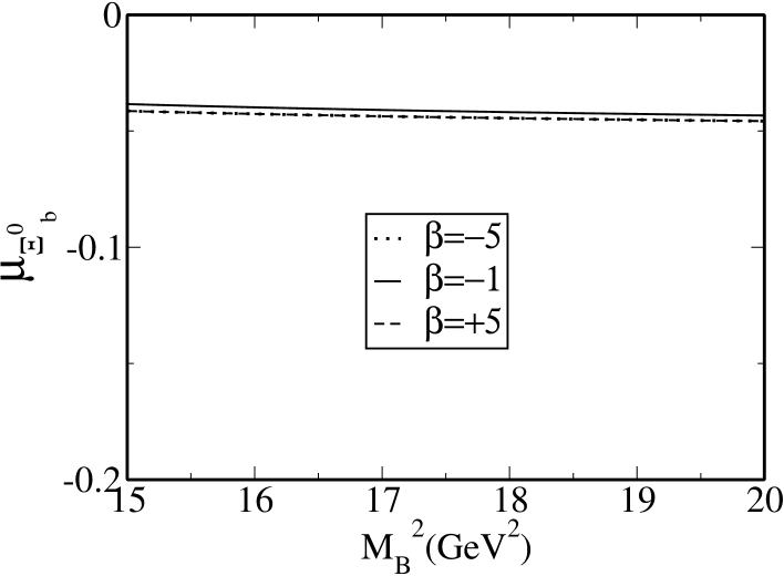
Figure 1: The dependence of magnetic moment $\mu_{\Xi_{b}^{0}}$ on $M_{B}^{2}$ at $s_{0}=6.5^{2}~{}GeV^{2}$ and $\beta=\pm 5,~{}-1$.

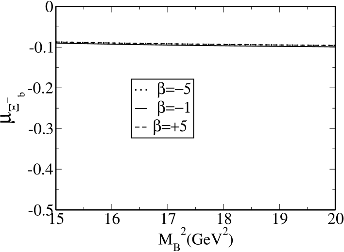
Figure 2: The same as Fig. 1 but for $\mu_{\Xi_{b}^{-}}$.

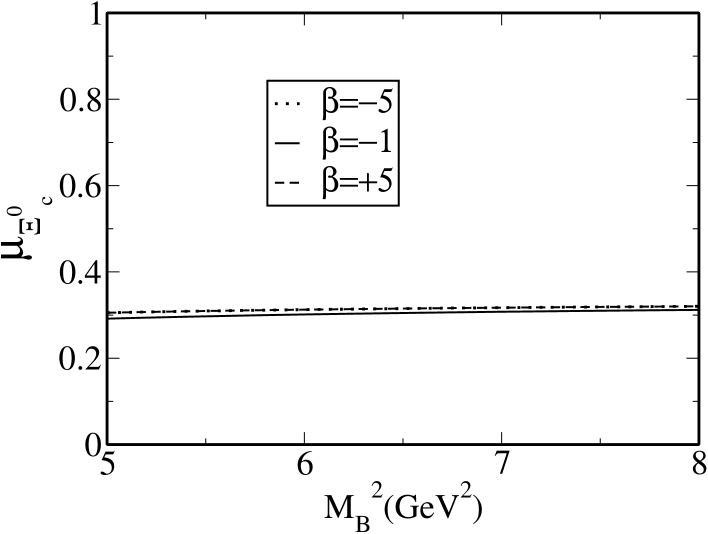
Figure 3: The same as Fig. 1 but for $\mu_{\Xi_{c}^{0}}$ and at $s_{0}=3.0^{2}~{}GeV^{2}$ .

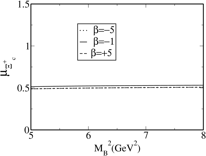
Figure 4: The same as Fig.3 but for $\mu_{\Xi_{c}^{+}}$.

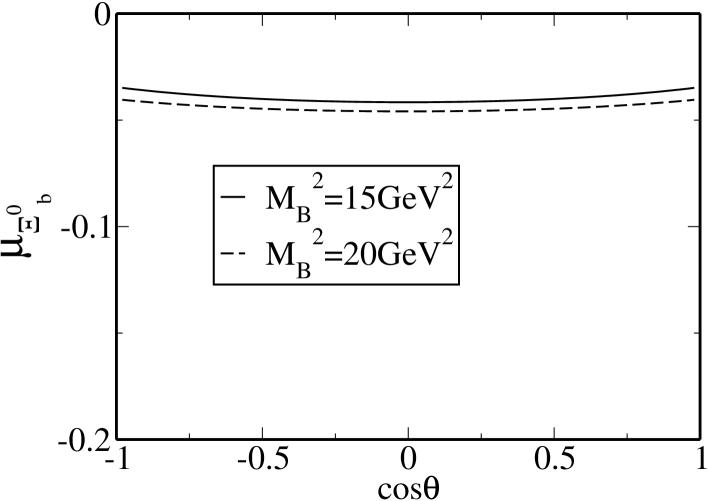
Figure 5: The dependence of the magnetic moment $\mu_{\Xi_{b}^{0}}$ on $cos\theta$ at $s_{0}=6.5^{2}~{}GeV^{2}$ and for $M_{B}^{2}=15~{}GeV^{2}$ and $M_{B}^{2}=20~{}GeV^{2}$.

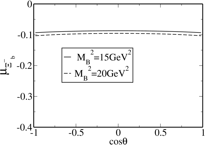
Figure 6: The same as Fig. 5 but for $\mu_{\Xi_{b}^{-}}$.

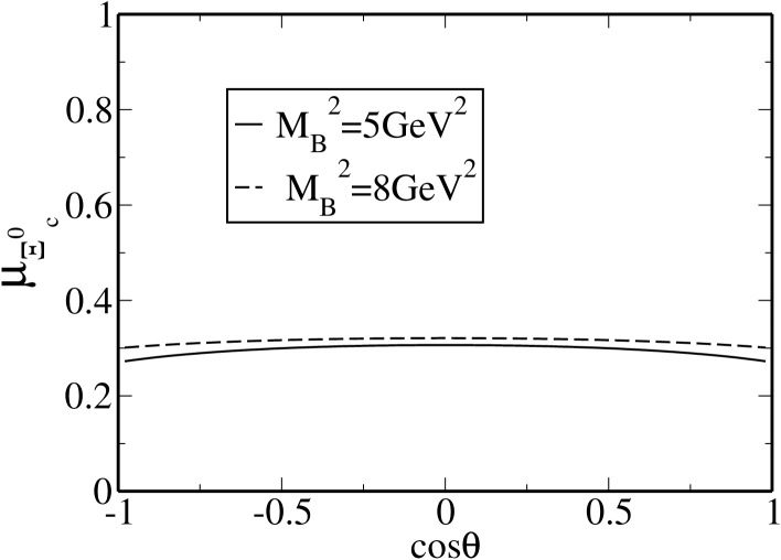
Figure 7: The same as Fig. 5 but for $\mu_{\Xi_{c}^{0}}$ and $s_{0}=3.0^{2}~{}GeV^{2}$ and for $M_{B}^{2}=5~{}GeV^{2}$ and $M_{B}^{2}=8~{}GeV^{2}$.

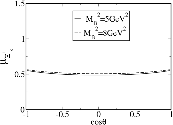
Figure 8: The same as Fig. 7 but for $\mu_{\Xi_{c}^{+}}$.

References

[1] T. Aaltonen et. al, CDF Collaboration, Phys. Rev. Lett. 99 (2007) 202001.
[2] V. Abazov et. al, DO Collaboration, Phys. Rev. Lett. 99 (2007) 052001.
[3] T. Aaltonen et. al, CDF Collaboration, Phys. Rev. Lett. 99 (2007) 052002.
[4] B. Aubert et. al, BaBar Collaboration, Phys. Rev. Lett. 97 (2006) 232001.
[5] S. Capstick, N. Isgur, Phys. Rev. D
34 (1986) 2809.
[6] R. Roncaglia, D. B. Lichtenberg, E. Predazzi, Phys. Rev.
D 52 (1995) 1722.
[7] E. Jenkins, Phys. Rev.
D 54 (1996) 4515.
[8] N. Mathur, R. Lewis , R. M. Woloshyn,
Phys. Rev. D 66 (2002) 014502.
[9] D. Ebert, R. N. Faustov, V. O. Galkin, Phys. Rev.
D 72 (2005) 034026.
[10] M. Karliner, H. J. Lipkin, arXiv:
0307343 (hep-ph), 0611306 (hep-ph).
[11] M. Karliner, B. Kereu-Zura, H. J. Lipkin, J. L. Rosner, arXiv:
0706.2163 (hep-ph).
[12] J. L. Rosner, Phys. Rev.
D 75 (2007) 013009.
[13] M. Karliner, H. J. Lipkin, Phys. Lett. B 575 (2003) 249.
[14] M. A. Shifman, A. I. Vainshtein, V. I. Zakharov,
Nucl. Phys. B 147 (1979) 385.
[15] E. Bagan, M. Chabab, H. G. Dosch, S. Narison, Phys. Lett. B 278 (1992) 367; ibid; Phys. Lett. B 287 (1992) 176; ibid;
Phys. Lett. B 301 (1993) 243.
[16] C. S. Navarra, M. Nielsen, Phys. Lett. B 443 (1998) 285.
[17] E. V. Shuryak, Nucl. Phys. B
198 (1982) 83.
[18] A. G. Grozin, O. I. Yakovlev, Phys.
Lett. B 285 (1992) 254.
[19] Y. B. Dai, C. S. Huang, C. Liu, C. D. Lu, Phys. Lett. B 371 (1996)
99.
[20] D. W. Wang, M. Q. Huang, C. Z. Li, Phys. Rev. D 65 (2002) 094036.
[21] S. L. Zhu, Phys. Rev. D 61 (2000) 114019.
[22] C. S. Huang, A. L. Zhang, S. L. Zhu, Phys. Lett. B 492 (2000)
288.
[23] D. W. Wang, M. Q. Huang, Phys. Rev. D 68 (2003) 034019.
[24] Z. G. Wang, Eur. Phys. J. C 54 (2008) 231.
[25] F. O. Duraes, M. Nielsen, Phys. Lett. B 658 (2007) 40.
[26] X. Liu, H. X. Chen, Y. R. Liu, A. Hosaka, S. L. Zhu, Phys. Rev. D 77 (2008) 014031.
[27] A. L. Choudhury, V. Joshi, Phys. Rev. D 13 (1976) 3115.
[28] D. B. Lichtenberg, Phys. Rev. D 15 (1977) 345.
[29] L. Y. Glozman, D. O. Riska, Nucl. Phys. A 603 (1996) 326.
[30] B. Julia-Diaz, D. O. Riska, Nucl. Phys. A 739 (2004) 69.
[31] S. Scholl, H. Weigel, Nucl. Phys. A 735 (2004) 163.
[32] A. Faessler et. al, Phys. Rev. D 73 (2006) 094013.
[33] B. Patel, A. K. Rai, P. C. Vinodkumar, arXiv:
0803.0221 (hep-ph).
[34] M. Savage, Phys. Lett. B 326 (1994) 303.
[35] D. O. Riska, Nucl. Instrum. Meth. B 119 (1996) 259.
[36] Y. Oh, D. P. Min, M. Rho, N. N. Scoccola, Nucl. Phys. A 534 (1991) 493.
[37] C. S. An, Nucl. Phys. A 797 (2007) 131, Erratum-ibid; A 801 (2008) 82.
[38] S. L. Zhu, W. Y. Hwang, Z. S. Yang, Phys. Rev. D 56 (1997) 7273.
[39] T. M. Aliev, A. Ozpineci, M. Savci, Phys. Rev. D 65 (2002) 096004.
[40] T. M. Aliev, A. Ozpineci, M. Savci, Phys. Rev. D 65 (2002) 056008.
[41] P. Colangelo and A.
Khodjamirian, in ”At the Frontier of Particle Physics/Handbook of
QCD”, edited by M. Shifman (World Scientific, Singapore, 2001), Vol.
3, p. 1495.
[42] V. M. Braun, Prep. arXiv:
9801222 (hep-ph).
[43] I. I. Balitsky, V. M. Braun, Nucl. Phys. B 311 (1989) 541.
[44] V. M. Braun, I. E. Filyanov, Z. Phys. C 48 (1990) 239.
[45] T. M. Aliev, A. Ozpineci, M. Savci, Phys. Rev. D 66 (2002) 016002, Erratum-ibid; D 67 (2003) 039901.
[46] P. Ball, V. M. Braun, N. Kivel, Nucl. Phys. B 649 (2003) 263.
[47] V. M. Belyaev, B. L. Ioffe, JETP 56 (1982) 493.
[48] J. Rohrwild, JHEP 0709 (2007) 073.
[49] A. E. Dorokhov, Eur. J. Phys. C 42 (2005) 309.
[50] V. M. Belyaev, I. I. Kogan, Yad. Fiz. 40 (1984) 1035.