Three-dimensional correlated-fermion phase separation from analysis of the geometric mean of the individual susceptibilities

Abstract

A quasi-Gaussian approximation scheme is formulated to study the strongly correlated imbalanced fermions thermodynamics, where the mean-field theory is not applicable. The non-Gaussian correlation effects are understood to be captured by the statistical geometric mean of the individual susceptibilities. In the three-dimensional unitary fermions ground state, an universal non-linear scaling transformation relates the physical chemical potentials with the individual Fermi kinetic energies. For the partial polarization phase separation to full polarization, the calculated critical polarization ratio is $P_{C}={[1-(1-\xi)^{6/5}]}/{[1+(1-\xi)^{6/5}]}\doteq 0.34$. The $\xi=4/9$ defines the ratio of the symmetric ground state energy density to that of the ideal fermion gas.

Phase separation resulting from the microscopic dynamics involves a wide range of natural phenomena. Currently, it also serves as the pivotal topic in the strongly interacting fermions quantum many-body theory.

In the past few years, considerable efforts understanding the crossover physics from Bardeen-Cooper-Schrieffer to Bose-Einstein condensation(BCS-BEC crossover) with ultra-cold atomic fermi gases have been made. At the Feshbach resonance point, the divergent $S$-wave scattering length with the existence of a zero-energy bound state can exhibit the thermodynamic universalityHo2004 ; Giorgini2007 .

Another exciting issue is on the asymmetric fermions phase diagram with unequal populations, which persists as a fundamental theme for a long timeSarma ; Fulde ; Larkin . With the Feshbach resonance techniques, tuning interaction strength and controlling the population or mass imbalance among the components offer a playground to test the non-perturbative many-body theory for the asymmetric fermions thermodynamicsPartridge2006 ; Zwierlein . The experiments show that at zero temperature the system can undergo a first-order quantum phase transition from a fully-paired superfluidity to a partially polarized normal gasYong2007 . Furthermore, when the imbalance population ratio $P=(N_{\uparrow}-N_{\downarrow})/(N_{\uparrow}+N_{\downarrow})$ between the two spin components reaches a critical value $P_{C}$, the state can transfer from the partially polarized phase separation to the fully polarized normal one.

The three-dimensional strongly interacting asymmetric fermions ground state is one of the prominent unresolved problemsPethick2002 . Meanwhile, the zero-temperature ground state energy of the partial polarization phase separation is of particular importance for explaining experimentsYong2007 ; Yong2008 . For the equally populated spin states, the Monte Carlo methods are believed to be capable of doing the simulation calculations. For the asymmetric system, the numerical simulations will suffer from the serious fermion sign problemBraaten2008 . Making a definitive theoretical conclusion or finding an unbiased analytical solution remains as an intriguing but herculean task. As far as we are aware, until recently, any analytical attempt was not known.

There can exist a relation between the $P_{C}$ and dimensionless constant $\xi$ at unitarity with $|a|=\infty$Cohen2005 ; reddy ; Bulgac2007 ; Yong2008 ; He2008 . The $\xi$ defines the ratio of the symmetric fermions energy density to that of the ideal noninteracting ones($T=0$). By exploring the complex non-Gaussian correlations, the purpose of this Letter is offering a novel tool to calibrate the ground state energy of strongly interacting asymmetric fermions and fix the relation between $\xi$ and $P_{C}$. The method is based on extending the formalism developed inchen2007 ; chen2008 ; chen2007-1 . The calculations are performed with $k_{B}=\hslash=1$.

To address the imbalanced fermions thermodynamics, we formulate the universal medium-scaling Hamiltonian

$$\tilde{H}= -\int d^{3}x\psi_{\alpha}^{*}(x)(\frac{\nabla^{2}}{2m_{\alpha}}-\mu_{r\alpha}[n,T])\psi_{\alpha}(x)$$ (1)

$$+\frac{U_{\mbox{eff}}^{*}[n,T]}{2}\int d^{3}x\psi_{\alpha}^{*}(x)\psi^{*}_{\beta}(x)\psi_{\beta}(x)\psi_{\alpha}(x).$$

In Eq.(1), $\alpha,\beta=\uparrow(a),\downarrow(b)$ represent the hyperfine spin projection Ising-variables. The Hamiltonian is the same as the Bethe-Peierls contact interaction, except that the bare coupling constant $U_{0}={4\pi a}/{(2m_{r})}$ is substituted by a medium regulated functional $U_{\mbox{eff}}^{*}[n,T]$. The $m_{r}={m_{a}m_{b}}/(m_{a}+m_{b})$ is the reduced mass. In the vacuum limit $n\rightarrow 0$, the $\tilde{H}$ reduces to the original version possessing a global $U(1)$ or $\mathbb{Z}_{2}$ gauge symmetry (assuming $m_{a}=m_{b}$ without a loss of generality).

Due to the medium dependence of $U_{\mbox{eff}}^{*}$, the non-trivial $\delta{\cal H}\propto\mu_{r,\alpha}[n,T]N_{\alpha}$ enforce the energy-momentum conservation lawBrown2002 . Routinely, the strong correlation effects are further understood as a spontaneously generated one-body correlation potential from the density functional theory viewpointchen2007 ; chen2008 , with which the general thermodynamic consistencies are strictly guaranteed within the non-perturbative procedures.

The medium-scaling formalism allows a natural implementation of the strong correlation physics. Initially, we need to constitute the $U_{\mbox{eff}}^{*}$ functional. The main observation is that the environment frustrating characteristic can be realized by the twisted contact interaction

$$U_{\mbox{eff}}^{*} =\frac{U_{0}}{1-\chi_{ab}U_{0}}.$$ (2)

With Eq.(2), one can define the in-medium inverse scattering length notation $a_{\mbox{eff}}$ according to $U_{\mbox{eff}}^{*}\equiv 4\pi a_{\mbox{eff}}/m$.

With the “negative” sign in the denominator of Eq.(2), the interaction is alternatively renormalized by the strong correlation effects or the background fluctuations induced in the counterpart Fermi sea. To a great extent, the susceptibility $\chi_{ab}$ is interpreted as an external field modulator simulating the mutual non-linear response. Economically, it characterizes the complications of the single particle spectrum properties and correlating couplings.

At unitarity, the scaling thermodynamic quantities depend solely on the susceptibilities. To quantify the complicated correlation effects beyond the Gaussian statistics, the global variable of interest is captured by the statistical geometric mean(instead of arithmetic mean) of the individual $\chi_{a}$ and $\chi_{b}$ for the $\uparrow$ and $\downarrow$ subsystems

$$\chi_{ab}=\sqrt{\chi_{a}\chi_{b}}.$$ (3)

The susceptibility $\chi_{i}$ itself can be separately calculated from the Lindhard correlation response function in terms of the random phase or spin “wave” approximation, which is also the final goalchen2007-1 . Alternatively, it is more convenient to calculate the susceptibility $\chi_{i}$ with the generalized Ward-Identity

$$\chi_{i}=\left(\frac{\partial n_{i}}{\partial\mu^{*}_{i}}\right)_{T}=\frac{1}{T\lambda^{3}}f_{\frac{1}{2}}(z^{\prime}_{i}),~{}~{}~{}~{}~{}i=a,b.$$ (4)

The $f_{j}(z^{\prime}_{i})$ is the Fermi integrals with $j=-\frac{1}{2},\frac{1}{2},\cdots$ and the thermodynamical de Broglie wavelength is $\lambda=\sqrt{{(2\pi)}/{mT}}$. The collective dynamical variables $\mu^{*}_{i}$ are defined by the gap equations Eqs.(7). The effective fugacity $z_{i}^{\prime}=e^{\beta\mu^{*}_{i}}$ is analogous to the fugacity $z=e^{\beta\mu}$chen2007 ; chen2008 .

At $T=0$, $\chi_{ab}$ is the density of states(DOS) geometric mean

$$\chi_{ab}=\sqrt{N(\epsilon_{a})N(\epsilon_{b})}.$$ (5)

Here, $N(\epsilon_{i})$ is the familiar un-perturbated DOS near the Fermi surface for the one component fermionsPethick2002 .

From the action Eq.(1), the grand thermodynamical potential $\Omega(T,\mu_{a},\mu_{b})$ or pressure can be presented as the coupled parametric equations with the instantaneous quasi-Gaussian approximation methodchen2007 ; chen2008

$$P =\frac{T}{\lambda^{3}}\sum_{i=a,b}f_{5/2}(z^{\prime}_{i})+\frac{4\pi a_{\mbox{eff}}}{m}n_{a}n_{b}+\sum_{i=a,b}\mu_{r,i}n_{i},$$ (6)

$$\mu_{a} =\mu^{*}_{a}+\frac{4\pi a_{\mbox{eff}}}{m}n_{b}+\mu_{r,a},~{}~{}~{}~{}\mu_{b}=\mu_{a}({a\rightleftharpoons b}).$$ (7)

The dynamical gap equations Eqs.(7) for the corresponding single particle Green function give the definition of the effective chemical potential $\mu^{*}_{i}$, respectively. The number density $n_{i}$ is expressed in terms of the defined quasi-particle Fermi-Dirac distribution function $f_{k,i}$

$$n_{i} =\frac{1}{\lambda^{3}}f_{\frac{3}{2}}(z^{\prime}_{i}),~{}~{}~{}~{}f_{k,i}=\frac{1}{z^{\prime-1}_{i}e^{\beta\frac{{\bf k}^{2}}{2m}}+1}.$$ (8)

Sticking to the effective interaction Eq.(2) renormalized by the mixing susceptibility Eq.(3) with Eq.(4), the strengths of the correction terms to the Gaussian term are self-consistently derivedchen2007 ; chen2008

$$\mu_{r,a} ={\cal C}(T,z^{\prime}_{a})\left(\frac{4\pi a_{\mbox{eff}}}{m}\right)^{2}\sqrt{\frac{\chi_{b}}{\chi_{a}}}n_{a}n_{b},$$

$$\mu_{r,b} =\mu_{r,a}(a\rightleftharpoons b),~{}~{}~{}~{}{\cal C}(T,z^{\prime}_{i})=\frac{f_{-1/2}[z^{\prime}_{i}]}{2Tf_{1/2}[z^{\prime}_{i}]}.$$

From the underlying grand thermodynamical potential Eq.(6) and with Eqs.(7), one can derive the remaining thermodynamical quantities. For example, the energy density $\epsilon=E/V$ and entropy density $s=S/V$ read

$$\epsilon =\frac{3T}{2\lambda^{3}}\sum_{i=a,b}f_{5/2}(z^{\prime}_{i})+\frac{4\pi a_{\mbox{eff}}}{m}n_{a}n_{b}+Ts_{r},$$ (9)

$$s =\frac{1}{{2T\lambda^{3}}}\sum_{i=a,b}\left(5Tf_{5/2}(z^{\prime}_{i})-2\mu^{*}_{i}f_{3/2}(z_{i}^{\prime})\right)+s_{r},$$

with

$$s_{r}=4n_{a}n_{b}\left(\frac{2\pi a_{\mbox{eff}}}{m}\right)^{2}\left[\sqrt{\frac{\chi_{b}}{\chi_{a}}}{\cal D}(T,\mu^{*}_{a})+(a\rightleftharpoons b)\right],$$

$${\cal D}(T,\mu^{*}_{i})=\frac{\left(\frac{\partial^{2}n_{i}}{\partial{\mu^{*}_{i}}^{2}}\right)_{T}\left(\frac{\partial n_{i}}{\partial T}\right)_{\mu^{*}_{i}}-\frac{\partial^{2}n_{i}}{\partial T\partial{\mu^{*}_{i}}}\left(\frac{\partial n_{i}}{\partial{\mu^{*}_{i}}}\right)_{T}}{2\left(\frac{\partial n_{i}}{\partial\mu^{*}_{i}}\right)_{T}}.$$

A few remarks are re-emphasized on the grand thermodynamical potential because it plays an important role. The $\Omega(T,\mu_{a},\mu_{b})$ is not the naive polynomial expanded according to the bare vacuum interaction strength $U_{0}$. The collective dynamical variable $\mu^{*}_{i}$ mixes the low and high order contributions. Hidden in the factors ${\cal C}(T,\mu^{*}_{i})$ and ${\cal D}(T,\mu^{*}_{i})$ as well as in $\chi_{ab}$, the collective correlations are combined with the infinite individual dynamical high order effects. The equations Eq.(6)-Eq.(7) are highly non-linear although they appear a set of coupled algebra ones. The $\mu^{*}_{i}$ dependence of $\Omega$ can be numerically eliminated in favor of the physical chemical potential $\mu_{i}$.

In the following, we will examine the zero-temperature asymmetric interacting system thermodynamics, which can be derived analytically. At $T=0$, the pressure Eq.(6) and energy density Eq.(9) expressions read

$$P =4\left(\frac{2\pi a_{eff}}{m}\right)^{2}n_{a}n_{b}\left(C(\epsilon_{a})n_{a}\sqrt{\frac{k_{b}}{k_{a}}}+(a\rightleftharpoons b)\right)$$ (10)

$$~{}~{}~{}~{}+\frac{2}{5}\sum_{i=a,b}n_{i}\epsilon_{i}+\frac{4\pi a_{eff}}{m}n_{a}n_{b},$$

$$\epsilon =\frac{3}{5}\sum_{i=a,b}n_{i}\epsilon_{i}+\frac{4\pi a_{eff}}{m}n_{a}n_{b},$$ (11)

where the “Fermi” kinetic energy $\epsilon_{i}$, particle number density $n_{i}$ and rearrangement factor $C(\epsilon_{i})$ are

$$\epsilon_{i}=\frac{k_{i}^{2}}{2m},~{}~{}~{}~{}~{}~{}~{}n_{i}=\frac{k_{i}^{3}}{6\pi^{2}},~{}~{}~{}~{}~{}~{}~{}C(\epsilon_{i})=\frac{1}{4\epsilon_{i}}.$$ (12)

The reduced chemical potentials Eq.(7) and $a_{\mbox{eff}}$ are

$$\mu_{a} =\epsilon_{a}+\frac{4\pi a_{\mbox{eff}}}{m}n_{b}+C(\epsilon_{a})\left(\frac{4\pi a_{eff}}{m}\right)^{2}\sqrt{\frac{k_{b}}{k_{a}}}n_{a}n_{b};$$

$$\mu_{b} =\mu_{a}(a\rightleftharpoons b),~{}~{}~{}~{}a_{\mbox{eff}}=\frac{a}{1-\frac{2a}{\pi}\sqrt{k_{a}k_{b}}}.$$

The $k_{i}$ is the corresponding Fermi momentum.

With unitary $a=|\infty|$, the above expressions can be further reduced to an oversimplified compact formalism

$$P=\frac{2}{5}n_{a}\mu_{a}+\frac{2}{5}n_{b}\mu_{b},~{}~{}\epsilon=\frac{3}{5}n_{a}\mu_{a}+\frac{3}{5}n_{b}\mu_{b},$$ (13)

with

$$\mu_{a}=\epsilon_{a}-\frac{5}{9}\epsilon_{b}\left(\frac{\epsilon_{b}}{\epsilon_{a}}\right)^{1/4},~{}\mu_{b}=\epsilon_{b}-\frac{5}{9}\epsilon_{a}\left(\frac{\epsilon_{a}}{\epsilon_{b}}\right)^{1/4}.$$ (14)

The salient feature of the main results Eq.(13) is that they appear as the $\uparrow(a)$ component contributions “plus” those of $\downarrow(b)$. The zero-temperature unitary fermions thermodynamics obeys the new form of universality, i.e., the Dalton partial pressure law of the non-interacting ideal gas. Implicitly, the interaction and collective correlation information is incorporated through the chemical potentials Eq.(14).

Let us further discuss the physical chemical potentials. They are related with the Fermi kinetic energies of the two subsystems through the non-linear transformations Eq.(14). With Eq.(14), the energy density and pressure can be expressed as the regular functions of the Fermi kinetic energies according to Eq.(13).

With the population imbalance polarization ratio $P$ ($0\leq P\leq 1$, assuming $n_{a}\geq n_{b}$ and $\mu_{a}\geq\mu_{b}$)

$$P=\frac{n_{a}-n_{b}}{n_{a}+n_{b}},$$ (15)

the numerical solutions of the chemical potentials are presented in Fig.1. One can see the minority chemical potential($\mu_{b}$) decreases very rapidly while crossing the transverse axis.

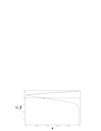
Figure 1: Rescaled chemical potentials versus $P$ at unitarity, with “+” indicating the critical position. The above curve is for the majority fermions chemical potential while the below one is for the minority component.

For $D=3$-dimensional, the reciprocal relations of the transformations Eq.(14) are very involved; i.e., it is a hard task to express the Fermi kinetic energies in terms of the chemical potentials $\mu_{a}$ and $\mu_{b}$. In principle, the Fermi kinetic energies and particle number densities in terms of the physical chemical potentials can be the functional formalisms such as $\epsilon_{a}[\mu_{a},\mu_{b},(\frac{\mu_{a}}{\mu_{b}})^{1/4}]$. In addition to the mathematical complication, the inverse transformation can be singular and nontrivial when $\mu_{b}=0$. The minority fermions chemical potential $\mu_{b}$ will change sign at this point indicated by $P_{C}$. In other words, the minority component will quickly “collapse” due to the strongly attractive interaction and the system consists of a single Fermi surface; below it, there can be two distinct Fermi surfaces and the phase separation is favoredSheehy2007 .

Namely, the vanishing $\mu_{b}$ determines the transferring criterion position from the phase separation-partial polarization to the full polarization state. The analytical relation between $P_{C}$ and $\xi$ can be derived from Eq.(14)

$$P_{C}=\frac{1-(1-\xi)^{6/5}}{1+(1-\xi)^{6/5}}.$$ (16)

With $\xi=\frac{4}{9}$, the calculated critical ratio is $P_{C}\doteq 0.34$. It is in agreement with the Monte Carlo(MC) result $P_{C}\approx 0.39$ Lobo2006 ; Pilati2008 . The mean-field theory gives $P_{C}\approx 0.93$Sheehy2007 , while the recent experimental value is $P_{C}\approx 0.36$Yong2007 .

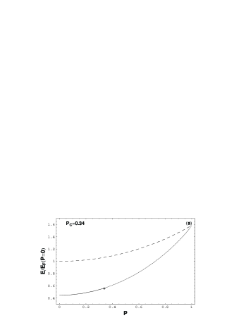
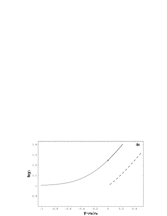
Figure 2: a), Ground state energy versus $P$ with fixed densityreddy . b), function $h(y)$ versus $y=\mu_{b}/\mu_{a}$Bulgac2007 . The dashed curve is for the non-interacting ideal Fermi gas.

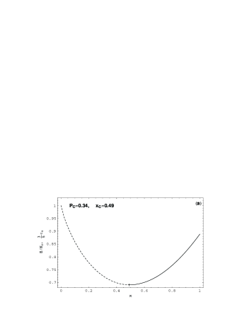
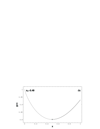
Figure 3: a), $\epsilon/(\frac{3}{5}n_{a}\epsilon_{a})$ versus $x$Lobo2006 ; b), function $g(x)$ versus $x$Yong2008 .

The complete ground state energy versus the polarization ratio $P$ is indicated in Fig. 2 and Fig.3. They are in agreement with MC calculations very wellreddy ; Lobo2006 .

For the unitary fermions ground state, the equation of state can be scaled asCohen2005 ; Yong2008 ; Bulgac2007

$$\epsilon(n_{a},n_{b}) =\frac{3(6\pi^{2})^{2/3}}{10m}\left[n_{a}g\left(\frac{n_{b}}{n_{a}}\right)\right]^{5/3},$$ (17)

$$P(\mu_{a},\mu_{b}) =\frac{(2m)^{3/2}}{15\pi^{2}}\left[\mu_{a}h\left(\frac{\mu_{b}}{\mu_{a}}\right)\right]^{5/2}$$ (18)

with the analytical scaling function

$$g(x) =(1-\frac{10}{9}x^{5/6}+x^{5/3})^{3/5}.$$ (19)

It is easy to verify that $P_{C}$ corresponds to the critical concentration defined in Refs.Yong2008 ; Lobo2006 with $x_{C}\doteq 0.49$, where the scaling $g(x)$ function takes the minimum value as indicated in Fig. 3(b). The convex behavior of $g(x)$ coincides with the experimental measurementYong2008 . The numerical solution of the $h(y)$ versus $y=\mu_{b}/\mu_{a}$ is displayed in Fig.2.b. These results contribute to understanding the realistic trapped system thermodynamics.

To conclude, the complicated non-Gaussian fluctuation and correlation effects beyond the canonical Gaussian techniques are encoded with the statistical geometric mean of the individual susceptibilities. The simple medium-renormalized effective action constitutes the bridge towards fixing the energy density functional of the strong interaction fermions system.

The non-linear scaling transformation identity Eq.(14) relates the physical chemical potentials with the Fermi kinetic energies. The reassuring association between the critical proportional ratio $P_{C}$ and universal coefficient $\xi$ agrees well with the Monte Carlo calculations and experimental measurements. This non-Gaussian correlation perspective will stimulate further insights in understanding the novel quantum phase separation dynamics.

- (1) T.-L. Ho, Phys. Rev. Lett. 92, 090402 (2004).
- (2) S. Giorgini, L.P. Pitaevskii and S. Stringari, Rev. Mod. Phys. 80, 1215 (2008) and references therein.
- (3) G. Sarma, J. Phys. Chem. Solids. 9, 266 (1962).
- (4) A.I. Larkin and Y.N. Ovchinnikovm, Phys. JETP 20, 762 (1965).
- (5) P. Fulde and R.A. Ferrell, Phys. Rev. 135, A550 (1964).
- (6) G.B. Partridge, W. Li, R.I. Kamar, Y.-A Liao, and R.G. Hulet, Science 311, 503 (2006).
- (7) M.W. Zwierlein, A. Schirotzek, C.H. Schunck and W. Ketterle, Science 311, 492 (2006).
- (8) Y.I. Shin, C.H. Schunck, A. Schirotzek and W. Ketterle, Nature 451, 689 (2008).
- (9) C.J. Pethick and H. Smith, Bose-Einstein Condensation in Dilute Gases (Cambridge University Press, Cambridge, England, 2002).
- (10) Y.I. Shin, Phys. Rev. A 77, 041603(R) (2008).
- (11) E. Braaten and L. Platter, Phys. Rev. Lett. 100, 205301 (2008).
- (12) T.D. Cohen, Phys. Rev. Lett. 95, 120403 (2005).
- (13) J. Carlson and S. Reddy, Phys. Rev. Lett. 95, 060401 (2005).
- (14) A. Bulgac and M.M. Forbes, Phys. Rev. A 75, 031605(R) (2007).
- (15) L.-Y He and P.-F Zhuang, e-print arXiv:0803.4052.
- (16) J.-S Chen, C.-M Cheng, J.-R Li, and Y.-P Wang, Phys. Rev. A 76, 033617 (2007); J.-S Chen, J.-R Li, Y.-P Wang and X.-J Xia, J. Stat. Mech. (2008) P12008.
- (17) J.-S Chen, e-print arXiv:0807.4781.
- (18) J.-S Chen, Chin. Phys. Lett. 24, 1825 (2007) and Commun. Theor. Phys. 48, 99 (2007).
- (19) G.E. Brown and M. Rho, Phys. Rep. 363, 85 (2002).
- (20) D.E. Sheehy and L. Radzihovsky, Ann. Phys. (N.Y.) 322, 1790 (2007).
- (21) C. Lobo, A. Recati, S. Giorgini, and S. Stringari, Phys. Rev. Lett. 97, 200403 (2006).
- (22) S. Pilati and S. Giorgini, Phys. Rev. Lett. 100, 030401 (2008).