Jacobi stability of the vacuum in the static spherically symmetric brane world models

Abstract

We analyze the stability of the structure equations of the vacuum in the brane world models, by using both the linear (Lyapunov) stability analysis, and the Jacobi stability analysis, the Kosambi-Cartan-Chern (KCC) theory. In the brane world models the four dimensional effective Einstein equations acquire extra terms, called dark radiation and dark pressure, respectively, which arise from the embedding of the 3-brane in the bulk. Generally, the spherically symmetric vacuum solutions of the brane gravitational field equations, have properties quite distinct as compared to the standard black hole solutions of general relativity. We close the structure equations by assuming a simple linear equation of state for the dark pressure. In this case the vacuum is Jacobi stable only for a small range of values of the proportionality constant relating the dark pressure and the dark radiation. The unstable trajectories on the brane behave chaotically, in the sense that after a finite radial distance it would be impossible to distinguish the trajectories that were very near each other at an initial point. Hence the Jacobi stability analysis offers a powerful method for constraining the physical properties of the vacuum on the brane.

I Introduction

The idea of embedding our Universe in a higher dimensional space has attracted a considerable interest recently, due to the proposal by Randall and Sundrum that our four-dimensional (4D) spacetime is a three-brane, embedded in a 5D spacetime (the bulk)  RS99a . According to the brane world scenario, the physical fields (electromagnetic, Yang-Mills etc.) in our 4D Universe are confined to the three brane. Only gravity can freely propagate in both the brane and bulk spacetimes, with the gravitational self-couplings not significantly modified. Even if the fifth dimension is uncompactified, standard 4D gravity is reproduced on the brane. Hence this model allows the presence of large, or even infinite non-compact extra dimensions. Our brane is identified to a domain wall in a 5D anti-de Sitter spacetime. In the brane world scenario, the fundamental scale of gravity is not the Planck scale, but another scale which may be at the TeV level (for a review of the dynamics and geometry of brane world models see Mart04 ). Due to the correction terms coming from the extra dimensions, significant deviations from the standard Einstein theory occur at very high energies  SMS00 . Gravity is largely modified at the electro-weak scale of about $1$ TeV. The cosmological and astrophysical implications of the brane world theories have been extensively investigated in the physical literature all2 ; sol .

The static vacuum gravitational field equations on the brane depend on the generally unknown Weyl stresses, which can be expressed in terms of two functions, called the dark radiation $U$ and the dark pressure $P$ terms (the projections of the Weyl curvature of the bulk, generating non-local brane stresses) Da00 ; Mart04 ; GeMa01 .

Several classes of spherically symmetric solutions of the static gravitational field equations in the vacuum on the brane have been obtained in Ha03 ; Ma04 ; Ha05 . As a possible physical application of these solutions the behavior of the angular velocity $v_{tg}$ of the test particles in stable circular orbits has been considered Ma04 ; Ha05 ; BoHa07 ; HaCh07 . The observed properties of the rotational galactic curves  Bi87 can be naturally explained in the brane world models, without introducing any additional hypothesis. The galaxy is embedded in a modified, spherically symmetric geometry, generated by the non-zero contribution of the Weyl tensor from the bulk. The extra terms, which can be described in terms of the dark radiation term $U$ and the dark pressure term $P$, act as a “matter” distribution outside the galaxy. The particles moving in this geometry feel the gravitational effects of $U$, which can be expressed in terms of an equivalent mass $M_{U}$ (the dark mass) Ma04 ; BoHa07 ; HaCh07 . The role of the cross-over length scale in the possible explanation of the dark-matter phenomenon in the brane world model was investigated in VySh07 . Similar interpretations of the dark matter as a bulk effect have been also considered in Pal .

For standard general relativistic spherical compact objects the exterior space-time is described by the Schwarzschild metric. In the five dimensional brane world models, the high energy corrections to the energy density, together with the Weyl stresses from bulk gravitons, imply that on the brane the exterior metric of a static star is no longer the Schwarzschild metric Da00 . The presence of the Weyl stresses also means that the matching conditions do not have a unique solution on the brane; the knowledge of the five-dimensional Weyl tensor is needed as a minimum condition for uniqueness.

Static, spherically symmetric exterior vacuum solutions of the brane world models have been obtained first in Da00 and in GeMa01 . The first of these solutions has the mathematical form of the Reissner-Nordstrom solution of the standard general relativity, in which a tidal Weyl parameter plays the role of the electric charge of the general relativistic solution Da00 . A second exterior solution, which also matches a constant density interior, has been derived in GeMa01 . Other vacuum solutions of the field equations in the brane world model have been obtained in cfm02 ; Da03 ; Vi03 ; Ca03 ; BMD03 .

Generally, the vacuum field equations on the brane can be reduced to a system of two ordinary differential equations, which describe all the geometric properties of the vacuum as functions of the dark pressure and dark radiation terms Ha03 . In order to close the system of vacuum field equations on the brane a functional relation between these two quantities is necessary.

Hence, a first possible approach to the study of the vacuum brane consists in adopting an explicit equation of state for the dark pressure as a function of the dark radiation. The explicit form of this equation can be obtained by assuming that the brane obeys different geometrical or physical conditions. The existence of the group of the homology transformations on the brane uniquely fixes the form of the equation of state Ha03 ). By assuming that the vacuum admits the group of conformal motions leads to the full determination of the equation of state of the dark pressure Ha03 ; Ma04 . By imposing the condition of the constancy of the rotational velocity curves for particle in stable orbits closes the system of the field equations, and the dark radiation and pressure can be obtained explicitly Ha03 ; Ha05 ; BoHa07 ; HaCh07 . This approach has the advantage of making predictions that may be tested directly by observations.

It is the purpose of the present paper to consider an alternative possibility for constraining the equation of state of the dark pressure on the brane. The structure equations of the vacuum can be transformed to an autonomous system of two differential equations, which in turn may be reduced to a single, second order differential equation. A second order differential equation can be investigated in geometric terms by using the general path-space theory of Kosambi-Cartan-Chern (KCC-theory) inspired by the geometry of a Finsler space Ko33 ; Ca33 ; Ch39 . The KCC theory is a differential geometric theory of the variational equations for the deviation of the whole trajectory to nearby ones. By associating a non-linear connection and a Berwald type connection to the differential system, five geometrical invariants are obtained. The second invariant gives the Jacobi stability of the system Sa05 ; Sa05a . The KCC theory has been applied for the study of different physical, biochemical or technical systems (see Sa05 ; Sa05a ; An93 ; An00 and references therein).

As a toy model for the applications of the KCC theory for the study of the Jacobi stability of the vacuum in the brane world models we consider the case of the linear equation of state for the dark pressure, $P=\gamma U$. The vacuum on the brane is Jacobi stable only for a very limited range of the proportionality constant $\gamma$, $-0.5\leq\gamma\leq 0.67$, and it is Jacobi unstable for all the other possible values of $\gamma$. Hence the natural physical requirement of Jacobi stability provides a very strong constraint on the equation of state of the dark pressure, and on the physical/geometrical properties of the model. Such a constraint cannot be obtained from the linear (Lyapunov) stability analysis, which is also considered in detail.

The present paper is organized as follows. The field equations for the vacuum on the brane are written down in Section II. The structure equations of the vacuum are derived in Section III. We review the mathematical formalism of the KCC theory in Section IV. The linear stability analysis of the structure equations of the vacuum for a linear equation of state for the dark pressure is performed in Section V. The Jacobi stability of the structure equations is analyzed in Section VI. We discuss and conclude our results in Section VII.

II The field equations for static, spherically symmetric vacuum branes

In the present Section we briefly describe the basic mathematical formalism of the brane world models, present the field equations for a static, spherically symmetric vacuum brane, and discuss some of their consequences.

II.1 The field equations in the brane world models

We start by considering a five dimensional (5D) spacetime (the bulk), with a single four-dimensional (4D) brane, on which matter is confined. The 4D brane world $({}^{(4)}M,g_{\mu\nu})$ is located at a hypersurface $\left(B\left(X^{A}\right)=0\right)$ in the 5D bulk spacetime $({}^{(5)}M,g_{AB})$, of which coordinates are described by $X^{A},A=0,1,...,4$. The induced 4D coordinates on the brane are $x^{\mu},\mu=0,1,2,3$.

The action of the system is given by SMS00

$$S=S_{bulk}+S_{brane},$$ (1)

where

$$S_{bulk}=\int_{{}^{(5)}M}\sqrt{-{}^{(5)}g}\left[\frac{1}{2k_{5}^{2}}{}^{(5)}R+{}^{(5)}L_{m}+\Lambda_{5}\right]d^{5}X,$$ (2)

and

$$S_{brane}=\int_{{}^{(4)}M}\sqrt{-{}^{(5)}g}\left[\frac{1}{k_{5}^{2}}K^{\pm}+L_{brane}\left(g_{\alpha\beta},\psi\right)+\lambda_{b}\right]d^{4}x,$$ (3)

where $k_{5}^{2}=8\pi G_{5}$ is the 5D gravitational constant, ${}^{(5)}R$ and ${}^{(5)}L_{m}$ are the 5D scalar curvature and the matter Lagrangian in the bulk, $L_{brane}\left(g_{\alpha\beta},\psi\right)$ is the 4D Lagrangian, which is given by a generic functional of the brane metric $g_{\alpha\beta}$ and of the matter fields $\psi$, $K^{\pm}$ is the trace of the extrinsic curvature on either side of the brane, and $\Lambda_{5}$ and $\lambda_{b}$ (the constant brane tension) are the negative vacuum energy densities in the bulk and on the brane, respectively.

The Einstein field equations in the bulk are given by SMS00

$${}^{(5)}G_{IJ}=k_{5}^{2}{}^{(5)}T_{IJ},\qquad{}^{(5)}T_{IJ}=-\Lambda_{5}{}^{(5)}g_{IJ}+\delta(B)\left[-\lambda_{b}{}^{(5)}g_{IJ}+T_{IJ}\right],$$ (4)

where

$${}^{(5)}T_{IJ}\equiv-2\frac{\delta{}^{(5)}L_{m}}{\delta{}^{(5)}g^{IJ}}+{}^{(5)}g_{IJ}{}^{(5)}L_{m},$$ (5)

is the energy-momentum tensor of bulk matter fields, while $T_{\mu\nu}$ is the energy-momentum tensor localized on the brane and which is defined by

$$T_{\mu\nu}\equiv-2\frac{\delta L_{brane}}{\delta g^{\mu\nu}}+g_{\mu\nu}\text{ }L_{brane}.$$ (6)

The delta function $\delta\left(B\right)$ denotes the localization of brane contribution. In the 5D spacetime a brane is a fixed point of the $Z_{2}$ symmetry. The basic equations on the brane are obtained by projections onto the brane world. The induced 4D metric is $g_{IJ}={}^{(5)}g_{IJ}-n_{I}n_{J}$, where $n_{I}$ is the space-like unit vector field normal to the brane hypersurface ${}^{(4)}M$. In the following we assume ${}^{(5)}L_{m}=0$. In the brane world models only gravity can probe the extra dimensions.

Assuming a metric of the form $ds^{2}=(n_{I}n_{J}+g_{IJ})dx^{I}dx^{J}$, with $n_{I}dx^{I}=d\chi$ the unit normal to the $\chi=\mathrm{constant}$ hypersurfaces and $g_{IJ}$ the induced metric on $\chi=\mathrm{constant}$ hypersurfaces, the effective 4D gravitational equation on the brane takes the form SMS00 :

$$G_{\mu\nu}=-\Lambda g_{\mu\nu}+k_{4}^{2}T_{\mu\nu}+k_{5}^{4}S_{\mu\nu}-E_{\mu\nu},$$ (7)

where $S_{\mu\nu}$ is the local quadratic energy-momentum correction

$$S_{\mu\nu}=\frac{1}{12}TT_{\mu\nu}-\frac{1}{4}T_{\mu}{}^{\alpha}T_{\nu\alpha}+\frac{1}{24}g_{\mu\nu}\left(3T^{\alpha\beta}T_{\alpha\beta}-T^{2}\right),$$ (8)

and $E_{\mu\nu}$ is the non-local effect from the free bulk gravitational field, the transmitted projection of the bulk Weyl tensor $C_{IAJB}$, $E_{IJ}=C_{IAJB}n^{A}n^{B}$, with the property $E_{IJ}\rightarrow E_{\mu\nu}\delta_{I}^{\mu}\delta_{J}^{\nu}\quad$as$\quad\chi\rightarrow 0$. We have also denoted $k_{4}^{2}=8\pi G$, with $G$ the usual 4D gravitational constant.

The 4D cosmological constant, $\Lambda$, and the 4D coupling constant, $k_{4}$, are related by $\Lambda=k_{5}^{2}(\Lambda_{5}+k_{5}^{2}\lambda_{b}^{2}/6)/2$ and $k_{4}^{2}=k_{5}^{4}\lambda_{b}/6$, respectively. In the limit $\lambda_{b}^{-1}\rightarrow 0$ we recover standard general relativity SMS00 .

The Einstein equation in the bulk and the Codazzi equation also imply the conservation of the energy-momentum tensor of the matter on the brane, $D_{\nu}T_{\mu}{}^{\nu}=0$, where $D_{\nu}$ denotes the brane covariant derivative. Moreover, from the contracted Bianchi identities on the brane it follows that the projected Weyl tensor obeys the constraint $D_{\nu}E_{\mu}{}^{\nu}=k_{5}^{4}D_{\nu}S_{\mu}{}^{\nu}$.

The symmetry properties of $E_{\mu\nu}$ imply that in general we can decompose it irreducibly with respect to a chosen $4$-velocity field $u^{\mu}$ as Mart04

$$E_{\mu\nu}=-k^{4}\left[U\left(u_{\mu}u_{\nu}+\frac{1}{3}h_{\mu\nu}\right)+P_{\mu\nu}+2Q_{(\mu}u_{\nu)}\right],$$ (9)

where $k=k_{5}/k_{4}$, $h_{\mu\nu}=g_{\mu\nu}+u_{\mu}u_{\nu}$ projects orthogonal to $u^{\mu}$, the “dark radiation” term $U=-k^{-4}E_{\mu\nu}u^{\mu}u^{\nu}$ is a scalar, $Q_{\mu}=k^{-4}h_{\mu}^{\alpha}E_{\alpha\beta}u^{\beta}$ is a spatial vector and $P_{\mu\nu}=-k^{-4}\left[h_{(\mu}\text{ }^{\alpha}h_{\nu)}\text{ }^{\beta}-\frac{1}{3}h_{\mu\nu}h^{\alpha\beta}\right]E_{\alpha\beta}$ is a spatial, symmetric and trace-free tensor.

In the case of the vacuum state we have $\rho=p=0$, $T_{\mu\nu}\equiv 0$, and consequently $S_{\mu\nu}\equiv 0$. Therefore the field equation describing a static brane takes the form

$$R_{\mu\nu}=-E_{\mu\nu}+\Lambda g_{\mu\nu},$$ (10)

with the trace $R$ of the Ricci tensor $R_{\mu\nu}$ satisfying the condition $R=R_{\mu}^{\mu}=4\Lambda$.

In the vacuum case $E_{\mu\nu}$ satisfies the constraint $D_{\nu}E_{\mu}{}^{\nu}=0$. In an inertial frame at any point on the brane we have $u^{\mu}=\delta_{0}^{\mu}$ and $h_{\mu\nu}=\mathrm{diag}(0,1,1,1)$. In a static vacuum $Q_{\mu}=0$ and the constraint for $E_{\mu\nu}$ takes the form  GeMa01

$$\frac{1}{3}D_{\mu}U+\frac{4}{3}UA_{\mu}+D^{\nu}P_{\mu\nu}+A^{\nu}P_{\mu\nu}=0,$$ (11)

where $A_{\mu}=u^{\nu}D_{\nu}u_{\mu}$ is the 4-acceleration. In the static spherically symmetric case we may chose $A_{\mu}=A(r)r_{\mu}$ and $P_{\mu\nu}=P(r)\left(r_{\mu}r_{\nu}-\frac{1}{3}h_{\mu\nu}\right)$, where $A(r)$ and $P(r)$ (the “dark pressure”) are some scalar functions of the radial distance $r$, and $r_{\mu}$ is a unit radial vector Da00 .

II.2 The gravitational field equations for a static spherically symmetric brane

In the following we will restrict our study to the static and spherically symmetric metric given by

$$ds^{2}=-e^{\nu(r)}dt^{2}+e^{\lambda(r)}dr^{2}+r^{2}\left(d\theta^{2}+\sin^{2}\theta d\phi^{2}\right).$$ (12)

With the metric given by (12) the gravitational field equations and the effective energy-momentum tensor conservation equation in the vacuum take the form Ha03 ; Ma04

$$-e^{-\lambda}\left(\frac{1}{r^{2}}-\frac{\lambda^{\prime}}{r}\right)+\frac{1}{r^{2}}=3\alpha U+\Lambda,$$ (13)

$$e^{-\lambda}\left(\frac{\nu^{\prime}}{r}+\frac{1}{r^{2}}\right)-\frac{1}{r^{2}}=\alpha\left(U+2P\right)-\Lambda,$$ (14)

$$\frac{1}{2}e^{-\lambda}\left(\nu^{\prime\prime}+\frac{\nu^{\prime 2}}{2}+\frac{\nu^{\prime}-\lambda^{\prime}}{r}-\frac{\nu^{\prime}\lambda^{\prime}}{2}\right)=\alpha\left(U-P\right)-\Lambda,$$ (15)

$$\nu^{\prime}=-\frac{U^{\prime}+2P^{\prime}}{2U+P}-\frac{6P}{r\left(2U+P\right)},$$ (16)

where ${}^{\prime}=d/dr$, and we have denoted $\alpha=16\pi G/k^{4}\lambda_{b}$.

The field equations (13)–(16) can be interpreted as describing an isotropic ”matter distribution”, with the effective energy density $\rho^{\mathrm{eff}}$, radial pressure $P^{\mathrm{eff}}$ and orthogonal pressure $P_{\perp}^{\mathrm{eff}}$, respectively, so that $\rho^{\mathrm{eff}}=3\alpha U+\Lambda$, $P^{\mathrm{eff}}=\alpha U+2\alpha P-\Lambda$ and $P_{\perp}^{\mathrm{eff}}=\alpha U-\alpha P-\Lambda$, respectively, which gives the condition $\rho^{\mathrm{eff}}-P^{\mathrm{eff}}-2P_{\perp}^{\mathrm{eff}}=4\Lambda=\mathrm{constant}$. This is expected for the ‘radiation’ like source, for which the projection of the bulk Weyl tensor is trace-less, $E_{\mu}^{\mu}=0$.

III Structure equations of the vacuum in the brane world models

Eq. (13) can immediately be integrated to give

$$e^{-\lambda}=1-\frac{C_{1}}{r}-\frac{GM_{U}\left(r\right)}{r}-\frac{\Lambda}{3}r^{2},$$ (17)

where $C_{1}$ is an arbitrary constant of integration, and we denoted

$$GM_{U}\left(r\right)=3\alpha\int_{0}^{r}U(r)r^{2}dr.$$ (18)

The function $M_{U}$ is the gravitational mass corresponding to the dark radiation term (the dark mass). For $U=0$ the metric coefficient given by Eq. (17) must tend to the standard general relativistic Schwarzschild metric coefficient, which gives $C_{1}=2GM$, where $M=\mathrm{constant}$ is the baryonic (usual) mass of the gravitating system.

By substituting $\nu^{\prime}$ given by Eq. (16) into Eq. (2) and with the use of Eq. (17) we obtain the following system of differential equations satisfied by the dark radiation term $U$, the dark pressure $P$ and the dark mass $M_{U}$, describing the vacuum gravitational field, exterior to a massive body, in the brane world model Ha03 :

$$\frac{dM_{U}}{dr}=\frac{3\alpha}{G}r^{2}U.$$ (19)

$$\frac{dU}{dr}=-\frac{\left(2U+P\right)\left[2GM+GM_{U}-\frac{2}{3}\Lambda r^{3}+\alpha\left(U+2P\right)r^{3}\right]}{r^{2}\left(1-\frac{2GM}{r}-\frac{M_{U}}{r}-\frac{\Lambda}{3}r^{2}\right)}-2\frac{dP}{dr}-\frac{6P}{r},$$ (20)

To close the system a supplementary functional relation between one of the unknowns $U$, $P$ and $M_{U}$ is needed. Generally, this equation of state is given in the form $P=P(U)$. Once this relation is known, Eqs. (19)–(20) give a full description of the geometrical properties of the vacuum on the brane.

In the following we will restrict our analysis to the case $\Lambda=0$. Then the system of equations (19) and (20) can be transformed to an autonomous system of differential equations by means of the transformations

$$q=\frac{2GM}{r}+\frac{GM_{U}}{r},\qquad\mu=3\alpha r^{2}U,$$ (21)

$$p=3\alpha r^{2}P,\qquad\theta=\ln r,$$ (22)

where $\mu$ and $p$ are the “reduced” dark radiation and pressure, respectively.

With the use of the new variables given by Eqs. (21) and (22), Eqs. (19) and (20) become

$$\frac{dq}{d\theta}=\mu-q,$$ (23)

$$\frac{d\mu}{d\theta}=-\frac{\left(2\mu+p\right)\left[q+\frac{1}{3}\left(\mu+2p\right)\right]}{1-q}-2\frac{dp}{d\theta}+2\mu-2p.$$ (24)

Eqs. (19) and (20), or, equivalently, (23) and (24), are called the structure equations of the vacuum on the brane Ha03 . In order to close the system of equations (23) and (24) an “equation of state” $p=p\left(\mu\right)$, relating the reduced dark radiation and the dark pressure terms, is needed.

The structure equations of the vacuum on the brane can be solved exactly in two cases, corresponding to some simple equations of state of the dark pressure. In the first case we impose the equation of state $2\mu+p=0$. From Eq. (24) we immediately obtain $\mu=Qe^{-2\theta}$, while Eq. (23) gives $q\left(\theta\right)=-Qe^{-2\theta}+U_{0}e^{-\theta}$, where $Q$ and $U_{0}=2GM$ are arbitrary constants of integration. Therefore we obtain the vacuum brane solution

$$U=-\frac{P}{2}=\frac{Q}{3\alpha}\frac{1}{r^{4}},$$ (25)

$$e^{-\lambda}=e^{\nu}=1-\frac{2GM}{r}+\frac{Q}{r^{2}}.$$ (26)

This solution was first obtained in Da00 , and therefore corresponds to an equation of state of the dark pressure of the form $P=-2U$. The second case in which the vacuum structure equations can be integrated exactly corresponds to the equation of state $\mu+2p=0$. Then Eq. (24) gives $q=2/3$, and the corresponding solution of the gravitational field equations on the brane is Ha03

$$U=-2P=\frac{2}{9\alpha r^{2}},e^{\nu}=C_{0}r^{2},e^{-\lambda}=\frac{1}{3}.$$ (27)

This solution corresponds to an equation of state of the dark pressure of the form $P=-U/2$.

IV Kosambi-Cartan-Chern (KCC) theory and Jacobi stability

We recall the basics of KCC-theory to be used in the sequel. Our exposition follows Sa05 .

Let $\mathcal{M}$ be a real, smooth $n$-dimensional manifold and let $T\mathcal{M}$ be its tangent bundle. Let $\left(x^{i}\right)=\left(x^{1},x^{2},...,x^{n}\right)$, $\left(y^{i}\right)=\left(y^{1},y^{2},...,y^{n}\right)$ and the time $t$ be a $2n+1$ coordinates system of an open connected subset $\Omega$ of the Euclidian $(2n+1)$ dimensional space $R^{n}\times R^{n}\times R^{1}$, where

$$y^{i}=\left(\frac{dx^{1}}{dt},\frac{dx^{2}}{dt},...,\frac{dx^{n}}{dt}\right).$$ (28)

We assume that $t$ is an absolute invariant, and therefore the only admissible change of coordinates will be

$$\tilde{t}=t,\tilde{x}^{i}=\tilde{x}^{i}\left(x^{1},x^{2},...,x^{n}\right),i\in\left\{1,2,...,n\right\}.$$ (29)

The equations of motion of a dynamical system can be derived from a Lagrangian $L$ via the Euler-Lagrange equations,

$$\frac{d}{dt}\frac{\partial L}{\partial y^{i}}-\frac{\partial L}{\partial x^{i}}=F_{i},i=1,2,...,n,$$ (30)

where $F_{i}$, $i=1,2,...,n$, is the external force MHSS . The triplet $\left(M,L,F_{i}\right)$ is called a Finslerian mechanical system MiFr05 . For a regular Lagrangian $L$, the Euler-Lagrange equations given by Eq. (30) are equivalent to a system of second-order differential equations

$$\frac{d^{2}x^{i}}{dt^{2}}+2G^{i}\left(x^{j},y^{j},t\right)=0,i\in\left\{1,2,...,n\right\},$$ (31)

where each function $G^{i}\left(x^{j},y^{j},t\right)$ is $C^{\infty}$ in a neighborhood of some initial conditions $\left(\left(x\right)_{0},\left(y\right)_{0},t_{0}\right)$ in $\Omega$. The system given by Eq. (31) is equivalent to a vector field (semispray) $S$, where

$$S=y^{i}\frac{\partial}{\partial x^{i}}-2G^{i}\left(x^{j},y^{j},t\right)\frac{\partial}{\partial y^{i}},$$ (32)

which determines a non-linear connection $N_{j}^{i}$ defined as MHSS

$$N_{j}^{i}=\frac{\partial G^{i}}{\partial y^{j}}.$$ (33)

More generally, one can start from an arbitrary system of second-order differential equations on the form (31), where no a priori given Lagrangean function is assumed, and study the behavior of its trajectories by analogy with the trajectories of the Euler-Lagrange equations.

For a non-singular coordinate transformations given by Eq. (29), we define the KCC-covariant differential of a vector field $\xi^{i}(x)$ on the open subset $\Omega\subseteq R^{n}\times R^{n}\times R^{1}$ as An93 ; An00 ; Sa05 ; Sa05a

$$\frac{D\xi^{i}}{dt}=\frac{d\xi^{i}}{dt}+N_{j}^{i}\xi^{j}.$$ (34)

For $\xi^{i}=y^{i}$ we obtain

$$\frac{Dy^{i}}{dt}=N_{j}^{j}y^{j}-2G^{i}=-\epsilon^{i},$$ (35)

where the contravariant vector field $\epsilon^{i}$ on $\Omega$ is called the first KCC invariant.

Let us now vary the trajectories $x^{i}(t)$ of the system (31) into nearby ones according to

$$\tilde{x}^{i}\left(t\right)=x^{i}(t)+\eta\xi^{i}(t),$$ (36)

where $\left|\eta\right|$ is a small parameter and $\xi^{i}(t)$ are the components of some contravariant vector field defined along the path $x^{i}(t)$. Substituting Eqs. (36) into Eqs. (31) and taking the limit $\eta\rightarrow 0$ we obtain the variational equations An93 ; An00 ; Sa05 ; Sa05a

$$\frac{d^{2}\xi^{i}}{dt^{2}}+2N_{j}^{i}\frac{d\xi^{j}}{dt}+2\frac{\partial G^{i}}{\partial x^{j}}\xi^{j}=0.$$ (37)

By using the KCC-covariant differential we can write Eq. (37) in the covariant form

$$\frac{D^{2}\xi^{i}}{dt^{2}}=P_{j}^{i}\xi^{j},$$ (38)

where we have denoted

$$P_{j}^{i}=-2\frac{\partial G^{i}}{\partial x^{j}}-2G^{l}G_{jl}^{i}+y^{l}\frac{\partial N_{j}^{i}}{\partial x^{l}}+N_{l}^{i}N_{j}^{l}+\frac{\partial N_{j}^{i}}{\partial t},$$ (39)

and $G_{jl}^{i}\equiv\partial N_{j}^{i}/\partial y^{l}$ is called the Berwald connection An93 ; MHSS ; Sa05 ; Sa05a . Eq. (38) is called the Jacobi equation, and $P_{j}^{i}$ is called the second KCC-invariant or the deviation curvature tensor. When the system (31) describes the geodesic equations in either Riemann or Finsler geometry, Eq. (38) is the Jacobi field equation.

The third, fourth and fifth invariants of the system (31) are given by An00

$$P_{jk}^{i}\equiv\frac{1}{3}\left(\frac{\partial P_{j}^{i}}{\partial y^{k}}-\frac{\partial P_{k}^{i}}{\partial y^{j}}\right),P_{jkl}^{i}\equiv\frac{\partial P_{jk}^{i}}{\partial y^{l}},D_{jkl}^{i}\equiv\frac{\partial G_{jk}^{i}}{\partial y^{l}}.$$ (40)

The third invariant is interpreted as a torsion tensor, while the fourth and fifth invariants are the Riemann-Christoffel curvature tensor, and the Douglas tensor, respectively An00 . In a Berwald space these tensors always exist, and they describe the geometrical properties of a system of second-order differential equations.

In many physical applications we are interested in the behavior of the trajectories of the system (31) in a vicinity of a point $x^{i}\left(t_{0}\right)$, where for simplicity one can take $t_{0}=0$. We will consider the trajectories $x^{i}=x^{i}(t)$ as curves in the Euclidean space $\left(R^{n},\left\langle.,.\right\rangle\right)$, where $\left\langle.,.\right\rangle$ is the canonical inner product of $R^{n}$. As for the deviation vector $\xi$ we assume that it satisfies the initial conditions $\xi\left(0\right)=O$ and $\dot{\xi}\left(0\right)=W\neq O$, where $O\in R^{n}$ is the null vector Sa05 ; Sa05a .

For any two vectors $X,Y\in R^{n}$ we define an adapted inner product $\left\langle\left\langle.,.\right\rangle\right\rangle$ to the deviation tensor $\xi$ by $\left\langle\left\langle X,Y\right\rangle\right\rangle:=1/\left\langle W,W\right\rangle\cdot\left\langle X,Y\right\rangle$. We also have $\left|\left|W\right|\right|^{2}:=\left\langle\left\langle W,W\right\rangle\right\rangle=1$.

Thus, the focusing tendency of the trajectories around $t_{0}=0$ can be described as follows: if $\left|\left|\xi\left(t\right)\right|\right|<t^{2}$, $t\approx 0^{+}$, the trajectories are bunching together, while if $\left|\left|\xi\left(t\right)\right|\right|>t^{2}$, $t\approx 0^{+}$, the trajectories are dispersing Sa05 ; Sa05a . In terms of the deviation curvature tensor the focusing tendency of the trajectories can be described as follows: The trajectories of the system of equations (31) are bunching together for $t\approx 0^{+}$ if and only if the real part of the eigenvalues of $P_{j}^{i}\left(0\right)$ are strictly negative, and they are dispersing if and only if the real part of the eigenvalues of $P_{j}^{i}\left(0\right)$ are strict positive Sa05 ; Sa05a .

Based on these considerations we can define the Jacobi stability for a dynamical system as follows An00 ; Sa05 ; Sa05a :

Definition: If the system of differential equations (31) satisfies the initial conditions $\left|\left|x^{i}\left(t_{0}\right)-\tilde{x}^{i}\left(t_{0}\right)\right|\right|=0$, $\left|\left|\dot{x}^{i}\left(t_{0}\right)-\tilde{x}^{i}\left(t_{0}\right)\right|\right|\neq 0$, with respect to the norm $\left|\left|.\right|\right|$ induced by a positive definite inner product, then the trajectories of (31) are Jacobi stable if and only if the real parts of the eigenvalues of the deviation tensor $P_{j}^{i}$ are strictly negative everywhere, and Jacobi unstable, otherwise.

The focussing behavior of the trajectories near the origin is represented in Fig. 1.

Figure 1: Behavior of trajectories near zero.

V Linear stability analysis of the vacuum structure equations on the brane for the linear equation of state of the dark pressure

Since generally the structure equations of the vacuum on the brane cannot be solved exactly, in this Section we shall analyze them by using methods from the qualitative analysis of dynamical systems BoHa07 , by closely following the approach of  boyce . We consider the case in which the dark pressure is proportional to the dark radiation, $P=\gamma U$, where $\gamma$ is an arbitrary constant, which can take both positive and negative values. As we have seen in Section III, several classes of exact solutions of the vacuum gravitational field equations on the brane can be described by an equation of state of this form. In the reduced variables $\mu$ and $p$ the linear equation of state is $p=\gamma\mu$, and the structure equations of the gravitational field on the brane have the form

$$\frac{dq}{d\theta}=\mu-q,$$ (41)

$$\left(1+2\gamma\right)\frac{d\mu}{d\theta}=2\left(1-\gamma\right)\mu-\frac{\left(\gamma+2\right)\mu\left[q+\frac{1+2\gamma}{3}\mu\right]}{1-q}.$$ (42)

Let us firstly analyze the special case where $\gamma=-1/2$. Then, by virtue of the second Eq. (42), we obtain two possible exact solutions, either $q=\mu=0$ or $q=\mu=2/3$. The first of these solutions correspond to the vanishing of all physical quantities, and therefore we can discard it as unphysical. The second case corresponds to an exact solution, which has been discussed in Section III.

Let us henceforth assume that $\gamma\neq-1/2$, and rewrite the system of equation into the following form,

$$\frac{dq}{d\theta}=-q+\mu,$$ (43)

$$\frac{d\mu}{d\theta}=\frac{2(1-\gamma)}{1+2\gamma}\mu-\frac{\gamma+2}{1+2\gamma}\frac{\mu\left[q+\frac{1+2\gamma}{3}\mu\right]}{1-q},$$ (44)

which is finally written as

$$\frac{d\xi}{d\theta}=A\xi+B,$$ (45)

where we have denoted

$$\xi=\begin{pmatrix}q\\ \mu\end{pmatrix},\quad A=\begin{pmatrix}-1&1\\ 0&2(1-\gamma)/(1+2\gamma)\end{pmatrix},\quad B=\begin{pmatrix}0\\ \frac{\gamma+2}{1+2\gamma}\frac{\mu\left[q+\frac{1+2\gamma}{3}\mu\right]}{1-q}\end{pmatrix}$$ (46)

The system of equations (45) has two critical points, $X_{0}=(0,0)$, and

$$X_{\gamma}=\left(\frac{3(1-\gamma)}{\gamma^{2}+\gamma+7},\frac{3(1-\gamma)}{\gamma^{2}+\gamma+7}\right).$$ (47)

For $\gamma=1$, the two critical points of the system coincide. Depending on the values of $\gamma$, these points lie in different regions of the phase space plane $(q,\mu)$.

Since the term $||B||/||\xi||\rightarrow 0$ as $||\xi||\rightarrow 0$, the system of equations (45) can be linearized at the critical point $X_{0}$. The two eigenvalues of the matrix $A$ are given by $r_{1}=-1$ and $r_{2}=2(1-\gamma)/(1+2\gamma)$, and determine the characteristics of the critical point $X_{0}$. For $\gamma\in(-\infty,-1/2)\cup[1,\infty)$ both eigenvalues are negative and unequal. Therefore, for such values of $\gamma$ the point $X_{0}$ is an improper asymptotically stable node.

If $\gamma\in(-1/2,1)$, we find one positive and one negative eigenvalue, which corresponds to an unstable saddle point at the point $X_{0}$. Moreover, since the matrix $dA/d\xi(X_{0})$ has real non-vanishing eigenvalues, the point $X_{0}$ is hyperbolic. This implies that the properties of the linearized system are also valid for the full non-linear system near the point $X_{0}$. It should be mentioned however, that this first critical point is the less interesting one from a physical point of view, since it corresponds to the ‘trivial’ case where both physical variables vanish.

As we have seen in Section III, the structure equations can also be solved exactly for the value $\gamma=-2$. In that case, the non-linear term $B$ in Eq. (45) identically vanishes, and the system of equations becomes a simple linear system of differential equations. For $\gamma=-2$ the two eigenvalues of $A$ are given by $r_{1}=-1$ and $r_{2}=-2$, and the two corresponding eigenvectors are linearly independent. The general solution can be written as follows

$$\xi_{\gamma=-2}=(q_{0}+\mu_{0})\begin{pmatrix}1\\ 0\end{pmatrix}e^{-\theta}+\mu_{0}\begin{pmatrix}-1\\ 1\end{pmatrix}e^{-2\theta},$$ (48)

where $q_{0}=q(0)$ and $\mu_{0}=\mu(0)$. One can easily transform this solution back into the radial coordinate $r$ form by using $\theta=\ln(r)$, thus obtaining

$$\mu_{\gamma=-2}=\frac{\mu_{0}}{r^{2}},\quad q_{\gamma=-2}=\frac{q_{0}}{r}+\mu_{0}\left(\frac{1}{r}-\frac{1}{r^{2}}\right).$$ (49)

Let us now analyze the qualitative behavior of the second critical point $X_{\gamma}$. To do this, one has to Taylor expand the right-hand sides of Eqs. (43) and (44) around $X_{\gamma}$ and obtain the matrix $\tilde{A}$ which corresponds to the system, linearized around $X_{\gamma}$. This linearization is again allowed since the resulting non-linear term, $\tilde{n}$ say, also satisfies the condition $||\tilde{n}||/||\xi||\rightarrow 0$ as $||\xi||\rightarrow X_{\gamma}$. The resulting matrix reads

$$\tilde{A}=\begin{pmatrix}-1&1\\ \frac{3(-\gamma^{2}+5\gamma-4)}{(2+\gamma)^{2}(1+2\gamma)}&\frac{\gamma-1}{2+\gamma}\end{pmatrix},$$ (50)

and its two eigenvalues are given by

$$r_{\pm}=\frac{-3-6\gamma\pm\sqrt{16\gamma^{4}+8\gamma^{3}+132\gamma^{2}-28\gamma-47}}{4\gamma^{2}+10\gamma+4}.$$ (51)

For $-0.5<\gamma<0.674865$ the argument of the square root becomes negative and the eigenvalues complex. Moreover, the values $\gamma=-1/2$ and $\gamma=-2$ have to be excluded, since the eigenvalues in Eq. (50) are not defined in these cases. However, both cases have been treated separately above.

If $\gamma\in(-\infty,-1/2)\cup(1,\infty)$, then $X_{\gamma}$ corresponds to an unstable saddle point and for $\gamma\in(0.674865,1)$ it corresponds to an asymptotically stable improper node. More interesting is the parameter range $\gamma\in(-1/2,0.674865)$, where the eigenvalues become complex, however, their real parts are negative definite. Hence, for those values we find an asymptotically stable spiral point at $X_{\gamma}$. Since this point is also a hyperbolic point, the described properties are also valid for the non-linear system near that point.

$\gamma$	$-\infty$		-0.5		0.67		1		+$\infty$
$r_{\pm}$		real	—	complex	—	real	—	real
			—	Re $r_{\pm}<0$	—		—
$r_{+}$		+	—		—	–	—	–
$r_{-}$		–	—		—	–	—	+
$X_{\gamma}$		Saddle	—	Stable spiral	—	Stable node	—	Saddle

Table 1: Linear stability of the stable point $X_{\gamma}$.

The behavior of the trajectories is shown, for $\gamma=-1$ and $\gamma=0.4$, in Fig. 2. The figures show the attracting or repelling character of the steady states, respectively. The results of the linear stability analysis of the critical points $X_{\gamma}$ are summarized in Table 1.

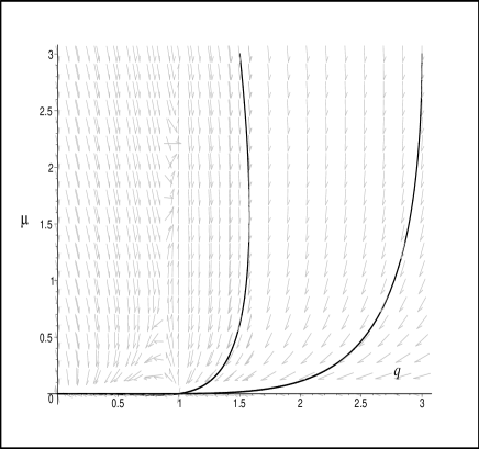
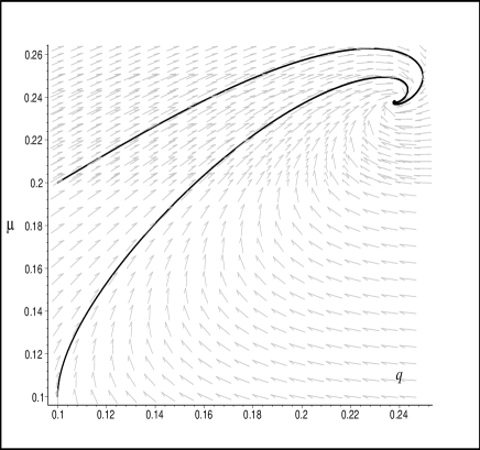
Figure 2: Behavior of the trajectories of the structure equations of the vacuum on the brane near the critical points for $\gamma=-1$ (left figure) and $\gamma=0.4$ (right figure).

VI Jacobi stability analysis of the vacuum gravitational field equations in the brane world models

Since from Eq. (41) we can express $\mu$ as $\mu=q+dq/d\theta$, upon substitution in Eq. (42) we obtain for $q$ the following second order differential equation

$$\begin{split}\frac{d^{2}q}{d\theta^{2}}&+\frac{1}{3\left(1+2\gamma\right)\left(1-q\right)}\Bigl{[}6\left(\gamma-1\right)q+2\left(\gamma^{2}+\gamma+7\right)q^{2}+3\left(4\gamma-1\right)\frac{dq}{d\theta}\\ &+\left(4\gamma^{2}+\gamma+13\right)q\frac{dq}{d\theta}+\left(2\gamma^{2}+5\gamma+2\right)\left(\frac{dq}{d\theta}\right)^{2}\Bigr{]}=0,\end{split}$$ (52)

which can now be studied by means of KCC theory.

By denoting $x=q$ and $dq/d\theta=dx/d\theta=y$, Eq. (52) can be written as

$$\frac{d^{2}x}{d\theta^{2}}+2G^{1}\left(x,y\right)=0,$$ (53)

where

$$\begin{split}G^{1}\left(x,y\right)&=\frac{1}{6\left(1+2\gamma\right)\left(1-x\right)}\Bigl{[}6\left(\gamma-1\right)x+2\left(\gamma^{2}+\gamma+7\right)x^{2}+3\left(4\gamma-1\right)y\\ &+\left(4\gamma^{2}+\gamma+13\right)xy+\left(2\gamma^{2}+5\gamma+2\right)y^{2}\Bigr{]}\end{split}$$ (54)

As a first step in the KCC stability analysis of the vacuum field equations on the brane we obtain the nonlinear connection $N_{1}^{1}$ associated to Eq. (52), and which is given by

$$N_{1}^{1}=\frac{\partial G^{1}}{\partial y}=\frac{3\left(4\gamma-1\right)+\left(4\gamma^{2}+\gamma+13\right)x+2\left(2\gamma^{2}+5\gamma+2\right)y}{6\left(1+2\gamma\right)\left(1-x\right)}.$$ (55)

The Berwald connection can be obtained as

$$G_{11}^{1}=\frac{\partial N_{1}^{1}}{\partial y}=\frac{2\gamma^{2}+5\gamma+2}{3\left(1+2\gamma\right)\left(1-x\right)}.$$ (56)

Finally, the second KCC invariant or the deviation curvature tensor $P_{1}^{1}$, defined as

$$P_{1}^{1}=-2\frac{\partial G^{1}}{\partial x}-2G^{1}G_{11}^{1}+y\frac{\partial N_{1}^{1}}{\partial x}+N_{1}^{1}N_{1}^{1},$$ (57)

reads now

$$P_{1}^{1}\left(x,y\right)=\frac{27-2\left[61+57\gamma+4\gamma^{2}\left(9+2\gamma\right)\right]x+3\left(5+\gamma\right)^{2}x^{2}-2\left(2+\gamma\right)\left(1+2\gamma\right)\left(5+4\gamma\right)y}{12\left(1-x\right)^{2}\left(1+2\gamma\right)^{2}}.$$ (58)

Taking into account that $x=q$ and $y=\mu-q$, we obtain $P_{1}^{1}$ in the initial variables as

$$P_{1}^{1}\left(q,\mu\right)=\frac{27-6\left(17+8\gamma+2\gamma^{2}\right)q+3\left(5+\gamma\right)^{2}q^{2}-2\left(2+\gamma\right)\left(1+2\gamma\right)\left(5+4\gamma\right)\mu}{12\left(1-q\right)^{2}\left(1+2\gamma\right)^{2}}.$$ (59)

Evaluating $P_{1}^{1}\left(q,\mu\right)$ at the critical point $X_{\gamma}$, given by Eq. (47), ew obtain

$$P_{1}^{1}\left(X_{\gamma}\right)=\frac{8\gamma^{3}+66\gamma-47}{4\left(2+\gamma\right)^{2}\left(1+2\gamma\right)}.$$ (60)

The plot of the function $P_{1}^{1}\left(X_{\gamma}\right)$ is represented in Fig. 3.

Figure 3: The deviation curvature tensor $P_{1}^{1}\left(X_{\gamma}\right)$ as a function of $\gamma$.

Using the discussion of Section V, our main results on the Linear stability and Jacobi stability of the critical point $X_{\gamma}$ of the vacuum field equations in the brane world models can be summarized in Table 2.

$\gamma$	$-\infty$		-0.5		0.67		1		+$\infty$
$P_{1}^{1}(X_{\gamma})$		+	—	–	—	+	—	+
Linear stability		Saddle	—	Stable	—	Stable	—	Saddle
of $X_{\gamma}$		point	—	spiral	—	node	—	point
Jacobi stability		Jacobi	—	Jacobi	—	Jacobi	—	Jacobi
of $X_{\gamma}$		unstable	—	stable	—	unstable	—	unstable

Table 2: Linear and Jacobi stability of the stable point $X_{\gamma}$.

VII Discussions and final remarks

In the present paper we have considered the stability properties of the vacuum gravitational field equations in the brane world models. For the analysis of the stability we have used two methods, the Lyapunov (linear) stability analysis, and the so-called Jacobi stability analysis, or the KCC theory. The study of the stability has been done by analyzing the behavior of the steady state $X_{\gamma}$ of the structure equations of the vacuum on the brane. The Lyapunov stability analysis involves the linearization of the dynamical system via the Jacobian matrix of a non-linear system, while the KCC theory addresses the Lyapunov stability of a whole trajectory in a tubular region Sa05 .

By using the KCC theory we have shown that the vacuum on the brane is Jacobi unstable for most of the values of the parameter $\gamma$. The stability region is reduced to a very narrow range of $\gamma$, $\gamma\in\left(-0.5,0.67\right)$. For all other values of $\gamma$ the vacuum on the brane is unstable, in the sense that the trajectories of the structure equations will disperse when approaching the origin of the coordinate system.

In a previous paper (Sa05 ) we have regarded the Jacobi stability of a dynamical system as the robustness of the system to small perturbations of the whole trajectory. This is a very convenable way of regarding the resistance of limit cycles to small perturbation of trajectories. On the other hand, we may regard the Jacobi stability for other types of dynamical systems (like the one in the present paper) as the resistance of a whole trajectory to the onset of chaos due to small perturbations of the whole trajectory. This interpretation is based on the generally accepted definition of chaos, namely a compact manifold $M$ on which the geodesic trajectories deviate exponentially fast. This is obviously related to the curvature of the base manifold (see section IV). The Jacobi (in)stability is a natural generalization of the (in)stability of the geodesic flow on a differentiable manifold endowed with a metric (Riemannian or Finslerian) to the non-metric setting. In other words, we may say that Jacobi unstable trajectories of a dynamical system behave chaotically in the sense that after a finite interval of time it would be impossible to distinguish the trajectories that were very near each other at an initial moment.

We have found that there is a good correlation between the linear stability of the critical point $X_{\gamma}$ and the robustness of the corresponding trajectory to small perturbations. Indeed, for small values of the parameter $\gamma$ the saddle point is also Jacobi unstable ($\gamma<-0.5$ and $\gamma>1$), while the stable spiral obtained for $-0.5<\gamma<0.674865$ is also robust to a small perturbation of all trajectories.

It is interesting to remark that for the interval $0.674865<\gamma<1$, the stable node is actually Jacobi unstable. In other words, even the system trajectories are attracted by the critical point $X_{\gamma}$ one has to be aware of the fact that they are not stable to small perturbation of the whole trajectory. This means that one might witness chaotic behavior of the system trajectories before they enters in a neighborhood of $X_{\gamma}$. We have here a sort of stability artifact that cannot be found without using the powerful method of Jacobi stability analysis.

- (1) L. Randall and R. Sundrum, Phys. Rev. Lett. 83, 3370 (1999); L. Randall and R. Sundrum, Phys. Rev. Lett. 83, 4690 (1999).
- (2) R. Maartens, Living Reviews in Relativity 7, 1 (2004).
- (3) M. Sasaki, T. Shiromizu and K. Maeda, Phys. Rev. D62, 024008 (2000); T. Shiromizu, K. Maeda and M. Sasaki, Phys. Rev. D62, 024012 (2000); K. Maeda, S. Mizuno and T. Torii, Phys. Rev. D68, 024033 (2003).
- (4) R. Maartens, Phys. Rev. D62, 084023 (2000); A. Campos and C. F. Sopuerta, Phys. Rev. D63, 104012 (2001); A. Campos and C. F. Sopuerta, Phys. Rev. D64, 104011 (2001); C.-M. Chen, T. Harko and M. K. Mak, Phys. Rev. D64, 044013 (2001); D. Langlois, Phys. Rev. Lett. 86, 2212 (2001); C.-M. Chen, T. Harko and M. K. Mak, Phys. Rev. D64, 124017 (2001); J. D. Barrow and R. Maartens, Phys. Lett. B532, 153 (2002); C.-M. Chen, T. Harko, W. F. Kao and M. K. Mak, Nucl. Phys. B636, 159 (2002); M. Szydlowski, M. P. Dabrowski and A. Krawiec, Phys. Rev. D66, 064003 (2002); T. Harko and M. K. Mak, Class. Quantum Grav. 20, 407 (2003); C.-M. Chen, T. Harko, W. F. Kao and M. K. Mak, JCAP 0311, 005 (2003); T. Harko and M. K. Mak, Class. Quantum Grav. 21, 1489 (2004); M. Maziashvili, Phys. Lett. B627, 197 (2005); S. Mukohyama, Phys. Rev. D72, 061901 (2005); M. K. Mak and T. Harko, Phys. Rev. D71, 104022 (2005); L. A. Gergely, Phys. Rev. D74 024002, (2006); N. Pires, Zong-Hong Zhu, J. S. Alcaniz, Phys. Rev. D73, 123530 (2006).
- (5) D. Karasik, C. Sahabandu, P. Suranyi and L. C. R. Wijewardhana, Phys. Rev. D70, 064007 (2004); V. P. Frolov, D. V. Fursaev and D. Stojkovic, JHEP 0406, 057 (2004); A. N. Aliev and A. E. Gumrukcuoglu, Class. Quant. Grav. 21, 5081 (2004); R. Whisker, Phys. Rev. D71, 064004 (2005); A. S. Majumdar and N. Mukherjee, Int. J. Mod. Phys. D14, 1095 (2005); A. N. Aliev and A. E. Gumrukcuoglu, Phys. Rev. D71, 104027, (2005); A. L. Fitzpatrick, L. Randall and T. Wiseman, JHEP 0611, 033 (2006).
- (6) N. Dadhich, R. Maartens, P. Papadopoulos and V. Rezania, Phys. Lett. B487, 1 (2000).
- (7) C. Germani and R. Maartens, Phys. Rev. D64, 124010 (2001).
- (8) T. Harko and M. K. Mak, Phys. Rev. D69, 064020 (2004).
- (9) M. K. Mak and T. Harko, Phys. Rev. D70, 024010 (2004); T. Harko and M. K. Mak, Annals of Physics (N. Y.) 319, 471 (2005).
- (10) T. Harko and K. S. Cheng, Astrophys. J. 636, 8 (2006).
- (11) C. G. Böhmer and T. Harko, Class. Quantum Grav. 24, 3191 (2007).
- (12) T. Harko and K. S. Cheng, Phys. Rev. D76, 044013 (2007).
- (13) J. Binney and S. Tremaine, Galactic dynamics, Princeton University Press, Princeton (1987); M. Persic, P. Salucci and F. Stel, Mon. Not. R. Acad. Sci. 281, 27 (1996); A. Borriello and P. Salucci, Mon. Not. R. Acad. Sci. 323, 285 (2001).
- (14) A. Viznyuk and Y. Shtanov, Phys. Rev. D76, 064009 (2007).
- (15) S. Pal, S. Bharadwaj and S. Kar, Phys. Lett. B609, 194 (2005); S. Pal, Phys. Teacher 47, 144 (2005).
- (16) R. Casadio, A. Fabbri and L. Mazzacurati, Phys. Rev. D65, 084040 (2002).
- (17) S. Shankaranarayanan and N. Dadhich, Int. J. Mod. Phys. D13, 1095 (2004).
- (18) M. Visser and D. L. Wiltshire, Phys. Rev. D67, 104004 (2003).
- (19) R. Casadio and L. Mazzacurati, Mod. Phys. Lett. A18, 651 (2003).
- (20) K. A. Bronnikov, V. N. Melnikov and H. Dehnen, Phys. Rev. D68, 024025 (2003).
- (21) D. D. Kosambi, Math. Z. 37, 608 (1933).
- (22) E. Cartan, Math. Z. 37, 619 (1933).
- (23) S. S. Chern, Bulletin des Sciences Mathematiques 63, 206 (1939).
- (24) V. S. Sabau, Nonlinear Analysis 63, e143 (2005).
- (25) V. S. Sabau, Nonlinear Analysis: Real World Applications 6, 563 (2005).
- (26) R. Miron and C. Frigioiu, Algebras Groups Geom. 22, 151 (2005).
- (27) R. Miron, D. Hrimiuc, H. Shimada and V. S. Sabau, The Geometry of Hamilton and Lagrange Spaces, Kluwer Acad. Publ., Dordrecht; Boston (2001).
- (28) P. L. Antonelli, Tensor, N. S. bf 52, 27 (1993).
- (29) P. L. Antonelli (Editor), Handbook of Finsler geometry, vol. 1, Kluwer Academic, Dordrecht, (2003).
- (30) C. B. Collins, J. Math. Phys. 18, 1374 (1977); W. E. Boyce and R. C. DiPrima, Elementary differential equations and boundary value problems, John Wiley & Sons (1992).