Polarization dependence of radiowave propagation through Antarctic ice

Abstract

Using a bistatic radar system on the ice surface, we have studied radiofrequency reflections off internal layers in Antarctic ice at the South Pole. In our measurement, the total propagation time of $\sim$ns-duration, vertically broadcast radio signals, as a function of polarization axis in the horizontal plane, provides a direct probe of the geometry-dependence of the ice permittivity to depths of 1–2 km. Previous studies in East Antarctica have interpreted the measured azimuthal dependence of reflected signals as evidence for birefringent-induced interference effects, which are proposed to result from preferred alignment of the crystal orientation fabric (COF) axis. To the extent that COF alignment results from the bulk flow of ice across the Antarctic continent, we would expect a measurable birefringent asymmetry at South Pole, as well. Although we also observe clear dependence of reflected amplitude on polarization angle in our measurements, we do not observe direct evidence for birefringent-induced time-delay effects at the level of 0.1 parts per mille.

I Introduction

Efforts are underway to use the Antarctic icecap as a neutrino target(Abassi and others,, 2007; Kravchenko and others,, 2007; Besson,, 2006; Barwick and others,, 2006). Neutrino-ice collisions result in the production of charged particles which emanate from the collision point at $v\to c$. In a medium with index-of-refraction $n>1$, detection of the resulting Cherenkov radiation in either the near-UV or radio wavelength regime by a suite of sensors can be used to reconstruct the kinematics of the initial neutrino, provided the absorption and refraction of the original electromagnetic signal due to the intervening ice can be reliably estimated. Complete characterization of the ice permittivity, as a function of depth and also polarization is therefore important in obtaining a reliable estimate of the neutrino detection efficiency.

For a radio receiver array, sensitivity is optimized by probing a large mass (i.e., large neutrino target) of cold (long attenuation length), uniform (minimal sensitivity to systematic errors resulting from local anisotropies) clean (no scattering) ice. Although surface elevations vary across the continent, ice thicknesses are typically $\sim$3 km for most of the potential radio array sites, as indicated in Table 1. Thanks to its superb infrastructure, South Polar ice is perhaps the most extensively characterized at a single site(Kravchenko and others,, 2005; Barwick and others,, 2005). Our current study represents an extension of previous ice dielectric measurements at South Pole.

Ice Dome	Coordinates	Height (m)	Bed Elevation (m)	Ice Thickness (m)
Dome A	81 S, 77 E	4093	1597	2486
Dome C	75 S, 125 E	3233	249	3270
Dome Fuji	77 S, 37 E	3786	963	2823
Vostok	77 S, 104 E	3529	352	3177
South Pole	90 S	2771	–57	2828

Table 1: Data (taken from the BEDMAP collaboration)

The long radiofrequency attenuation length of ice has also facilitated extensive aerial surveys of the icecap, which have yielded not only measurements of the ice depth, but also detection of internal reflecting layers in the ice itself over horizontal distance scales of thousands of kms in both Greenland(CRESIS,, 2008) and Antarctica(SOARa,, 2008; SOARb,, 2008). Combining radio reflection data from aerial surveys with site-specific ice core data, as well as data taken on traverses, attempts have been made to construct generalized models of the ice radiofrequency response, as a function of density, chemistry and crystal-orientation-fabric (COF) geometry. Perhaps most interesting are polarization-specific asymmetries in ice dielectric response (including ‘birefringence’). There have been several measurements made of Antarctic ice which have been interpreted as evidence for birefringence(Hargreaves,, 1977, 1978; Matsuoka and others,, 2003, 2004; Doake and others,, 2002, 2003). In a comprehensive study based on data taken along a traverse in the vicinity of Dome Fuji, co-polarized (transmitter and receiver antenna polarizations parallel, projected onto the horizontal plane) and cross-polarized (transmitter and receiver antenna polarizations perpendicular, projected onto the horizontal plane) signals were broadcast from a network analyzer operating at a given frequency using three-element Yagis. Modulation of the received amplitude with period $2\pi$ and $4\pi$ radians were observed. Under the assumption that ordinary and extra-ordinary birefringent axes are orthogonal, the latter was interpreted as due to birefringent-induced interference effects in the time-domain; the former was interpreted as anisotropic reflections. In that study, the physical consequences of radar scattering due to density, COF, and acidity effects were considered; the possible effects of Faraday rotation were ignored. In order to simplify the interpretation of data, the authors made the important assumption that one scattering cause was primarily responsible for all radar polarizations, and further presume that although all types of scattering can result in large cross-polarized signals, only COF produces anisotropic scattering which also results in a time-delay between signals received along appropriately aligned orthogonal axes. COF and acidity-based scattering give returns which are typically reduced a factor of 1000 in amplitude; density scattering yields returns down a typical factor of 100 in amplitude.

More recently, there have been attempts to establish a link between birefringence and COF alignment, presumably due to the stress of the local ice flow. In such a model, knowing the ice flow history allows one to extract the crystal orientation and therefore predict the birefringence axes. We previously used the reflection off the bedrock observed at a site near Taylor Dome to quantify the birefringent asymmetry, projected onto the vertical ${\hat{z}}$-axis (perpendicular to the surface) of order 0.12%, although a correlation with the local ice flow was not fully established(Besson and others,, 2008). Consistent with the predictions of (Matsuoka and others,, 2004), some cross-polarized signal was observed, however, this signal was relatively small and entirely consistent with the cross-polarization cross-talk specifications of the antennas used. Using a technique similar to that employed for our Taylor Dome study, herein we again search for birefringent asymmetries for signals propagating along the ${\hat{z}}$-axis through the ice. Our objective was to use internal scattering layers as multiple reflecting planes to calculate birefringent effects as a function of depth, and ultimately correlate the depth-dependent birefringence with COF-alignment and ice flow as a function of depth. Globally, South Polar ice is observed to flow at a the surface with a velocity of approximately 10 m/yr in a direction which corresponds to about 160 degrees in the coordinate system used for these measurements(Price and others,, 2002)(corresponding to the 40 degree West Longitude line). The geometry of our measurements are shown in Figure 1.

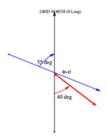
Figure 1: Geometry of measurements presented herein. $\phi$=0 corresponds to reference for primary reflection data. Surface iceflow direction at South Pole is shown in red, corresponding to $\phi$=–15 degrees ($\equiv$+165 degrees). Magnitude of iceflow is measured to be 10 m/yr, and uniform to a depth of $\sim$2 km. Measurements taken at South Pole in January, 2004, referred to later in this document, corresponded to an antenna alignment axis of $\sim$–11 degrees (+169 degrees).

II Set-up, Calibration, and in-air broadcasting

Two 1/2-inch thick jumper coaxial cables, each approximately 25 m long, were fed from the RICE experiment inside the Martin A. Pomerantz Observatory (MAPO) building at the South Pole through a conduit at the bottom of the building and out onto the snow. Each cable was then connected to a TEM horn antenna, manufactured by the Institute of Nuclear Research (INR), Moscow. These antennas were also used in our previous measurement of the ice attenuation length at the South Pole(Barwick and others,, 2005). As with our previous measurement, for in-ice transmission, each horn antenna is placed face-down on the surface looking into the snow. Signals are lowpass filtered, with a variety of filters, then high-pass filtered to remove components above 1 GHz, notch filtered to suppress the large South Pole background noise at 450 MHz which serves as the station Land Mobile Radio carrier, and finally amplified by +52 dB prior to data acquisition. The horn antennas have reasonably good transmission characteristics, from 60 MHz up to 1300 MHz, as indicated by the Voltage Standing Wave Ratio (VSWR) plots in Fig. 2.

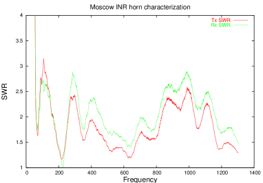
Figure 2: Voltage Standing Wave Ratio (VSWR) for horn antennas used in measurements described herein.

We note that, within 1–2 wavelengths, downward-facing horns see some mixture of air+snow, which down-shifts the antenna response in frequency by some 10-20%, and also narrows the beam pattern. The measured frequency response shown in Figure 2 is that of the horn antennas in their experimental configuration and therefore should correctly represent the horn characteristics relevant to this measurement. The forward gain of the horns is expected to be $\sim$10 dBi in air, or $\sim$12–15 dBi in-ice. In an attempt to minimize in-air ringing between the transmitter horn (Tx) and the receiver horn (Rx), the two antennas were placed on opposite sides of MAPO. For in-air broadcasting measurements made as a cross-check of polarization isolation, the horns were propped up onto the snow surface with their open ends facing each other on the same side of MAPO. In this case, the +52 dB amplifier was removed and signals were read directly at the digital oscilloscope.

Signals were taken from an AVIR-1C pulse generator into the transmitter horn; data acquisition of receiver horn waveforms was performed using the LeCroy 950 Waverunner digital oscilloscope. This scope features good bandwidth (1 GHz) and a high maximum digitization speed (16 GSa/sec). For the measurements described herein, the scope sampling rate was generally set to 2 GSa/sec. In order to enhance signal-to-noise, many waveforms (40,000 typically) were averaged. As waveform averaging requires a) stable scope capture trigger relative to b) the signal output, both a) and b) were taken directly from the AVIR-1C, as depicted in Figure 3.

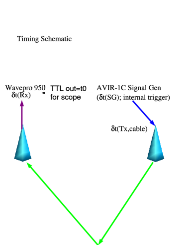
Figure 3: Trigger timing schematic for primary measurements described herein.

In order to correlate our observed internally-reflected signals with previous measurements, we must subtract off the time-delay due to cable propagation. We measure a cable propagation time delay of ($\delta t_{cable}$) $\approx$+190 ns (Figure 4) relative to the oscilloscope trigger time.

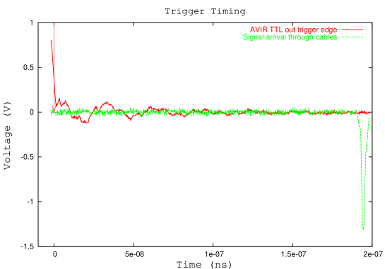
Figure 4: Oscilloscope trigger (falling edge on left) with respect to signal through cables (as in previous plot, with time scale and voltage units more explicit).

We have attempted to estimate the isolation between “Vpol” (along the long axis of the horns) and “Hpol” (the perpendicular axis) by broadcasting signals in-air, with both antennas on the same side of MAPO and facing each other on the snow. This measurement is complicated by the possibility of reflections off both the snow surface itself, as well as the aluminum side of the MAPO building. Although previous similar work at Taylor Dome indicates that the former reflection does not seem to produce substantially noticeable effects, the reflection off the metal sides of MAPO is likely to be non-negligible. Because of interference between the three possible routes (direct plus the two reflections mentioned above), we restrict our attention to the first few ns of received signal when broadcasting directly through air. In order to qualitatively assess interference effects at a particular separation distance, measurements were made at separation distances of 93 ft. and 83 ft., respectively. Antenna geometry is referenced relative to the side of the TEM horn where the cable is attached to the feed point; this side is defined as “+”. We define “+H” as the antenna orientation when the antenna is lying horizontally and the feed cable points directly away from MAPO; “+V” denotes the antenna orientation when the antenna is oriented vertically with the feed cable pointing away from the snow surface. Based on Figures 6 and 6, the estimated V:H power isolation, when the transmitter is broadcasting lying ’horizontally’ on the snow is approximately 5 dB. The signal duration is estimated to be of order 5–10 ns.

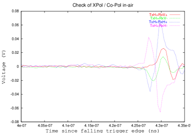
Figure 5: In-air broadcasts, 93 foot separation between transmitter and receiver; transmitter oriented horizontally in “H+” configuration.

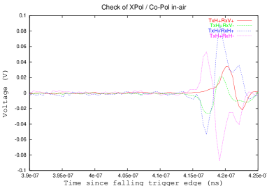
Figure 6: In-air broadcasts, 83 foot separation between transmitter and receiver; transmitter oriented horizontally in “H+” configuration.

When the transmitter is broadcasting in the “+V” configuration, the cross-talk is considerably smaller (Figure 7). Isolation of 5 dB should be adequate in our search for birefringent effects. Based on these Figures, we also estimate the total absolute gain uncertainty to be approximately a factor of two. Note that an antenna with an azimuthally-symmetric monopole beam pattern has no sensitivity to birefringence. In that case, any arbitrary signal has the same components along the ordinary and extraordinary axes.

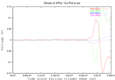
Figure 7: In-air broadcasts, 93 foot separation between transmitter and receiver; transmitter oriented horizontally in “V+” configuration.

III In-Ice broadcasting

Following the in-air measurements, the primary measurements of reflection returns when broadcasting through the ice were then conducted. Despite the shielding expected from the intervention of MAPO between transmitter and receiver, considerable through-air signal leakage between Tx and Rx is observed just after the trigger. This large background dominates our acquired waveforms for approximately 5 microseconds after the initial trigger, and prevents observation of in-ice reflections during that time period. In the absence of lowpass filtering, this large background will saturate the amplifier, resulting in an amplifier settling time which extends tens of microseconds. Most of this power, however, is broadcast at low frequencies and can be suppressed with appropriate filtering. Figure 8 shows sample waveforms acquired using different filters, beginning several microseconds after the initial trigger. In the absence of any filtering, no signals are clearly visible. Filtering out components below 200 MHz is sufficient to mitigate amplifier saturation effects. Our default configuration employs a Mini-Circuits model #NHP250 highpass filter, which provides $>$70 dB suppression below 200 MHz, followed by a logarithmic turn-on through the 200-250 MHz regime.

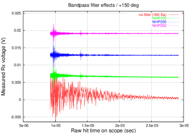
Figure 8: Comparison of received signals, for different filters applied to receiver output. We use, as a default, the NHP250 filter.

Figures 10 and 10 show the waveforms obtained for the time intervals corresponding to 9.2–14.2 and 14.2–29.2 microseconds after the scope trigger, for filtering with NHP250 vs. NHP200 filters. In detail, the latter still shows some indications of amplifier settling. The gross features of the two waveforms are observed to be comparable.

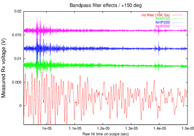
Figure 9: Filter comparison, zooming in on 5 microseconds of data between 9.2 and 14.2 $\mu$s after trigger.

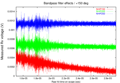
Figure 10: Filter comparison, zooming in on 15 microseconds of data between 14.2 and 29.2 microseconds after trigger.

With the NHP250 filter in place, measurements were made to sample the noise environment, in the absence of any transmitted signal. Figure 12 shows the acquired waveform.

Figure 11: Time-domain voltage profile, transmitter off.

Figure 12: Projection of previous plot onto voltage axis, showing Gaussian-like distribution expected for thermal noise.

Figure 12 shows the distribution of acquired voltages; we observe a roughly Gaussian distribution, as expected by thermal noise. The rms of this distribution is measured to be 35 microVolts. In the absence of any noise contributed by the digital oscilloscope itself, this voltage can be compared to the thermal noise voltage at T=223 K expected in a $\sim$750 MHz bandpass $B$ looking into an $R$=50 $\Omega$ load incoherently averaged over N=40000 samples: $V\sim\sqrt{kTBR/N}$. Taking into account the cable losses already shown, as well as the effect of the +52 dB amplifier and the filter, we obtain an estimate of approximately 30 microvolts, roughly consistent with observation.

In our initial configuration, both antennas were co-aligned with their long axis parallel to the MAPO building (this simply provided an easily reproducible $\phi$=0 azimuthal reference and is identical to the $\phi$=0 line shown in Figure 1.). Figure 13 shows that: a) waveforms are reproducible from one 40K average to the next, and b) after moving the antennas around for one day, and then replacing them at their original location, waveforms are also reproducible.

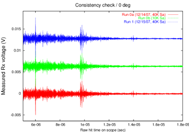
Figure 13: Check of consistency between measured waveforms, all taken in $\phi$=0 orientation.

We attempted to detect birefringent effects using the same approach as that used in our previous analysis(Besson and others,, 2008), namely, we search for a measurable time difference in received signals, as a function of the orientation of the long axis (transmitted signal polarization axis) of the TEM horns. Our initial hope was to be able to detect the reflection off of the bedrock, some 2.8 km below the surface. Due to the relative weakness of our signal generator, however, as well as the large absorption expected in the warmer ice near the bedrock, no clear signal is observed in the time delay region around 33 microseconds, as expected for a bottom reflection (Fig. 14). A follow-up measurement will employ a signal generator with a roughly order-of-magnitude higher voltage output.

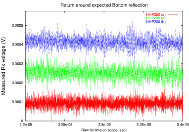
Figure 14: Return signal in time interval expected to bracket bedrock reflection signal.

Since the bottom reflection was too weak to be observable, internal layers were used as scattering planes. We co-rotated the horns in the positive $\phi$ direction, and took measurements every 30 degrees. In addition, data were taken in 3 different “cross-polarization” configurations, designated by a Tx orientation and an Rx orientation. Figure 16 shows the signals received over the time interval from 5–25 microseconds after the initial trigger.

As a check that the general features are relatively insensitive to the exact placement of the antennas, data were also taken with the transmitter horn and receiver horn both displaced approximately 10 meters in the +90 degree direction (Figure 16), and with a slightly different trigger (and also trigger delay) configuration.

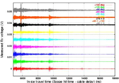
Figure 15: 5–25 microsecond waveform captures, after averaging, for various azimuthal angles. Data configuration corresponds to default for most of measurements cited in this paper.

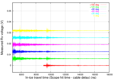
Figure 16: 5–25 microsecond waveform captures, after averaging, for various azimuthal angles. Antennas have been translated along y-axis (orthogonal to MAPO), but orientation angles are preserved.

The general signal features look very similar in the displaced configuration as the original configuration.

The first clear return is observed at a time delay of approximately 6 microseconds after the trigger time. Knowing the index-of-refraction profile at South Pole, we convert this to return signal vs. depth (Figure 17).

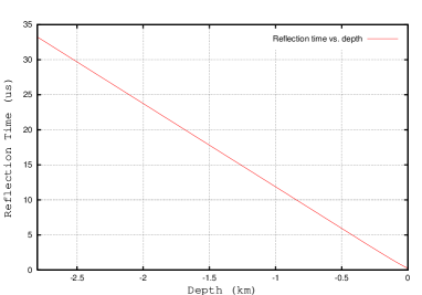
Figure 17: Expected reflection return time, as a function of depth of reflecting layer.

We observe a small, apparently monotonic variation in the received signal phase with $\phi$ (Figure 19). Note that a value of 0.12% birefringence, as measured in our Taylor Dome analysis, would imply a shift of amplitude $\sim$4 ns between Tx/Rx alignment with the ordinary vs. extraordinary optical axes. The observed maximum time shift ($\sim$2 ns) implies a birefringent asymmetry of $<$0.05%. We cannot exclude the possibility that some of the observed phase shifts are the result of interference effects between signals with arrival times coincident within $\sim$2 ns.

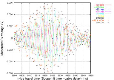
Figure 18: Overlay of signal reflections around t=6 microseconds after trigger.

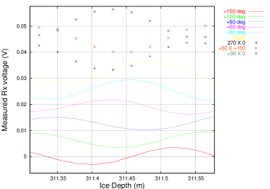
Figure 19: Zoom of previous figure, showing monotonic variation in phase as a function of orientation angle.

We also observe a considerable anisotropy in the received signal amplitude, which also varies sinusoidally. This could be explained as the result of a polarization-dependent reflection coefficient. It might also be explained as the result of polarization-dependent absorption.

Our resolution on birefringent effects obviously increases with the depth of the layer probed. Starting with Figure 16, we see clear subsequent structure at time delays of 9.6, 13.9, 17.2, and 19.6 microseconds, as zoomed in Figures 21, 21,

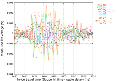
Figure 20: Ensemble of observed reflections in time interval around 9.6 microseconds after trigger.

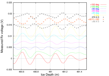
Figure 21: Zoom of observed reflections in time interval around 9.6 microseconds after trigger.

22,

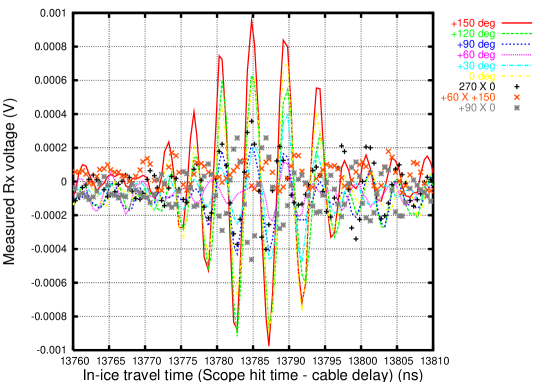
Figure 22: Overlay of 13.9 microsecond reflections, as a function of orientation angle, default geometry and trigger configuration.

23 (slightly different geometry)

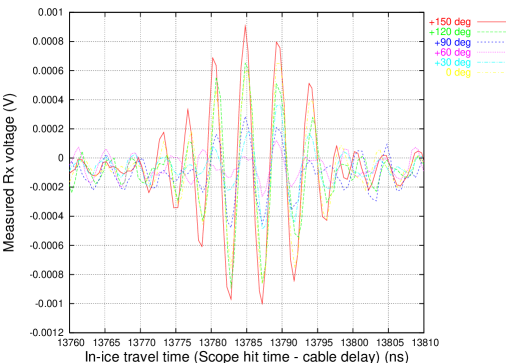
Figure 23: Similar to previous plot, but made with antennas translated on the snow surface, and with a slightly different trigger configuration.

24,

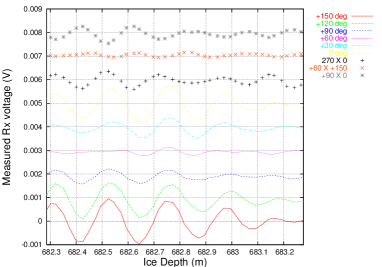
Figure 24: Zoom of 13.9 microsecond reflections, default configuration.

25

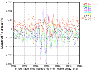
Figure 25: Ensemble of reflections observed in time interval around 17.2 microseconds after trigger.

and 26.

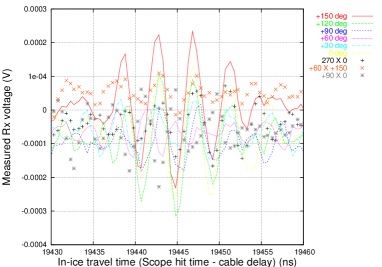
Figure 26: Ensemble of reflections observed in time interval around 19.6 microseconds after trigger.

We select the 13.9 microsecond delayed signals as those with sufficient signal-to-noise, yet with a longer delay than the Taylor Dome results as our primary dataset. We note in Figure 22 that the observed waveforms are very consistent with each other in both shape and arrival time. Assuming that we are sensitive to shifts of order $\pi/2$ (i.e., $\approx$1 ns), this puts a limit on the birefringent asymmetry at South Pole to be $<$0.01%. As a check of this conclusion, we have compared the signals observed in the primary data-taking configuration with signals observed with displaced antennas and slightly different trigger (Figure 23). The secondary data configuration gives results consistent with the primary data configuration.

The 19.6 microsecond data has the largest time delay of our observed signals. Although there is an apparent shift of a few ns between the +150 degree and +60 degree peaks, the relatively larger noise contribution to the latter waveform renders this comparison somewhat inconclusive. All other time delays, relative to the +150 degree data, are consistent with zero, and consistent with the interpretation of no clearly observable birefringent effects.

III.1 Comment on Reflected Signal Strength

For coherent scattering, the strength of any reflected signal is expected to follow the radar equation for the received power $P_{Rx}=P_{Tx}{\tt R}G_{Tx}G_{Rx}e^{-r/L_{atten}}/(4\pi r^{2})$, with $G_{Tx}$ and $G_{Rx}$ the forward gain of transmitter and receiver in-ice, $r$ the total transit distance (i.e., twice the depth), $L_{atten}$ the power attenuation length over the frequency range of interest, and ${\tt R}$ the power reflection coefficient. Alternately, $G_{Rx}$ is often equated to the radar cross-section $\sigma$ times the effective area $A_{eff}$ of the receiving antenna. We estimate this product to be equal to 0.5 m x 0.5 m, and $\sigma\sim 4\pi~{}m^{2}$. Given a value of $L_{atten}$, one can therefore estimate the reflection coefficient based on the measured power. In practice, the uncertainty on the attenuation length is sufficiently large that this error dominates any estimate of ${\tt R}$. As expected, the most prominent reflections are those due to the closest layers, corresponding to the most shallow returns. As before, we do observe a large variation in the amplitude of the return signal for the 13.9 us reflected signal (“$A_{13.9}$), however (Table 2). We also observe considerable power evidently transferred from the co-pol to the cross-pol orientation. This will require more detailed investigation in the future in order to assess the possible impact on neutrino detection efforts.

Orientation	$|V_{max}|$ (mV)
+180 deg	0.897
+150 deg	0.975
+120 deg	0.917
+90 deg	0.429
+60 deg	0.235
+30 deg	0.477
0 deg	0.881

Table 2: Peak voltages for 13.9 us reflection signal, as a function of angle. Note the $2\pi$ periodicity in the signal amplitude. Direct application of the radar equation, using values of attenuation length of order 1 km, indicates that the reflection coefficient is less than -22 dB. We note that the maximum amplitude signal aligns with the local global ice flow direction to within $\sim$15 degrees.

We have checked the uniformity of the observed reflection return waveforms, as shown in Fig. 27. For this Figure, signals have been scaled by the appropriate scale factor needed to match the peak voltage to that observed at $t\sim 6\mu$s. If the reflection coefficients were uniform, we would expect the ratios of ($A_{9.2}/A_{6})/(A_{13.9}/A_{9.2}$) to be approximately 1. Instead, we observe a ratio of ratios somewhat less than 1, indicating non-uniformity of the reflection coefficients at the internal scattering layers.

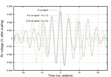
Figure 27: Comparison of shape of 6 microsecond, 9.2 microsecond, and 13.9 microsecond reflections.

In the frequency domain, the observed reflected signal retains most of the initially broadcast signal in the frequency regime above the highpass filter (Figure 28). Assuming that the reflection coefficient is frequency-independent, this is qualitatively consistent with our earlier study, which indicated only slight dependence of attenuation length with frequency.

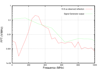
Figure 28: FFT of initially broadcast signal vs. FFT of signal measured in receiver horn.

IV Investigation of Faraday Rotation

Three obvious factors can, in principle, be responsible for the observed cross-polarized signal strength. These factors, which have different time dependences, are: a) cross-talk between the H and V polarization response of the antenna (time-independent), b) layer-specific reflection characteristics (specific at the time of a given reflection), and c) Faraday rotation, essentially equivalent to birefringence of circularly polarized waves. (proportional to pathlength). Note that, since a given material experiences a positive(/negative) phase rotation when the ${\hat{k}}$-vector is parallel(/anti-parallel) to the applied magnetic field, the phase rotation is (in general) not canceled over a round-trip path. (This conclusion is not changed if one assumes an inversion of the wave when reflected off a higher index-of-refraction medium.) In general, although birefringent effects will project onto ordinary and extra-ordinary axes, it will not result in a cross-polarized signal, although the received signal strength will be modulated due to interference effects, if the receiver time resolution is sufficiently coarse.

For a given material in a magnetic field $B$, the phase advance $\theta$ due to Faraday rotation through a pathlength $l$ is expressed in terms of the Verdet constant as: $\theta=VlB$. For a given material, the Verdet constant can be expressed in terms of the Bohr magneton as $V=\lambda dn/d\lambda$, with $n$ the index-of-refraction of the material. Using $dn/d\lambda\sim 10^{-4}$ over the wavelength interval of interest(Warren,, 1984), we obtain (mks units), $V$=0.02 rad/(m-T) at 300 MHz, in which case this is unlikely to be a significant effect.

Due to its dependence on pathlength, Faraday rotation can therefore be directly probed by plotting the ratio of the cross-polarized amplitude to the co-polarized amplitude as a function of time delay. Although the phase of the cross-polarized signal observed reflecting off discrete internal layers shows no obvious pattern (e.g., the 13.9 microsecond (/17.2 microsecond) +90 degree co-polarized reflected signal is in phase (/out of phase) with the cross-polarized signal), the ratio of amplitudes (Figure 29) indicates a suggestive modulation with period $\sim$8 microseconds. Interpreted as pure Faraday rotation, this would indicate a $\sim\pi$ polarization axis rotation for each 800 m of traversed ice depth.

Figure 29: Ratio of co-polarized to cross-polarized signal amplitude, as a function of time delay. Random thermal noise should average to zero on this plot; Faraday rotation would result in a modulated signal with time delay.

As a cross-check of the apparently large power being fed from one polarization into the cross-polarization, we also attempted to broadcast using a long dipole transmitter instead of the horn Tx, aligned along two orthogonal axes (corresponding to zero and 90 degrees, respectively). Given the lower forward gain of the dipoles, and the poorer frequency-response matching, we observe only the return at $\sim 6\mu$s, with approximately equal amplitude (Figure 30) in co-pol vs. cross-pol orientations.

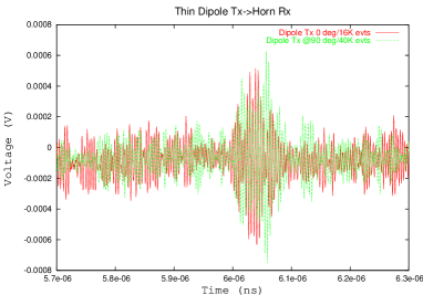
Figure 30: Signals observed using a long-dipole as transmitter antenna.

V Comparison with previous data

Figure 32 shows the co-polarized vs. cross-polarized data taken previously, in January 2004(Barwick and others,, 2005). Although not noted at the time, the clear presence of the scattering layer around 14 $\mu$s is evident from the Figures, as well as the presence of large amplitude signals in the cross-polarization configuration, not necessarily present in the co-polarization configuration. The horn orientation is approximately 160 degrees, in the coordinate system used for our current measurement.

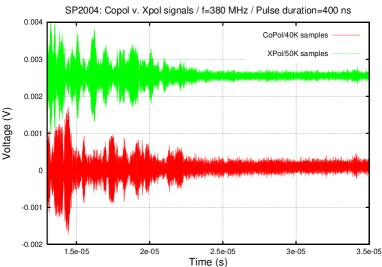
Figure 31: Cross- vs. copolarized signals observed in previous study, 400 ns signal duration.

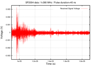
Figure 32: Copol signals observed in previous study, 40 ns signal duration.

We note that, in our previous study conducted at Taylor Dome, although direct evidence was observed for birefringence in scattering of radio waves off the bedrock, no clear returns from internal layers, prior to the bedrock reflection, were evident.

Using publicly available data from the CRESIS group, based at the University of Kansas, we have also attempted to extract evidence for birefringent effects based on their Greenland ice thickness aerial survey data. Since the CRESIS data includes the aerial velocity vector as data are taken, we have searched for a statistical separation between the depth recorded when the plane is flying parallel to the known ice-flow direction (taken from (Rignot and Kanagaratnam,, 2006)) vs. perpendicular to the known ice-flow direction. Figure 33 shows the results of this study. The rms of these distributions ($\sim$10 m, or $\sim$100 ns in total in-ice travel time) is insufficient to discern clear evidence for the sought-after birefringent asymmetry.

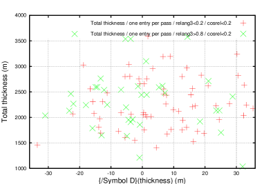
Figure 33: Depth difference recorded by CRESIS data, at a given point on the Greenland continent. Green corresponds to difference in recorded depths for cases where plane is flying perpendicular to known ice-flow direction vs. parallel to known ice-flow direction; red corresponds to (parallel-perpendicular) case. Birefringence would result in a difference in the centroid of the red vs. green points.

VI Summary

There has been increasing attention given to birefringence as responsible for radio-frequency interference effects observed in Antarctic ice. Having made a similar measurement at Taylor Dome, our goal in this analysis was to directly measure birefringence, as indicated by a time-delay between reflected signals received along two orthogonal azimuthal polarizations. For the purposes of this study, internal scattering layers were used as reflecting planes, which offered the possibility of correlating time-delays between successive reflecting planes with the crystal orientation in those intermediate layers. No obvious evidence for birefringence is observed. If true, this conclusion supports the suitability of the South Pole as a radio-based neutrino detection site, compared to other locales across the Antarctic continent, where birefringent effects have been claimed. We do observe a variation in scattered signal, as a function of azimuth, as previously detected in a similar, albeit frequency-based, measurement. Our results, however, disfavor that amplitude variation as a birefringent-related effect, and may require further investigation of the chemical and electrical properties of internal scattering layers. There is, in fact, some data available on dust layers at the South Pole(Bramall and others,, 2005), however we have not made a conclusive correlation between layering observed in this study and layers observed in previous studies.

VII Acknowledgments

This work is supported by the NSF through grant OPP-0338219. The author particularly thanks Chris Allen (U. of Kansas), Prasad Gogineni (U. of Kansas), Steve Barwick (U. of California, Irvine), Kenichi Matsuoka (U. of Washington), and Jiwoo Nam (National Taiwan University, Taiwan) for very helpful discussions.

References

- Abassi and others, (2007) R. Abassi and 253 others (the IceCube Collaboration), “Contributions to The 10th International Conference on Topics in Astroparticle and Underground Physics (TAUP) 2007, Sendai, Japan”, arXiv:0712.3524 (2007).
- Barwick and others, (2005) S. Barwick, D. Besson, P. Gorham, D. Saltzberg, “South Polar in situ Radio Frequency Ice Attenuation”, J. Glac. 04J067 (2005).
- Barwick and others, (2006) S. W. Barwick and 40 others, “ Constraints on Cosmic Neutrino Fluxes from the ANITA Experiment”, Phys. Rev. Lett. 96, 171101 (2006).
- Besson, (2006) D. Besson, “ Radiowave Neutrino Detection”, arXiv:astro-ph/0611365, accepted for publication in Nucl. Instr. Meth. A 48086 (2008).
- Besson and others, (2008) D. Besson, J. Jenkins, S. Matsuno, J. Nam, M. Smith, “ In situ radioglaciological measurements near Taylor Dome, Antarctica and implications for UHE neutrino astronomy”, arXiv:astro-ph/0703413, accepted by Astropart. Phys. (2008).
- Bramall and others, (2005) N. E. Bramall, R. C. Bay, K. Woschnagg, R. A. Rhode, P. B. Price, “A deep high-resolution optical log of dust, ash, and stratigraphy in South Pole glacial ice”, Geo. Res. Lett. 32, 21815 (2005).
- CRESIS, (2008) (CRESIS) https://www.cresis.ku.edu/research/dataproductsandmodeling.html (2008).
- Doake and others, (2002) C. Doake, H. Corr, A. Jenkins, “Polarization of radio waves transmitted through. Antarctic ice shelves”, Ann. Glac. 34 (1), 165-170 (2002).
- Doake and others, (2003) C. Doake, H. Corr, A. Jenkins, K. Nichols, C. Stewart, “Applications of SAR Polarimetry and Polarimetric Interferometry”, Euro. Space Agency pub. 529, 313-320, (2003).
- Hargreaves, (1977) N. D. Hargreaves, “he polarization of radio signals in the radio echo sounding of ice sheets”, J. Phys. D: Applied Physics 10(9), 1285-1304 (1977).
- Hargreaves, (1978) N. D. Hargreaves, “The radio frequency birefringence of polar ice”, J. Glac. 21, 301-313 (1978).
- Kravchenko and others, (2005) I. Kravchenko, D. Besson and J. Meyers, “In situ index of refraction measurements of the South Polar firn with the RICE detector”, J. Glac. 03J061 (2005).
- Kravchenko and others, (2007) I. Kravchenko and 14 others, “ Event Reconstruction and Data Acquisition for the RICE Experiment at the South Pole”, arXiv:0705.4491, in preparation for submission to Phys. Rev. D (2007).
- Matsuoka and others, (2003) K. Matsuoka, T. Furukawa, S. Fujita, N. Maeno N, S. Uratsuka, R. Naruse, O. Watanabe, “Crystal orientation fabrics within the Antarctic ice sheet revealed by a multipolarization plane and dual-frequency radar survey”, J. Geophys. Res. 108 (B10) (2003).
- Matsuoka and others, (2004) K. Matsuoka, S. Uratsuka, S. Fujita, F. Nishio, ”Ice-flow-induced scattering zone within the Antarctic ice sheet revealed by high-frequency airborne radar”,J. Glac. 50(170), 382-388 (2004).
- SOARa, (2008) (SOARa) http://www.ig.utexas.edu/research/projects/soar/ (2008).
- SOARb, (2008) (SOARb) http://www.ig.utexas.edu/research/projects/soar/data/PPT/SOAR_ppt.htm (2008).
- Price and others, (2002) P. B. Price and 9 others, “Temperature profile for glacial ice at the South Pole: Implications for life in a nearby subglacial lake”, PNAS 99, 12, 7844 (2002).
- Rignot and Kanagaratnam, (2006) Rignot and Kanagaratnam, “Changes in the Velocity Structure of the Greenland Ice Sheet”, Science, 311, 5763, 986 (2006).
- Warren, (1984) ”Optical constants of ice from the ultraviolet to the microwave”, Appl. Opt. 23, 8, 1206 (1984).