On approximating the distributions
of goodness-of-fit test statistics
based on the empirical distribution function:
The case of unknown parameters

Abstract

This paper discusses some problems possibly arising when approximating via Monte-Carlo simulations the distributions of goodness-of-fit test statistics based on the empirical distribution function. We argue that failing to re-estimate unknown parameters on each simulated Monte-Carlo sample – and thus avoiding to employ this information to build the test statistic – may lead to wrong, overly-conservative testing. Furthermore, we present a simple example suggesting that the impact of this possible mistake may turn out to be dramatic and does not vanish as the sample size increases.

I Introduction

This paper discusses some problems possibly arising when approximating – via Monte-Carlo simulations – the distributions and critical values of the most commonly employed goodness-of-fit (GoF) tests based on empirical distribution function (EDF) statistics D’Agostino and Stephens (1986); Thode (2002).

This situation arises very frequently – in many areas of statistical physics or econophysics – when the researcher aims at fitting some experimental or empirical (univariate) sample with a parametric (univariate) probability distribution whose parameters are unknown. In such cases, the goodness of fit may be ex-post evaluated by employing standard statistical tests based on the EDF. If, as typically happens, critical-value tables are not available, one has to resort to Monte-Carlo methods to derive the approximated distribution of the test statistics under analysis.

We show that, when testing with unknown parameters, critical values (and consequently testing outcomes) may be dramatically sensible to the details of the Monte-Carlo procedure actually employed to approximate them. More specifically, we argue that the researcher may sometimes build inaccurate critical-value tables because he/she fails to perform a crucial step in his/her Monte-Carlo simulation exercises, namely maximum-likelihood (ML) re-estimation of unknown parameters on each simulated sample. In our opinion, this is a lesson worth learning because critical-value tables are only available for particular distributions (e.g., normal, exponential, etc.). In all other cases, our study indicates that failing to correctly specify the Monte-Carlo approximation procedure may lead to overly-conservative hypothesis tests.

The rest of this paper is organized as follows. Section 2 formalizes the general GoF test under study and discusses the main problems associated to the approximation of EDF-based GoF test-statistic distributions from a theoretical perspective. Section 3 presents an application to the case of normality with unknown parameters. Finally, Section 4 concludes with a few remarks.

II Approximating EDF-based GoF test-statistic distributions

In many applied contexts, the researcher faces the problem of assessing whether an empirical univariate sample $\underline{x}_{N}=(x_{1},\dots,x_{N})$ comes from a (continuous) distribution $F(x;\theta)$, where $\theta$ is a vector of unknown parameters. EDF-based GoF tests D’Agostino and Stephens (1986); Thode (2002) employ statistics that are non- decreasing functions of some distance between the theoretical distribution under the null hypothesis $H_{0}:\underline{x}_{N}\sim F(x;\theta)$ and the empirical distribution function constructed from $\underline{x}_{N}$, provided that some estimate of the unknown parameters is given.

In what follows, we will begin by focusing on the simplest case where $F(x;\theta)$ has only location and scale unknown parameters (we will discuss below what happens if this is not the case). Furthermore, we will limit the analysis to four out of the most used EDF test statistics, namely Kolmogorov-Smirnov Massey (1951); Owen (1962), Kuiper Kuiper (1962), Cramér - Von Mises Pearson and Stephens (1962) and Quadratic Anderson- Darling Anderson and Darling (1954), with small-sample modifications usually considered in the literature .

It is well-known that if one replaces $\theta$ with its maximum likelihood (ML) empirical-sample estimate $\hat{\theta}(\underline{x}_{N})$, the distributions of the EDF test statistic under study can be shown to be independent on the unknown true parameter values David and Johnson (1948). However, test-statistic distributions are hard to derive analytically. They must be therefore simulated via Monte-Carlo and critical values must be accordingly computed. To do so, let us consider a first possible procedure:

Procedure A

Step A1

Generate, by means of standard simulation techniques Devroye (1986), a sufficiently large number (say, $M>>0$) of independently-drawn N-sized samples $\underline{z}_{N}^{j}=(z_{1}^{j},\dots,z_{N}^{j})$, $j=1,\dots,M$, where each $z_{i}^{j}$ is an i.i.d. observation from a $F(x;\hat{\theta}(\underline{x}_{N}))$, i.e. from the distribution under $H_{0}$ where unknown parameters are replaced by their empirical-sample estimates;

Step A2

For each N-sized sample $\underline{z}_{N}^{j}$, compute an observation of the EDF test statistic under study by comparing the EDF constructed from $\underline{z}_{N}^{j}$ with the theoretical distribution
$F(\underline{z}_{N}^{j},\hat{\theta}(\underline{x}_{N}))$, i.e. when $F$ is computed at the empirical sample observations and unknown parameters are always replaced with estimates $\hat{\theta}(\underline{x}_{N})$ obtained once and for all from the empirical sample;

Step A3

Once Step A2 has been carried out for all $M$ samples, compute the empirical distribution function $T$ of the test statistic;

Step A4

Compute (upper-tailed) critical values, for any given significance level $\alpha$, by employing the empirical distribution function $T$ of the EDF test statistic as obtained in Step A3.

At a first scrutiny, the above procedure seems to be correct. Indeed, the procedure tells us to approximate the distribution of the test statistic under study by repeatedly compute it on a sufficiently large number of i.i.d. samples, all distributed as if they came from the null distribution $F(\cdot,\theta)$, when the unknown parameters are replaced with their empirical sample estimate $\hat{\theta}(\underline{x}_{N})$.

Despite its appeal, however, Procedure A can be shown to be wrong, in the sense that it generates a completely wrong approximation to the “true” distribution of the test statistic under the null hypothesis.

The reason why Procedure A is not correct lies in Step A2. More precisely, when we compare the EDF constructed from $\underline{z}_{N}^{j}$ with the theoretical distribution $F(\underline{z}_{N}^{j},\hat{\theta}(\underline{x}_{N}))$, we are assuming that our estimate for $\theta$ does not depend on the actual sample $\underline{z}_{N}^{j}$ under analysis. This is the same as presuming that the hypothesis test is performed for known parameters. On the contrary, sticking to the null hypothesis implies that the theoretical distribution which should be compared to the EDF of $\underline{z}_{N}^{j}$ must have parameter estimates that depend on the actual Monte-Carlo sample $\underline{z}_{N}^{j}$. In other words, scale and location parameters $\theta$ must be re-estimated (via, e.g., ML) each time we draw the Monte-Carlo sample. Let $\hat{\theta}(\underline{z}_{N}^{j})$ be such estimate for sample $j$. This means that the theoretical distribution to be used to compute the test statistic would be $F(\underline{z}_{N}^{j},\hat{\theta}(\underline{z}_{N}^{j}))$ and not $F(\underline{z}_{N}^{j},\hat{\theta}(\underline{x}_{N}))$. The correct procedure therefore reads:

Procedure B

Step B1

Same as A1;

Step B2

For each N-sized sample $\underline{z}_{N}^{j}$, compute an observation of the EDF test statistic under study by comparing the EDF constructed from $\underline{z}_{N}^{j}$ with the theoretical distribution $F(\underline{z}_{N}^{j},\hat{\theta}(\underline{z}_{N}^{j}))$, i.e. when $F$ is computed at the empirical sample observations and unknown parameters are replaced with estimates $\hat{\theta}(\underline{z}_{N}^{j})$ obtained from the j-th Monte-Carlo sample;

Step B3

Same as A3;

Step B4

Same as A4.

How dramatic is the error we make in applying Procedure A instead of Procedure B? Do we get a more conservative or less conservative test by using the wrong procedure? In other words, can we detect significant shifts in the Monte-Carlo approximation to the distribution of the test statistics under study when we compare Procedures A and B? In the next section, we will answer these questions by providing a simple example.

III Application: Testing for Normality with Unknown Parameters

Let us consider the null hypothesis that the empirical sample comes from a normal distribution $N(\mu,\sigma)$ with unknown mean ($\mu$) and standard deviation ($\sigma$). In such a case, parameters may be replaced by their ML estimates $(m(\underline{x}_{N}),s(\underline{x}_{N}))$, i.e. sample mean and standard deviation. In this case critical values for the four test statistics under study are already available. Our goal, for the sake of exposition, is therefore to compare Monte-Carlo approximations to the distributions of the four test statistics obtained under Procedures A and B.

We thus have two setups. In the first one (Procedure A), one does not re-estimate the parameters and always employs $(m(\underline{x}_{N}),s(\underline{x}_{N}))$ to build the theoretical distribution. In the second one (Procedure B), one re-estimates via ML mean and standard deviation on each simulated sample by computing $(m(\underline{z}_{N}^{j}),s(\underline{z}_{N}^{j}))$ and then uses them to approximate the theoretical distribution of the test statistic.

Our simulation strategy is very simple. Since the argument put forth above does not depend on the observed sample’s mean and standard deviation, we can suppose that $(m(\underline{x}_{N}),s(\underline{x}_{N}))=(0,1)$ without loss of generality. For each of the four test statistics considered, we run Monte-Carlo simulations to proxy its distribution under the two setups above. In both setups, we end up with an approximation to the distribution of the four tests, from which one can compute critical values associated to any significance level (or p-value).

To begin with, Table 1 shows critical values for all 4 tests at $\alpha=0.05$ significance level, and for different combinations of $N$ (sample size) and $M$ (Monte-Carlo replications). It is easy to see that if we employ Procedure B, we obtain the same critical values published in the relevant literature for the case of normality with unknown parameters (compare, e.g., our table 1 with table 1A-1.3 at page 732 in Stephens, 1974). On the contrary, if we employ procedure A, critical values dramatically increase. The effect is of course more evident in the case of so-called “quadratic statistics” (Cramér-Von Mises and Quadratic Anderson-Darling), but is equally relevant also in the case of “supremum statistics” (Kolmogorov-Smirnov and Kuiper). What is more, Procedure A allows us to obtain critical-value figures which are very similar to those found in the literature for the case of normality with completely specified, known, parameters.

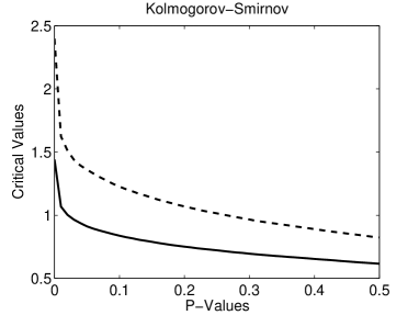
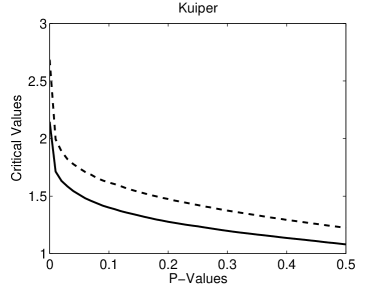
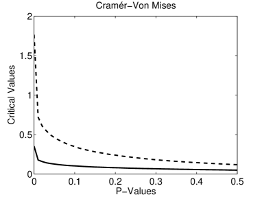
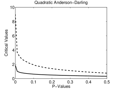
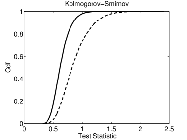
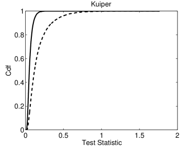
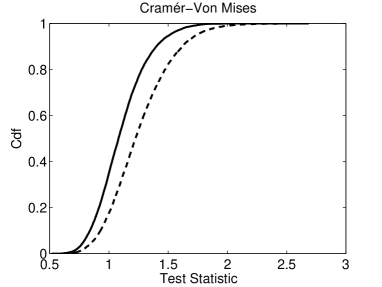
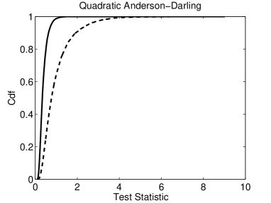
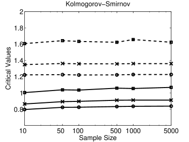
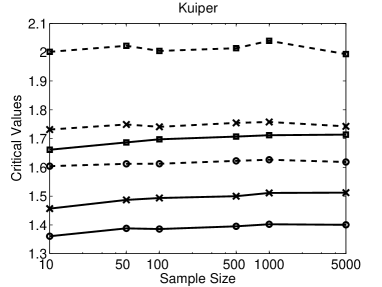
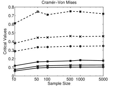
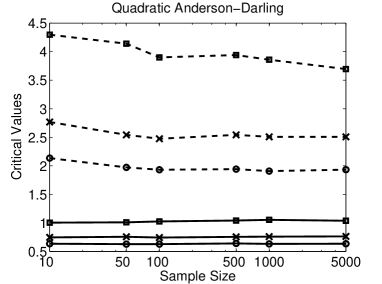
Table 1 also indicates that if we wrongly employ Procedure A, we end up with test statistics that are dramatically more conservative (at $\alpha=0.05$) than if we correctly employ Procedure B. This is true irrespective of the significance level. As Figure 1 shows, the A vs. B gap between critical values remains relevant for all (reasonable) p-value levels. In other words, the wrong choice of employing Procedure A induces a rightward shift of (and reshapes) the entire test-statistic distribution. To see this, in Figure 2 we plot the estimated cumulative distribution of all 4 test statistics under the two setups. Choosing Procedure A makes all tests much more conservative.

Finally, it is worth noting that the above results do not depend on the empirical sample size. In fact, one might argue that the mismatch between the two procedures may be relevant only for small $N$’s but should vanish as $N$ gets large. This is not true: the gap remains there as $N$ increases within an empirically-reasonable range and for any sufficiently large number of Monte-Carlo replications ($M$) – see Figure 3 for the case $M=10000$.

IV Concluding Remarks

In this paper, we have argued that failing to re-estimate unknown parameters on each simulated Monte-Carlo sample (and not employing this information to compute the theoretical distribution to be compared with the sample EDF) may lead to wrong, overly-conservative approximations to the distributions of GoF test statistics based on the EDF. Furthermore, as our simple application shows, the impact of this possible mistake may turn out to be dramatic and does not vanish as the sample size increases.

Notice that similar issues have already been discussed in the relevant literature Lilliefors (1967); Dyer (1974); Stephens (1974); Green and Hegazy (1976). More specifically, Stephens (1976) shows that the mean of the Anderson-Darling statistic shifts leftwards when the parameters of the population distribution are unknown. Furthermore, Stute (1993); Rao (2004) discuss the problem of approximating EDF test statistics from a rather theoretical perspective. Yet, despite the success of EDF-based GoF tests, no clear indications were given – to the best of our knowledge – about the practical correct Monte-Carlo procedure to be followed in order to approximate test-statistic distributions in the case of unknown parameters. This paper aims at shedding more light on the risks ensuing a wrong specification of the Monte-Carlo simulation strategy, in all cases where critical-value tables are not already available. Given the lack of contributions addressing this topic, and the subtle nature of the choice between Procedure A and B, our feeling is that mistakes may be more likely than it may seem.

A final remark is in order. In our discussion we deliberately focused only on the case where parameters to be estimated are location and scale. In such an “ideal” situation, as we noted, the distributions of the four EDF-based test-statistics that we have considered do not depend on the true unknown parameters. Therefore, in principle, to approximate their distributions one may generate, in Step B1, a sufficiently large number of independently-drawn N-sized samples from a $F(x;\theta^{\ast})$, where $\theta^{\ast}$ is any given value of the unknown parameters, and not necessarily their empirical-sample estimates $\hat{\theta}(\underline{x}_{N})$. Since the distribution of the test is location- and scale-invariant, we just need to make sure to apply Step B2 (i.e. re-estimation of $\theta$ using $\underline{z}_{N}^{j}$) in order to avoid the implicit assumption that parameters are known.

What happens if instead parameters are not location and scale but are still unknown? In such a case, very common indeed (e.g., when $F$ is a Beta or a Gamma distribution), test-statistic distributions do depend on the true unknown parameter values Darling (1955); Durbin (1975). Therefore, Step B1 may be considered as a first (good) guess towards the approximation of test-statistic distributions. In fact, when parameters are not location and scale, one cannot employ any given $\theta^{\ast}$ to generate Monte Carlo samples. Since the “true” test-statistic distribution depends on the “true” unknown parameter values, one would like to approximate it with a sufficiently similar (although not exactly equal) distribution, which can be easily obtained – provided that Procedure B is carried out – by employing the empirical sample estimates $\hat{\theta}(\underline{x}_{N})$. In such a situation, critical value tables are not typically available, because they would depend on the empirical sample to be tested. Monte-Carlo simulations are therefore required and choosing the correct Procedure (B) instead of the wrong one (A) becomes even more crucial than in the location - scale case.

Acknowledgments

This article enormously benefitted from comments and suggestions made by Richard Lockhart, who patiently went through the main points with his illuminating explanations. Thanks also to Michael Stephens and Fabio Clementi for their very useful remarks and suggestions. Any remaining errors are the sole responsibility of the authors.

		KS		KUI		CVM		AD2
N	M	Proc B	Proc A	Proc B	Proc A	Proc B	Proc A	Proc B	Proc A
	100	0.8220	1.2252	1.4235	1.6138	0.0690	0.2807	0.7194	2.2727
10	1000	0.8564	1.3035	1.4485	1.7270	0.0706	0.3707	0.6996	2.6139
	10000	0.8648	1.3482	1.4565	1.7314	0.0757	0.3800	0.7442	2.7667
	100	0.8159	1.4965	1.4376	1.7671	0.0985	0.5941	0.6863	3.1936
50	1000	0.8928	1.3813	1.4783	1.7715	0.1111	0.4512	0.7424	2.4106
	10000	0.8931	1.3623	1.4867	1.7489	0.1146	0.4446	0.7553	2.5414
	100	0.9380	1.4601	1.5831	1.7954	0.1308	0.4902	0.7664	2.7079
100	1000	0.8839	1.3525	1.5083	1.7162	0.1129	0.4634	0.7172	2.6332
	10000	0.8969	1.3587	1.4933	1.7407	0.1199	0.4478	0.7425	2.4740
	100	0.9177	1.2389	1.531	1.7857	0.1146	0.3455	0.7231	2.0889
500	1000	0.9125	1.3316	1.5139	1.7250	0.1273	0.4333	0.7769	2.3941
	10000	0.9108	1.3576	1.4998	1.7544	0.1261	0.4628	0.7543	2.5423
	100	0.9443	1.3723	1.4753	1.7879	0.1312	0.4116	0.7998	2.3795
1000	1000	0.9041	1.3858	1.5103	1.7814	0.1246	0.4674	0.7700	2.5817
	10000	0.9121	1.3606	1.5108	1.7575	0.1267	0.4578	0.7581	2.5076
	100	0.9689	1.2911	1.5656	1.8264	0.1405	0.4107	0.8099	2.2523
5000	1000	0.8944	1.3807	1.4801	1.7478	0.1204	0.4513	0.7180	2.4596
	10000	0.9116	1.3606	1.5120	1.7424	0.1274	0.4617	0.7613	2.5073

Table 1: Critical values at significance level $\alpha=0.05$ for the four EDF tests considered. Proc A: Always using empirical-sample estimates. Proc B: Parameters are re-estimated each time on Monte-Carlo sample. KS=Kolmogorov-Smirnov; KUI=Kuiper; CVM=Cramér-Von Mises; AD2=Quadratic Anderson-Darling.

Figure 1: Critical values versus P-values for the four test statistics under study. Empirical sample size: $N=5000$. Number of Monte-Carlo replications: $M=10000$. Solid line: Procedure B (parameters are re-estimated each time on Monte-Carlo sample). Dashed line: Procedure A (always using empirical-sample estimates).

Figure 2: Estimates of cumulative distribution function (Cdf) for the four test statistics under study. Empirical sample size: $N=5000$. Number of Monte-Carlo replications: $M=10000$. Solid line: Procedure B (parameters are re-estimated each time on Monte-Carlo sample). Dashed line: Procedure A (always using empirical-sample estimates).

Figure 3: Critical values versus empirical sample size $N$ (in log scale) for the four test statistics under study. Number of Monte-Carlo replications: $M=10000$. Solid line: Procedure B (parameters are re-estimated each time on Monte-Carlo sample). Dashed line: Procedure A (always using empirical-sample estimates). Symbols stand for significance levels: $\circ$ = 0.10, $\times$ = 0.05, $\square$ = 0.01.

References

- Anderson and Darling (1954) T.W. Anderson, D.A. Darling, J. Am. Stat. Ass. 49, 765 (1954).
- Rao (2004) G.J. Babu, C.R. Rao, Ind. J. Stat. 66, 63 (2004).
- D’Agostino and Stephens (1986) R.B D’Agostino, M.A. Stephens, Goodness of Fit Techniques (Marcel Dekker, New York, 1986).
- Darling (1955) D.A. Darling, Ann. Math. Stat. 26, 1 (1955).
- David and Johnson (1948) F.N. David, N.L. Johnson, Biometrika 35, 182 (1948).
- Davis and Stephens (1989) C.S. Davis, M.A. Stephens, Appl. Stat. 38, 535 (1989).
- Devroye (1986) L. Devroye, Non-Uniform Random Variate Generation (Springer-Verlag, New York, 1986).
- Durbin (1975) J. Durbin, Biometrika 62, 5 (1975).
- Dyer (1974) A.R. Dyer, Biometrika 61, 185 (1974).
- Green and Hegazy (1976) J.R. Green, Y.A.S. Hegazy, J. Am. Stat. Ass. 71, 204 (1976).
- Kuiper (1962) N.H. Kuiper, Proc. Kon. Ned. Akad. van Wet. A 63, 38 (1962).
- Lilliefors (1967) H.W. Lilliefors, J. Am. Stat. Ass. 62, 399 (1967).
- Massey (1951) F.J. Massey, J. Am. Stat. Ass. 46, 68 (1951).
- Owen (1962) D.B. Owen, A Handbook of Statistical Tables (Addison-Wesley, Reading, 1962).
- Pearson and Stephens (1962) E.S. Pearson, M.A. Stephens, Biometrika 49, 397 (1962).
- Stephens (1974) M.A. Stephens, J. Am. Stat. Ass. 69, 730 (1974).
- Stephens (1976) M.A. Stephens, Ann. Stat. 4, 357 (1976).
- Stute (1993) W. Stute, W. Gonzalez-Manteiga, M. Presedo-Quinmidil, Metrika 40, 243 (1993).
- Thode (2002) H.C. Thode Jr., Testing for Normality (Marcel Dekker, New York, 2002).