Hyperviscosity, Galerkin truncation and bottlenecks in turbulence

Abstract

It is shown that the use of a high power $\alpha$ of the Laplacian in the dissipative term of hydrodynamical equations leads asymptotically to truncated inviscid conservative dynamics with a finite range of spatial Fourier modes. Those at large wavenumbers thermalize, whereas modes at small wavenumbers obey ordinary viscous dynamics [C. Cichowlas et al. Phys. Rev. Lett. 95, 264502 (2005)]. The energy bottleneck observed for finite $\alpha$ may be interpreted as incomplete thermalization. Artifacts arising from models with $\alpha>1$ are discussed.

A single Maxwell daemon embedded in a turbulent flow would hardly notice that the fluid is not exactly in thermal equilibrium because incompressible turbulence, even at very high Reynolds numbers, constitutes a tiny perturbation on thermal molecular motion. Dissipation in real fluids is just the transfer of macroscopically organized (hydrodynamic) energy to molecular thermal energy. Artificial microscopic systems can act just like the real one as far as the emergence of hydrodynamics is concerned; for instance, in lattice gases the “molecules” are discrete Boolean entities FHP and thermalization is easily observed at high wavenumbers SSB88 . Another example has been found recently by Cichowlas et al. Cichowlas wherein the Euler equations of ideal non-dissipative flow are (Galerkin) truncated by keeping only a finite – but large – number of spatial Fourier harmonics. The modes with the highest wavenumbers $k$ then rapidly thermalize through a mechanism discovered by T.D. Lee Lee52 and studied further by R.H. Kraichnan KrAbEq , leading in three dimensions (3D) to an equipartition energy spectrum $\propto k^{2}$. The thermalized modes act as a fictitious microworld on modes with smaller wavenumbers in such a way that the usual dissipative Navier–Stokes dynamics is recovered at large scales .

All the known systems presenting thermalization are conservative. As we shall show themalization may be present in dissipative hydrodynamic systems when the dissipation rate increases so fast with the wavenumber that it mimics ideal hydrodynamics with a Galerkin truncation. This is best understood by considering hydrodynamics with hyperviscosity: the usual momentum diffusion operator (a Laplacian) is replaced by the $\alpha$th power of the Laplacian, where $\alpha>1$ is the dissipativity. Hyperviscosity is frequently used in turbulence modeling to avoid wasting numerical resolution by reducing the range of scales over which dissipation is effective hyperviscosity .

The unforced hyperviscous 1D Burgers and multi-dimensional incompressible Navier–Stokes (NS) equations are:

$$\partial_{t}v+v\partial_{x}v=-\mu{k_{\scriptscriptstyle\mathrm{G}}}^{-2\alpha}(-\partial_{x}^{2})^{\alpha}v;$$ (1)

$$\partial_{t}\bm{v}+\bm{v}\cdot\nabla\bm{v}=-\nabla p-\mu{k_{\scriptscriptstyle\mathrm{G}}}^{-2\alpha}(-\nabla^{2})^{\alpha}\bm{v};\quad\nabla\cdot\bm{v}=0\;.$$ (2)

The equations must be supplemented with suitable initial and boundary conditions. We employ $2\pi$-periodic boundary conditions in space, so that we can use Fourier decompositions such as $\bm{v}(\bm{x})=\sum_{\bm{k}}\hat{\bm{v}}_{\bm{k}}\,\mathrm{e}^{\mathrm{i}\,\bm{k}\cdot\bm{x}}$. Note that minus the Laplacian is a positive operator, with Fourier transform $k^{2}$, which can be raised to an arbitrary power $\alpha$. The coefficient $\mu$ is taken positive to make the hyperviscous operator dissipative. The Galerkin wavenumber ${k_{\scriptscriptstyle\mathrm{G}}}>0$ is chosen off-lattice so that no wavenumber is exactly equal to ${k_{\scriptscriptstyle\mathrm{G}}}$. In Fourier space the hyperdissipation rate is $\mu(k/{k_{\scriptscriptstyle\mathrm{G}}})^{2\alpha}$, where $k\equiv|\bm{k}|$.

If we now hold $\mu$ and ${k_{\scriptscriptstyle\mathrm{G}}}$ fixed and let $\alpha\to\infty$ we see that the hyperdissipation rate tends to zero, for $k<{k_{\scriptscriptstyle\mathrm{G}}}$, and to infinity, for $k>{k_{\scriptscriptstyle\mathrm{G}}}$. This implies that in the limit of infinite dissipativity, the solution of a hyperviscous hydrodynamical equation converges to that of the corresponding inviscid equations Galerkin-truncated at wavenumber ${k_{\scriptscriptstyle\mathrm{G}}}$.

To define inviscid Galerkin truncation precisely, we rewrite Eqs. (1) and (2) in the abstract form $\partial_{t}v=B(v,v)+L_{\alpha}v$, where $B$ is a quadratic form representing the nonlinear term (including the pressure $p$ in the NS case). The truncation projector $P_{k_{\scriptscriptstyle\mathrm{G}}}$ is the linear, low-pass filtering operator that, when applied to $v$, sets all Fourier harmonics with $k>{k_{\scriptscriptstyle\mathrm{G}}}$ to zero. The inviscid, Galerkin-truncated equation, with initial condition $v_{0}$, is

$$\partial_{t}u=P_{k_{\scriptscriptstyle\mathrm{G}}}B(u,u),\qquad u_{0}=P_{k_{\scriptscriptstyle\mathrm{G}}}v_{0}\;.$$ (3)

Since $u$ can be written in terms of a finite number of modes with $k<{k_{\scriptscriptstyle\mathrm{G}}}$, Eq. (3) is a dynamical system of finite dimension. In addition to momentum, it conserves the energy and other quadratic invariants for the inviscid equations KrAbEq . There is good numerical evidence – but no rigorous proof – that the solutions of the Galerkin-truncated inviscid Burgers and 3D Euler equations tend, at large times, to statistical equilibria defined by their respective invariants.

A rigorous proof of the convergence, as $\alpha\to\infty$, of solutions of the hyperviscous Burgers equation (1) and of the hyperviscous NS equation (2) in any dimension to those of the associated Galerkin-truncated, inviscid equation will be given elsewhere. It uses standard tools of functional analysis; note that the formidable mathematical difficulties that beset the ordinary ($\alpha=1$) 3D NS equation disappear for $\alpha\geq 5/4$ lions .

From a physicist’s point of view the convergence result looks rather obvious, though it has hardly been noted before (see, however, Refs. KrPR58 ; JJ94 ; boyd94 ): as $\alpha\to\infty$ all the modes with $k>{k_{\scriptscriptstyle\mathrm{G}}}$ are immediately suppressed by an infinite dissipation, whereas those with $k<{k_{\scriptscriptstyle\mathrm{G}}}$ obey inviscid truncated dynamics. Not surprisingly, the fate of couplings between triads of modes whose wavenumbers straddle ${k_{\scriptscriptstyle\mathrm{G}}}$ is a delicate point. In a Galerkin truncation any such triad should be left out. It may be shown that for $\alpha\to\infty$ such straddling couplings are suppressed, not only for the Burgers and NS equation but also for the hyperviscous magnetohydrodynamical equations and for some turbulence closures, specifically, the Direct Interaction Approximation (DIA) KrPR58 and the Eddy-Damped-Quasi-Normal-Markovian (EDQNM) approximation EDQNM . Hence the convergence to the corresponding Galerkin-truncated equations holds for all the aforementioned equations in any dimension of space.

There are, however, interesting exceptions among hydrodynamical equations for which the result does not hold. They include the kinetic theory of resonant wave interactions ZLF and the Markovian Random Coupling Model MRCM . Indeed, the resonant wave interaction theory arises in the limit when the period of the waves goes to zero and this limit does not commute with the limit of a vanishing damping time for modes having $k>{k_{\scriptscriptstyle\mathrm{G}}}$; a similar remark can be made about the MRCM equation.

Let us stress that systems with a finite dissipativity – however large – are quite different from Galerkin-truncated systems. For example, consider the 3D NS equation with a random force, delta-correlated in time, for which we know the mean energy input $\varepsilon$ per unit volume. It is still true that, for $\alpha\to\infty$, the solution of this equation converges to that of the Galerkin-truncated equation, but this time with a random force. If $E_{0}$ is the initial energy, this solution has a mean energy $E(t)=E_{0}+\varepsilon t$, which grows indefinitely in time. But, as soon as $\alpha$ is given a finite value, however large, a statistical steady state, in which energy input and hyperviscous energy dissipation balance, is achieved at large times. Such a steady state presents an interesting interplay of thermalization and dissipation, when $\alpha$ is large, as we show below.

The direct numerical simulation (DNS) of the Galerkin-truncated 3D Euler equations in Ref. Cichowlas used $1600^{3}$ Fourier modes. Large-$\alpha$ simulations of Eq. (2) would require significantly higher resolution to identify the various spectral ranges that we can expect, namely, inertial, thermalized, and far-dissipation ranges and transition regimes between these. Fortunately, Bos and Bertoglio BB have shown that key features of the Galerkin-truncated Euler equations, such as the presence of inertial and thermalized ranges, can be reproduced by the two-point EDQNM closure EDQNM for the energy spectrum. For Eq. (2), with stochastic, white-in-time, homogeneous and isotropic forcing with spectrum $F(k)$, the hyperviscous EDQNM equations are

$$\left.\begin{array}[]{l}\displaystyle\left(\partial_{t}+2\mu\left(\frac{k}{{k_{\scriptscriptstyle\mathrm{G}}}}\right)^{2\alpha}\right)E(k,t)=\int\!\!\!\!\int_{\triangle_{k}}dpdq\,\theta_{kpq}\,\times\\[6.88889pt] \displaystyle b(k,p,q)\frac{k}{pq}E(q,t)\left[k^{2}E(p,t)-p^{2}E(k,t)\right]+F(k)\;,\\[6.88889pt] \displaystyle\theta_{kpq}=\frac{1}{\mu_{k}+\mu_{p}+\mu_{q}}\;,\quad b(k,p,q)=\frac{p}{k}(xy+z^{3})\;,\\[6.88889pt] \displaystyle\mu_{k}=\mu\left(\frac{k}{{k_{\scriptscriptstyle\mathrm{G}}}}\right)^{2\alpha}+\lambda\left[\int_{0}^{k}p^{2}E(p,t)dp\right]^{\frac{1}{2}}\;.\\[6.88889pt] \end{array}\right\}$$ (4)

Here $E(k,t)$ is the energy spectrum, $\triangle_{k}$ defines the set of $p\geq 0$ and $q\geq 0$ such that $k$, $p$, $q$ can form a triangle, $x$, $y$, $z$ are the cosines of its angles and the eddy-damping parameter $\lambda$ is expressed in terms of the Kolmogorov constant. The EDQNM equations have been studied numerically for more than three decades HerringEDQNM , but their hyperviscous versions Eq. (4) present new difficulties that we overcome as follows. Since we are interested in the steady state we use an iterative method: the emission term, $E(p,t)E(q,t)$ in Eq. (4), is considered as a renormalization of the force $F(k)$; the absorption term, $E(q,t)E(k,t)$, is treated as a renormalization of the hyperviscous damping KrPoF64 . We then construct a sequence of energy spectra that, at stage $n+1$, is just the renormalized force divided by the renormalized damping, both based on stage $n$. This gives rapid convergence to the steady state at low wavenumbers; but, beyond a certain ($\alpha$-dependent) wavenumber, convergence slows down dramatically and it is better to use time marching to obtain the steady state. At large values of $k$ and $\alpha$ the problem becomes very stiff, so we use a slaved fourth-order Runge–Kutta scheme CM02 . We discretize $k$ logarithmically, with $N_{c}$ collocation points per octave. Triad interactions involving wavenumber ratios significantly larger than $N_{c}$ are poorly represented LS78 ; so, since wavenumber ratios of up to 50 play an important role for large $\alpha$, we have used $N_{c}\lesssim 90$; this is computationally demanding because the complexity of the code is $O(N_{c}^{3})$. We force at the lowest wavenumber ($k=1$) in our numerical study of Eq. (4) with ${k_{\scriptscriptstyle\mathrm{G}}}=10^{5}$, $\lambda=0.36$, and $1\leq\alpha\leq 729$. The resulting compensated, steady-state energy spectra $k^{+5/3}E(k)$ are shown in Fig. 1; flat regions, extending over two to five decades of $k$ (depending on $\alpha$), are close to the Kolmogorov inertial range; for large $\alpha$ there is a distinct thermalized range with $E(k)\sim k^{2}$ (also found in the transition between classical and quantum superfluid turbulence LNR ), as we expect from our discussion of the Galerkin-truncated Euler equations . In the far-dissipation range $k>{k_{\scriptscriptstyle\mathrm{G}}}$ the spectra fall off very rapidly . For all values of $\alpha$ the far-dissipation range is preceded by a bump or bottleneck. It is also observed, in some experiments bottleexper and DNS of Navier–Stokes, with a shape that is quite independent of the Reynolds number bottlesimul . The bottleneck for $\alpha=1$ has previously been explained as the inhibition of the energy cascade from low to high wavenumbers because of viscous suppression of the cascade in the dissipation range falkov . Our work provides an alternative explanation: the usual bottleneck may be viewed as incomplete thermalization.

At large values of $\alpha$ the thermalized range gives rise to an eddy viscosity $\nu_{\rm eddy}$. This acts on modes with wavenumbers lower than those in the thermalized range; the corresponding damping rate is $\nu_{\rm eddy}k^{2}$. The eddy viscosity can be expressed as an integral over the thermalized range BB ; LS78 . As $\alpha$ grows, so does $\nu_{\rm eddy}$ and, eventually, the renormalized viscous damping overwhelms the hyperviscous damping for modes at low wavenumbers (below those in the thermalized range). The dynamics of these modes is then governed by the usual $\alpha=1$ equation. Not surprisingly, then, we find a pseudo-dissipation range around $k\simeq 10^{4}$ that is shown in an expanded scale in the inset of Fig. 1; a similar range for the Galerkin-truncated case is discussed in Ref. BB and is already visible in the DNS of Ref. Cichowlas . For large $\alpha$ the inset of Fig. 1 also shows a secondary bottleneck range for $10^{3}<k<10^{4}$; this may be viewed as the usual ($\alpha=1$) EDQNM bottleneck stemming from $\nu_{\rm eddy}$ .

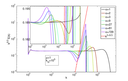
Figure 1: (Color online) Log-log plots of the compensated spectrum $k^{5/3}E(k)$ versus $k$ from a numerical integration of the hyperviscous EDQNM Eq. (4) for different values of $\alpha$; inset: enlarged spectra showing a secondary bottleneck (see text).

Our results apply to compressible flows also. We have studied the simplest instance, that is the unforced hyperviscous 1D Burgers equation (1) . Its solution converges to the entropy solution, i.e., the standard solution with shocks, obtained when ${k_{\scriptscriptstyle\mathrm{G}}}\to\infty$ for any $\alpha\geq 1$ ET04 . Here we are interested in the large-$\alpha$ behavior at fixed ${k_{\scriptscriptstyle\mathrm{G}}}$. We do not have to resort to closure now since we can solve the primitive equation (1) directly by a pseudospectral method. If we choose a single initial condition the resulting spectrum is noisy because, unlike the ordinary Burgers equation, its Galerkin-truncated version and thus also the high-$\alpha$ versions are believed to be chaotic dynamical systems Majda . So we solve (1) with the two-mode random initial condition $v_{0}(x)=\sin x+\sin(2x+\phi)$, where $\phi$ is distributed uniformly in the interval $[-\pi,\,\pi]$. We use $2^{14}$ collocation points and set $\mu=1$, ${k_{\scriptscriptstyle\mathrm{G}}}=342.1$ and $\alpha=1000$.

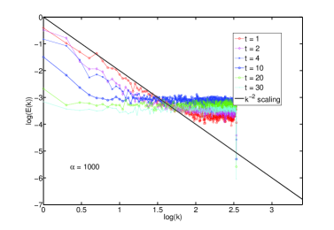
Figure 2: (Color online) Log-log plots of averaged energy spectra (see text) versus wavenumber $k$ for the hyperviscous Burgers equation (1) at various times.

In Fig. 2 we show the Burgers energy spectrum $E(k)=\mid\tilde{v}(k)\mid^{2}$, averaged over 20 realizations of the phase $\phi$ at various times. At the latest output times the spectrum is almost completely flat, i.e., thermalized, with equipartition of the energy between all the Fourier modes. At earlier times $E(k)$ behaves approximately as $k^{-2}$ in an inertial range that corresponds to shocks in physical space; there is a thermalized range at higher wavenumbers up to ${k_{\scriptscriptstyle\mathrm{G}}}$; for $k>{k_{\scriptscriptstyle\mathrm{G}}}$ the spectrum falls very rapidly. No pseudo-dissipation range is observed here between the inertial and thermalized ranges as seen in the 3D NS case (Fig. 1). Perhaps the data are too noisy, but a careful examination of $v(x)$ in physical space indicates that this phenomenon might arise from the compressible nature of the Burgers dynamics: thermalization begins over the whole physical range (as high-frequency noise with wavenumber $\approx{k_{\scriptscriptstyle\mathrm{G}}}$); noise generated close to shocks is absorbed by them and not enough is left to produce any appreciable eddy viscosity that could broaden the shocks.

We now summarize our main findings from the study of hyperviscous hydrodynamical equations with powers $\alpha$ of the Laplacian ranging from unity to very large values.

The simplest results are obtained for very large $\alpha$. The solutions of the 1D Burgers equation or the Navier–Stokes equations in any space dimension $d$ are then very close to the solutions of the corresponding Galerkin-truncated equations, displaying thermalization at wavenumbers below ${k_{\scriptscriptstyle\mathrm{G}}}$. The detailed scenario will of course be affected by the dimension of space. In 3D, with enough resolution, we may be able to observe up to five ranges: an inertial range, a secondary bottleneck, a pseudo-dissipation range, a thermalized range, and a far dissipation range. Because of enstrophy conservation and of the predominance of Fourier-space nonlocal interactions, the 2D case is rather special and deserves a separate study.

The most relevant case is of course that of ordinary dissipation ($\alpha=1$). The energy-spectrum bottleneck generally observed at high Reynolds numbers in 3D incompressible turbulence may be viewed as an incomplete thermalization: as we increase $\alpha$ larger and larger bottlenecks are present, eventually displaying thermalization on their rising side.

We finally deal with the case of moderately large $\alpha$ of the sort used in many simulations hyperviscosity . How safe is this procedure and what kind of artifacts can we expect?

Using large values of $\alpha$ in simulations to “avoid wasting resolution” is hardly advocated by anybody, but we now understand what goes wrong: a huge thermalized bottleneck will develop at high wavenumbers, whose action on smaller wavenumbers is an ordinary $\alpha=1$ dissipation with an eddy viscosity much larger than what would be permissible in a normal $\alpha=1$ simulation.

When $\alpha$ is chosen just a bit larger than unity (e.g. $\alpha=2$ which is standard in oceanography hyperviscosity ) the advantage of widening the inertial range may be offset by artifacts at bottleneck scales; indeed, even an incomplete thermalization will bring the statistical properties of such scales closer to Gaussian, thereby reducing the rather strong intermittency which would otherwise be expected . For similar reasons spurious isotropization can be expected for problems with an anisotropic constraint, such as rapidly rotating or stratified flow or MHD with a strong uniform magnetic field.

We thank J. Bec, R. Benzi, M.E Brachet, W. Bos, J.R. Herring, D. Mitra, K. Khanin, A. Majda, S. Nazarenko, D. Schertzer, E.S. Titi and V. Yakhot for useful discussions. JZZ thanks the CNLS fellows and visitors for many interactions. UF and WP were partially supported by ANR “OTARIE” BLAN07-2_183172. RP and SSR thank DST, JNCASR, and UGC (India) for support and SERC (IISc) for computational resources. UF, RP, and WP are part of the International Collaboration for Turbulence Research (ICTR). SK and JZZ were funded by the Center for Nonlinear Studies LDRD program and the DOE Office of Science Advanced Scientific Computing Research (ASCR) Program in Applied Mathematics Research.

References

- (1) U. Frisch, B. Hasslacher, and Y. Pomeau, Phys. Rev. Lett. 56, 1905 (1986).
- (2) S. Succi, P. Santangelo, and R. Benzi, Phys. Rev. Lett. 60, 2738 (1988).
- (3) C. Cichowlas, P. Bonaïti, F. Debbasch, and M. Brachet, Phys. Rev. Lett. 95, 264502 (2005).
- (4) T. D. Lee, Quart. J. Appl. Math. 10 69 (1952) .
- (5) R. H. Kraichnan, Phys. Fluids 10, 2080 (1967).
- (6) G. Holloway, J. Phys. Oceanogr. 22, 1033 (1992); V. Borue and S.A. Orszag Europhys. Lett. 29, 685 (1995); N.E.L. Haugen and A. Brandenburg, Phys. Rev. E 70, 026405 (2004).
- (7) J.L. Lions, Quelques Méthodes de Résolution des Problèmes aux Limites non Linéaires, Gauthier-Villars (1969).
- (8) R.H. Kraichnan, Phys. Rev. 109, 1407 (1958). While introducing the DIA here, Kraichnan wrote the following about Galerkin truncation: “We may regard this as the introduction of infinite damping (infinite resistance) for the degrees of freedom removed.”
- (9) J. Jiménez, J. Fluid Mech. 279, 169 (1994), notes that “An interesting property of the hyperviscous solutions is the sharpness of their spectral cutoff, which goes from smooth Gaussian …, to a step function in the ultraviscosity limit.”
- (10) J.P. Boyd, J. Sci. Comput. 9, 81 (1994), obtained a truncation result for the linear hyper-diffusion equation.
- (11) S.A. Orszag, Statistical Theory of Turbulence, in Fluid Dynamics, Les Houches 1973, 237, eds. R. Balian and J.L. Peube. Gordon and Breach (1977).
- (12) V. E. Zakharov, V. S. L’vov, and G. Falkovich, Kolmogorov Spectra of Turbulence I, Springer (1992).
- (13) U. Frisch, M. Lesieur, and A. Brissaud, J. Fluid Mech. 65, 145 (1974).
- (14) W. J. T. Bos and J.-P. Bertoglio, Phys. Fluids 18, 071701, 2006.
- (15) J.R. Herring and R.H. Kraichnan, J. Fluid Mech. 91, 581 (1979).
- (16) R. H. Kraichnan, Phys. Fluids 7, 1163 (1964).
- (17) Scheme ETD4RK of C.M. Cox and P.C. Matthews, J. Comput. Phys. 76, 430 (2002).
- (18) M. Lesieur and D. Schertzer, J. de Mécanique. 17, 609 (1978).
- (19) V. L’vov, S. Nazarenko, and O. Rudenko, Phys. Rev. B 76, 024520 (2007).
- (20) S.G. Saddoughi and S.V. Veeravalli, J. Fluid Mech. 268, 333 (1994). As shown by W. Dobler, N.E.L. Haugen, T.A. Yousef and A. Brandenburg, Phys. Rev. E 68, 026304 (2003), the 1D spectrum, generally measured in experiments, may not display a bottleneck even if the 3D spectrum does.
- (21) Z.S. She, G. Doolen, R.H. Kraichnan, and S.A. Orszag, Phys. Rev. Lett. 70, 3251 (1993); Y. Kaneda, T. Ishihara, M. Yokokawa, K. Itakura, and A. Uno, Phys. Fluids, 15, L21 (2003); S. Kurien, M.A. Taylor, and T. Matsumoto, Phys. Rev. E 69, 066313 (2004); J. Schumacher, Europhys. Lett. 80, 54001 (2007); P.D. Mininni, A. Alexakis, and A. Pouquet, Phys. Rev. E 77, 036306 (2008).
- (22) G. Falkovich, Phys. Fluids 6, 1411 (1994); D. Lohse and A. Müller-Groeling, Phys. Rev. Lett. 74, 1747 (1995).
- (23) E. Tadmor, Commun. Math. Sci. 2, pp. 317-324 (2004).
- (24) R. V. Abramov, G. Kovacic, and A. J. Majda, Commun Pure Appl. Math. 56, 1 (2003).