Some exact solutions for the rotational flow
of a generalized second grade fluid between
two circular cylinders

Amir Mahmood${}^{1\,}$, Saifullah¹, Georgiana Bolat²

¹Abdus Salam School of Mathematical Sciences, GC University, Lahore, PAKISTAN
²Technical University of Iasi, R-6600 Iasi, ROMANIA

Abstract

The velocity field and the associated tangential stress corresponding to flow of a generalized second grade fluid between two infinite coaxial circular cylinders, are determined by means of the Laplace and Hankel transforms. At time $t=0$ the fluid is at rest and at $t=0^{+}$ cylinders suddenly begin to rotate about their common axis with a constant angular acceleration. The solutions that have been obtained satisfy the governing differential equations and all imposed initial and boundary conditions. The similar solutions for a second grade fluid and Newtonian fluid are recovered from our general solutions. The influence of the fractional coefficient on the velocity of the fluid is also analyzed by graphical illustrations.

1 Introduction

A large class of real fluids does not exhibit the linear relationship between stress and the rate of strain that is now in great interest of scientists and engineers. Generally, rheological properties of a material are specified by their so called constitutive equations. Among the many constitutive assumptions that have been employed to study non-Newtonian fluid behavior, one class that has gained support from both the experimentalists and the theoreticians is that of Rivlin-Ericksen fluids of second grade. The Cauchy stress tensor T for such fluids is given by [1, 2]

$$\textbf{T}=-p\textbf{I}+\mu\textbf{A}_{1}+\alpha_{1}\textbf{A}_{2}+\alpha_{2}\textbf{A}_{1}^{2}\,,$$ (1)

where $p$ is the pressure, I is the unit tensor, $\mu$ is the dynamic viscosity, $\alpha_{1}$ and $\alpha_{2}$ are the normal stress moduli and $\textbf{A}_{1}$ and $\textbf{A}_{2}$ are the kinematic tensors. In the last years, many authors have made use of rheological equations with fractional derivatives to describe the properties of fluids. The constitutive equations with fractional derivatives have been proved to be a valuable tool to handle viscoelastic properties. In general, these equations are derived from known models by substituting the time ordinary derivatives of stress and strain by derivatives of fractional order.

The constitutive equation of the generalized second grade fluids has the same form as (1), but the kinematic tensor $\textbf{A}_{2}$ is defined by [3-5]

$$\textbf{A}_{2}=D_{t}^{\beta}\textbf{A}_{1}+\textbf{A}_{1}(\mbox{grad}\textbf{v})+(\mbox{grad}\textbf{v})^{T}\textbf{A}_{1}\,,$$ (2)

where v is the velocity field, $\textbf{A}_{1}=\mbox{grad}\textbf{v}+(\mbox{grad}\textbf{v})^{T}$, the superscript $T$ denotes the transpose operator, and $D_{t}^{\beta}$ is the Riemann-Liouville fractional derivative operator defined by [4]

$$D^{\beta}_{t}f(t)=\frac{1}{\Gamma(1-\beta)}\frac{d}{dt}\int_{0}^{t}\frac{f(\tau)}{(t-\tau)^{\beta}}\,d\tau,\,\,\,\,\,\,0<\beta\leq 1\,.$$ (3)

In the above relation $\Gamma(\cdot)$ is the Gamma function. This model reduces to the ordinary second grade fluid when $\beta=1$, because $D^{1}_{t}f=df/dt$.

In this paper, we study the motion of a generalized second grade fluid between two infinite concentric circular cylinders, both cylinders are rotating around their common axis $(r=0)$, with constant angular accelerations. By means of the Laplace and Hankel transforms we obtain the velocity field and the adequate shear stress.

2 Rotational flow between concentric cylinders

Let us consider an incompressible second grade fluid at rest in an annular region between two straight circular cylinders of radii $R_{1}$ and $R_{2}(>R_{1})$. At time $t=0^{+}$, both cylinders suddenly begin to rotate about their common axis with constant angular accelerations. Owing to the shear, the fluid is gradually moved and its velocity in cylindrical coordinated $(r,\theta,z)$ is given by [2,6]

$$\textbf{v}=\textbf{v}(r,t)=\omega(r,t)\textbf{e}_{\theta}\,,$$ (4)

where $\textbf{e}_{\theta}$ is the transverse unit vector. The basic equations corresponding to this motion are [6,7]

$$\tau(r,t)=(\mu+\alpha_{1}D^{\beta}_{t})(\frac{\partial}{\partial r}-\frac{1}{r})\omega(r,t)\,,$$ (5)

$$\frac{\partial\omega(r,t)}{\partial t}=(\nu+\alpha D^{\beta}_{t})\bigg{(}\frac{\partial^{2}}{\partial r^{2}}+\frac{1}{r}\frac{\partial}{\partial r}-\frac{1}{r^{2}}\bigg{)}\omega(r,t),\,\,\,\,\,\,\,\,r\in(R_{1},R_{2}),\,\,\,t>0,$$ (6)

where $\tau(r,t)=S_{r\theta}(r,t)$ is the shear stress which is different of zero, $\nu=\mu/\rho$ is the kinematic viscosity, $\rho$ is the constant density of the fluid and $\alpha=\alpha_{1}/\rho$. The appropriate initial and boundary conditions are

$$\omega(r,0)=0\,,$$ (7)

$$\omega(R_{1},t)=R_{1}\Omega_{1}t,\,\,\,\,\,\,\,\,\,\,\omega(R_{2},t)=R_{2}\Omega_{2}t\,\,\,\,\,\mbox{for}\,\,\,\,t>0\,.$$ (8)

To solve this problem, we shall use as in [7,8] the Laplace and Hankel transforms.

2.1 Calculation of the velocity field

Applying the Laplace transform to Eqs. (6)-(8) and using the Laplace transform formula for sequential fractional derivatives [4], we obtain the following ordinary differential equation

$$(\nu+\alpha q^{\beta})\bigg{[}\frac{\partial^{2}\overline{\omega}(r,q)}{\partial r^{2}}+\frac{1}{r}\frac{\partial\overline{\omega}(r,q)}{\partial r}-\frac{\overline{\omega}(r,q)}{r^{2}}\bigg{]}-q\overline{\omega}(r,q)=0\,,$$ (9)

where the image function $\overline{\omega}(r,q)=\int_{0}^{\infty}\omega(r,t)e^{-qt}dt$  of  $\omega(r,t)$ has to satisfy the conditions

$$\overline{\omega}(R_{1},q)=\frac{R_{1}\Omega_{1}}{q^{2}}\,,\,\,\,\,\,\,\,\,\overline{\omega}(R_{2},q)=\frac{R_{2}\Omega_{2}}{q^{2}}\,,$$ (10)

$q$ being the transform parameter.

We denote by $\overline{\omega}_{{}_{H}}(r_{n},q)=\int_{R_{1}}^{R_{2}}r\overline{\omega}(r,q)B_{1}(rr_{n})dr$, the Hankel transform of the function $\overline{\omega}(r,q)$, where

$$B_{1}(rr_{n})=J_{1}(rr_{n})Y_{1}(R_{2}r_{n})-J_{1}(R_{2}r_{n})Y_{1}(rr_{n}),$$

and $r_{n}$ are the positive roots of the transcendental equation $B_{1}(R_{1}r)=0$ and $J_{1}(\cdot)$ and $Y_{1}(\cdot)$ are Bessel functions of order one of the first and second kind. Applying the Hankel transform to Eq. (9), taking into account the conditions (10) and using the following relations

$$\frac{d}{dr}[B_{1}(rr_{n})]=r_{n}[J_{0}(rr_{n})Y_{1}(R_{2}r_{n})-J_{1}(R_{2}r_{n})Y_{0}(rr_{n})]-\frac{1}{r}B_{1}(rr_{n})$$ (11)

and

$$J_{0}(z)Y_{1}(z)-J_{1}(z)Y_{0}(z)=-\frac{2}{\pi z}\,,$$ (12)

we find that

$$(\nu+\alpha q^{\beta})\bigg{\{}\frac{2[R_{2}\Omega_{2}J_{1}(R_{1}r_{n})-R_{1}\Omega_{1}J_{1}(R_{2}r_{n})]}{\pi q^{2}J_{1}(R_{1}r_{n})}-r_{n}^{2}\overline{\omega}_{{}_{H}}(r_{n},q)\bigg{\}}-q\overline{\omega}_{{}_{H}}(r_{n},q)=0,$$

or equivalently

$$\overline{\omega}_{{}_{H}}(r_{n},q)=\frac{2[R_{2}\Omega_{2}J_{1}(R_{1}r_{n})-R_{1}\Omega_{1}J_{1}(R_{2}r_{n})]}{\pi J_{1}(R_{1}r_{n})}\frac{\nu+\alpha q^{\beta}}{q^{2}[q+\alpha r_{n}^{2}q^{\beta}+\nu r_{n}^{2}]}\,.$$ (13)

Eq. (13) can be written in the following equivalent form

$$\overline{\omega}_{{}_{H}}(r_{n},q)=\overline{\omega}_{{}_{1H}}(r_{n},q)+\overline{\omega}_{{}_{2H}}(r_{n},q)\,,$$ (14)

where

$$\overline{\omega}_{{}_{1H}}(r_{n},q)=\frac{2}{\pi r_{n}^{2}}\frac{R_{2}\Omega_{2}J_{1}(R_{1}r_{n})-R_{1}\Omega_{1}J_{1}(R_{2}r_{n})}{J_{1}(R_{1}r_{n})}\frac{1}{q^{2}}\,,$$ (15)

and

$$\overline{\omega}_{{}_{2H}}(r_{n},q)=-\frac{2}{\pi r_{n}^{2}}\frac{R_{2}\Omega_{2}J_{1}(R_{1}r_{n})-R_{1}\Omega_{1}J_{1}(R_{2}r_{n})}{J_{1}(R_{1}r_{n})}\frac{1}{q[q+\alpha r_{n}^{2}q^{\beta}+\nu r_{n}^{2}]}\,.$$ (16)

The inverse Hankel transforms of the functions $\overline{\omega}_{{}_{1H}}$ and $\overline{\omega}_{{}_{2H}}$ are

$$\overline{\omega}_{{}_{1}}(r,q)=\frac{\Omega_{1}R_{1}^{2}(R_{2}^{2}-r^{2})+\Omega_{2}R_{2}^{2}(r^{2}-R_{1}^{2})}{(R_{2}^{2}-R_{1}^{2})r}\,,$$ (17)

respectively,

$$\overline{\omega}_{{}_{2}}(r,q)=\frac{\pi^{2}}{2}\sum_{n=1}^{\infty}\frac{r_{n}^{2}J_{1}^{2}(R_{1}r_{n})B_{1}(rr_{n})}{J_{1}^{2}(R_{1}r_{n})-J_{1}^{2}(R_{2}r_{n})}\overline{\omega}_{{}_{2H}}(r_{n},q)\,.$$ (18)

Now, we find that the function $\overline{\omega}(r,q)$ has the form

$$\overline{\omega}(r,q)=\frac{\Omega_{1}R_{1}^{2}(R_{2}^{2}-r^{2})+\Omega_{2}R_{2}^{2}(r^{2}-R_{1}^{2})}{(R_{2}^{2}-R_{1}^{2})r}\frac{1}{q^{2}}-$$

$$-\pi\sum_{n=1}^{\infty}\frac{J_{1}(R_{1}r_{n})[R_{2}\Omega_{2}J_{1}(R_{1}r_{n})-R_{1}\Omega_{1}J_{1}(R_{2}r_{n})]B_{1}(rr_{n})}{J_{1}^{2}(R_{1}r_{n})-J_{1}^{2}(R_{2}r_{n})}\frac{1}{q[q+\alpha r_{n}^{2}q^{\beta}+\nu r_{n}^{2}]}\,.$$ (19)

We introduce the notation

$$F(q)=\frac{1}{q[q+\alpha r_{n}^{2}q^{\beta}+\nu r_{n}^{2}]}\,,$$ (20)

and rewrite Eq. (20) in the equivalent form

$$F(q)=\frac{q^{-1-\beta}}{(q^{1-\beta}+\alpha r_{n}^{2})+\nu r_{n}^{2}q^{-\beta}}=\sum_{k=0}^{\infty}(-\nu r_{n}^{2})^{k}\frac{q^{-1-\beta-k\beta}}{(q^{1-\beta}+\alpha r_{n}^{2})^{k+1}}\,.$$ (21)

In order to determine the inverse Laplace transform of the function $\overline{\omega}(r,t)$ we will use the following formulae [9]

$$L^{-1}\bigg{\{}\frac{1}{q^{a}}\bigg{\}}=\frac{t^{a-1}}{\Gamma(a)}\,,\,\,\,\,\,a>0\,,$$

$$L^{-1}\bigg{\{}\frac{q^{b}}{(q^{a}-d)^{c}}\bigg{\}}=G_{a,b,c}(d,t)=\sum_{j=0}^{\infty}\frac{\Gamma(c+j)d^{j}}{\Gamma(c)\Gamma(j+1)}\frac{t^{(c+j)a-b-1}}{\Gamma[(c+j)a-b]}\,,\,\,\,\,Re(ac-b)>0\,.$$

So we find that the velocity field $\omega(r,t)$ has the following form

$$\omega(r,t)=\frac{\Omega_{1}R_{1}^{2}(R_{2}^{2}-r^{2})+\Omega_{2}R_{2}^{2}(r^{2}-R_{1}^{2})}{(R_{2}^{2}-R_{1}^{2})r}t-$$

$$-\pi\sum_{n=1}^{\infty}\frac{J_{1}(R_{1}r_{n})[R_{2}\Omega_{2}J_{1}(R_{1}r_{n})-R_{1}\Omega_{1}J_{1}(R_{2}r_{n})]B_{1}(rr_{n})}{J_{1}^{2}(R_{1}r_{n})-J_{1}^{2}(R_{2}r_{n})}\times$$

$$\times\sum_{k=0}^{\infty}(-\nu r_{n}^{2})^{k}G_{1-\beta,-1-\beta-k\beta,k+1}(-\alpha r_{n}^{2},t)\,,$$ (22)

or, the equivalently

$$\omega(r,t)=\frac{\Omega_{1}R_{1}^{2}(R_{2}^{2}-r^{2})+\Omega_{2}R_{2}^{2}(r^{2}-R_{1}^{2})}{(R_{2}^{2}-R_{1}^{2})r}t-$$

$$-\pi\sum_{n=1}^{\infty}\frac{J_{1}(R_{1}r_{n})[R_{2}\Omega_{2}J_{1}(R_{1}r_{n})-R_{1}\Omega_{1}J_{1}(R_{2}r_{n})]B_{1}(rr_{n})}{J_{1}^{2}(R_{1}r_{n})-J_{1}^{2}(R_{2}r_{n})}\times$$

$$\times\sum_{j,k=0}^{\infty}\frac{(-\nu r_{n}^{2})^{k}(-\alpha r_{n}^{2})^{j}\Gamma(k+j+1)}{\Gamma(k+1)\Gamma(j+1)}\frac{t^{(1-\beta)j+k+1}}{\Gamma[(1-\beta)j+k+2]}\,.$$ (23)

2.2 Calculation of the shear stress

The shear stress $\tau(r,t)$ is obtained from Eqs. (5) and (23) by means of the Laplace transform. From Eq. (5) we find that

$$\overline{\tau}(r,q)=(\mu+\alpha_{1}q^{\beta})(\frac{\partial}{\partial r}-\frac{1}{r})\overline{\omega}(r,q)\,.$$ (24)

Now, applying the Laplace transform to Eq. (23), differentiating the result with respect to $r$ and using Eq. (11), we obtain

$$\overline{\tau}(r,q)=\frac{2R_{1}^{2}R_{2}^{2}(\Omega_{2}-\Omega_{1})}{(R_{2}^{2}-R_{1}^{2})r^{2}}(\mu\frac{1}{q^{2}}+\alpha_{1}\frac{1}{q^{2-\beta}})+\pi\sum_{n=1}^{\infty}\bigg{[}\frac{2}{r}B_{1}(rr_{n})-r_{n}B(rr_{n})\bigg{]}\times$$

$$\times\frac{J_{1}(R_{1}r_{n})[R_{2}\Omega_{2}J_{1}(R_{1}r_{n})-R_{1}\Omega_{1}J_{1}(R_{2}r_{n})]}{J_{1}^{2}(R_{1}r_{n})-J_{1}^{2}(R_{2}r_{n})}\sum_{j,k=0}^{\infty}\frac{(-\nu r_{n}^{2})^{k}(-\alpha r_{n}^{2})^{j}\Gamma(k+j+1)}{\Gamma(k+1)\Gamma(j+1)}\times$$

$$\times\bigg{[}\mu\frac{1}{q^{(1-\beta)j+k+2}}+\alpha_{1}\frac{1}{q^{(1-\beta)j+k+2-\beta}}\bigg{]}\,,$$ (25)

where

$$B(rr_{n})=J_{0}(rr_{n})Y_{1}(R_{2}r_{n})-J_{1}(R_{2}r_{n})Y_{0}(rr_{n})\,.$$

Applying inverse Laplace transform to the image function $\overline{\tau}(r,q)$, we find the shear stress

$$\tau(r,t)=\frac{2R_{1}^{2}R_{2}^{2}(\Omega_{2}-\Omega_{1})}{(R_{2}^{2}-R_{1}^{2})r^{2}}(\mu t+\frac{\alpha_{1}t^{1-\beta}}{\Gamma(2-\beta)})+\pi\sum_{n=1}^{\infty}\bigg{[}\frac{2}{r}B_{1}(rr_{n})-r_{n}B(rr_{n})\bigg{]}\times$$

$$\times\frac{J_{1}(R_{1}r_{n})[R_{2}\Omega_{2}J_{1}(R_{1}r_{n})-R_{1}\Omega_{1}J_{1}(R_{2}r_{n})]}{J_{1}^{2}(R_{1}r_{n})-J_{1}^{2}(R_{2}r_{n})}\sum_{j,k=0}^{\infty}\frac{(-\nu r_{n}^{2})^{k}(-\alpha r_{n}^{2})^{j}\Gamma(k+j+1)}{\Gamma(k+1)\Gamma(j+1)}\times$$

$$\times\bigg{[}\mu\frac{t^{(1-\beta)j+k+1}}{\Gamma[(1-\beta)j+k+2]}+\alpha_{1}\frac{t^{(1-\beta)j+k+1-\beta}}{\Gamma[(1-\beta)j+k+2-\beta]}\bigg{]}\,.$$ (26)

3 Limiting case $(\beta=1)$

Making $\beta=1$ into Eq. (22) we obtain the velocity field

$$\omega(r,t)=\frac{\Omega_{1}R_{1}^{2}(R_{2}^{2}-r^{2})+\Omega_{2}R_{2}^{2}(r^{2}-R_{1}^{2})}{(R_{2}^{2}-R_{1}^{2})r}t-$$

$$-\pi\sum_{n=1}^{\infty}\frac{J_{1}(R_{1}r_{n})[R_{2}\Omega_{2}J_{1}(R_{1}r_{n})-R_{1}\Omega_{1}J_{1}(R_{2}r_{n})]B_{1}(R_{1}r_{n})}{J_{1}^{2}(R_{1}r_{n})-J_{1}^{2}(R_{2}r_{n})}\times$$

$$\times\sum_{k=0}^{\infty}(-\nu r_{n}^{2})^{k}G_{0,-2-k,k+1}(-\alpha r_{n}^{2},t)\,,$$ (27)

corresponding to an ordinary second grade fluid, performing the same motion. Similarly, from (26), we obtain the associated shear stress

$$\tau(r,t)=\frac{2R_{1}^{2}R_{2}^{2}(\Omega_{2}-\Omega_{1})}{(R_{2}^{2}-R_{1}^{2})r^{2}}(\mu t+\alpha_{1})+\pi\sum_{n=1}^{\infty}\bigg{[}\frac{2}{r}B_{1}(rr_{n})-r_{n}B(rr_{n})\bigg{]}\times$$

$$\times\frac{J_{1}(R_{1}r_{n})[R_{2}\Omega_{2}J_{1}(R_{1}r_{n})-R_{1}\Omega_{1}J_{1}(R_{2}r_{n})]}{J_{1}^{2}(R_{1}r_{n})-J_{1}^{2}(R_{2}r_{n})}\sum_{j,k=0}^{\infty}\frac{(-\nu r_{n}^{2})^{k}(-\alpha r_{n}^{2})^{j}\Gamma(k+j+1)}{\Gamma(k+1)\Gamma(j+1)}\times$$

$$\times\bigg{[}\mu\frac{t^{k+1}}{\Gamma(k+2)}+\alpha_{1}\frac{t^{k}}{\Gamma(k+1)}\bigg{]}\,,$$ (28)

The above relations can be simplified if we use the following relations:

$$\sum_{k=0}^{\infty}(-\nu r_{n}^{2})^{k}G_{0,-2-k,k+1}(-\alpha r_{n}^{2},t)=\sum_{k=0}^{\infty}(-\nu r_{n}^{2})^{k}\sum_{j=0}^{\infty}\frac{(-\alpha r_{n}^{2})^{j}\Gamma(k+j+1)}{\Gamma(k+1)\Gamma(j+1)}\frac{t^{k+1}}{\Gamma(k+2)}=$$

$$=\sum_{k=0}^{\infty}\frac{(-\nu r_{n}^{2})^{k}t^{k+1}}{\Gamma(k+2)}\frac{1}{(1+\alpha r_{n}^{2})^{k+1}}=-\frac{1}{\nu r_{n}^{2}}\sum_{k=0}^{\infty}\frac{1}{(k+1)!}\bigg{(}-\frac{\nu r_{n}^{2}t}{1+\alpha r_{n}^{2}}\bigg{)}^{k+1}=$$

$$=\frac{1}{\nu r_{n}^{2}}\bigg{[}1-\exp\bigg{(}-\frac{\nu r_{n}^{2}t}{1+\alpha r_{n}^{2}}\bigg{)}\bigg{]}\,.$$

As a result, we find that, the velocity field has the form

$$\omega(r,t)=\frac{\Omega_{1}R_{1}^{2}(R_{2}^{2}-r^{2})+\Omega_{2}R_{2}^{2}(r^{2}-R_{1}^{2})}{(R_{2}^{2}-R_{1}^{2})r}t-$$

$$-\frac{\pi}{\nu}\sum_{n=1}^{\infty}\frac{J_{1}(R_{1}r_{n})[R_{2}\Omega_{2}J_{1}(R_{1}r_{n})-R_{1}\Omega_{1}J_{1}(R_{2}r_{n})]}{J_{1}^{2}(R_{1}r_{n})-J_{1}^{2}(R_{2}r_{n})}\frac{B_{1}(rr_{n})}{r_{n}^{2}}\bigg{[}1-\exp\bigg{(}-\frac{\nu r_{n}^{2}t}{1+\alpha r_{n}^{2}}\bigg{)}\bigg{]}\,,$$ (29)

and the shear stress has the form

$$\tau(r,t)=\frac{2R_{1}^{2}R_{2}^{2}(\Omega_{2}-\Omega_{1})}{(R_{2}^{2}-R_{1}^{2})r^{2}}(\mu t+\alpha_{1})+\pi\sum_{n=1}^{\infty}\bigg{[}\frac{2}{r}B_{1}(rr_{n})-r_{n}B(rr_{n})\bigg{]}\times$$

$$\times\frac{J_{1}(R_{1}r_{n})[R_{2}\Omega_{2}J_{1}(R_{1}r_{n})-R_{1}\Omega_{1}J_{1}(R_{2}r_{n})]}{J_{1}^{2}(R_{1}r_{n})-J_{1}^{2}(R_{2}r_{n})}\bigg{\{}\frac{\mu}{\nu r_{n}^{2}}\bigg{[}1-\exp\bigg{(}-\frac{\nu r_{n}^{2}t}{1+\alpha r_{n}^{2}}\bigg{)}\bigg{]}+$$

$$+\frac{\alpha_{1}}{1+\alpha r_{n}^{2}}\exp\bigg{(}-\frac{\nu r_{n}^{2}t}{1+\alpha r_{n}^{2}}\bigg{)}\bigg{\}}\,.$$ (30)

Eqs. (29) and (30) are identical with those obtained by Fetecau et al [6 , Eqs. (3.12) and (3.16) for $\lambda\rightarrow 0$]. Making $\alpha\rightarrow 0$ into Eqs. (29) and (30), the similar solutions corresponding to the Newtonian fluid, performing the same motion, are recovered. Making $\Omega_{1}=0$ and $\Omega_{2}=\Omega$ or $\Omega_{1}=\Omega$ and $\Omega_{2}=0$ into Eqs. (23) and (26), we obtain the velocity field and the adequate shear stress corresponding to the flow between two cylinders, one of them being at rest.

4 Conclusion and numerical results

In this paper we establish exact solutions for the velocity field and shear stress corresponding to the flow of a generalized second grade fluid between two concentric circular cylinders. The motion is produced by the two cylinders which at time $t=0^{+}$ begin to rotate around their common axis with angular velocities $\Omega_{1}t$ and $\Omega_{2}t$. The solutions, obtained by means of Laplace and Hankel transforms, are presented under integral and series forms in terms of the generalized $G$-function, and satisfy all imposed initial and boundary conditions. For $\beta=1$ or $\beta=1$ and $\alpha=0$, the similar solutions for the ordinary second grade fluids, respectively, Newtonian fluids are recovered. The velocity field and adequate shear stress corresponding to the flow between two cylinders, one of them being at rest, are obtained as particular cases of our general solutions. Making $\Omega_{1}=0$ and $\Omega_{2}=\Omega$ into Eqs. (23), for instance, we obtain the velocity field

$$\omega(r,t)=\frac{\Omega R_{2}^{2}(r^{2}-R_{1}^{2})}{(R_{2}^{2}-R_{1}^{2})r}t-\pi R_{2}\Omega\sum_{n=1}^{\infty}\frac{J_{1}^{2}(R_{1}r_{n})B_{1}(rr_{n})}{J_{1}^{2}(R_{1}r_{n})-J_{1}^{2}(R_{2}r_{n})}\times$$

$$\times\sum_{j,k=0}^{\infty}\frac{(-\nu r_{n}^{2})^{k}(-\alpha r_{n}^{2})^{j}\Gamma(k+j+1)}{\Gamma(k+1)\Gamma(j+1)}\frac{t^{(1-\beta)j+k+1}}{\Gamma[(1-\beta)j+k+2]}\,,$$ (31)

corresponding to the flow between cylinders, the inner cylinder being at rest.

Finally, the numerical results are given to illustrate the influence of the fractional parameter $\beta$ on the velocity $\omega(r,t)$. In all figures we considered $R_{1}=1$, $R_{2}=4$, $\Omega_{1}=3$, $\Omega_{2}=1.5$, $\rho=1260$, $\alpha_{1}=11.34$ and $\mu=1.48$.

In Figs. 1 the profiles of the velocity $\omega(r,t)$, corresponding to the motion of Newtonian fluid (the curve $\omega\mbox{N}(r)$), second grade fluid (the curve $\omega\mbox{SG}(r)$)) and generalized second grade fluid (the curves $\omega 1(r),\omega 2(r)\,\,\,\mbox{and}\,\,\,\omega 3(r)$), are plotted, for different values of the fractional coefficient $\beta$ and time $t$. It is clearly seen from these figures that velocity increases when the fractional coefficient decreases. Moreover, the influence of $\beta$ is more strong near boundary of the domain and the generalized second grade fluid flows faster than the second grade and Newtonian fluids.

Figs. 2 depict the histories of the velocity field $\omega(r,t)$ at the positions $r=1.3,\,2.5\,\,\,\mbox{and}\,\,\,3.8$, for $t\in[0,10]$ and different values of $\beta$. One can see that the influence of $\beta$ is more strong near boundary of the domain and the velocity increases when $\beta$ decreases. The units of the parameter in Figs. 1-2 are from SI units and the roots $r_{n}$ have been approximated by $n\pi/(R_{2}-R_{1})$ [10].

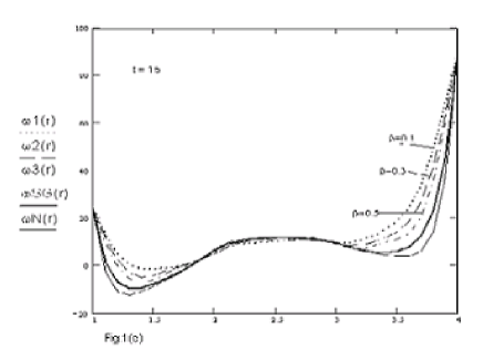
Figure 1: Velocity profile $\omega(r)$ for different values of the fractional coefficient $\beta$

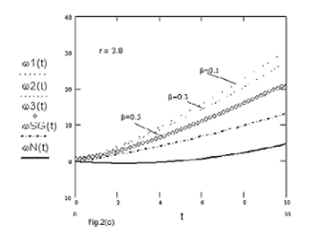
Figure 2: Time variation of the velocity

References

• [1] K. R. Rajagopal, A note on unsteady unidirectional flows of a non-Newtonian fluid, Int. J. Non-Linear Mech. 17 (1982) 369-373.
• [2] C. Fetecau, Corina Fetecau, Starting solutions for the motion of a second grade fluid due to longitudinal and torsional oscillations of a circular cylinder, Int. J. Eng. Sci. 44 (2006) 788-796.
• [3] M. Khan, S. Nadeem, T. Hayat, A. M. Siddiqui, Unsteady motion of a generalized second grade fluid, Math. Comput. Modell. 41 (2005) 629-637.
• [4] R. Hilfer, Applications of Fractional Calculus in Physics, World Scientific Press, Singapore, 2000.
• [5] H. Qi, M. Xu, Stokes’ first problem for a viscoelastic fluid with the generalized Oldroyd-B model, Acta Mech. Sin. (2007), DOI: 10.1007/s10409-007-0093-2.
• [6] C. Fetecau, Corina Fetecau, D. Vieru, On some helical flows of Oldroyd-B fluids, Acta Mech. 189 (2007) 53-63.
• [7] C. Fetecau, A. Mahmood, Corina Fetecau, D. Vieru, Some exact solutions for the helical flow of a generalized Oldroyd-B fluid in a circular cylinder, Sent for publication in Comp. & Appl. Math.
• [8] D. Tong, Y. Liu, Exact solutions for the unsteady rotational flow of non-Newtonian fluid in an annular pipe, Int. J. Eng. Sci. 43 (2005) 281-289.
• [9] C. F. Lorenzo. T. T. Hartley, Generalized Functions for the Fractional Calculus, NASA/TP-1999-209424/Rev1, 1999.
• [10] L. Debnath, D. Bhatta, Integral Transforms and Their Applications (Second Edition), Chapman & Hall/CRC, 2007.