Comparative experimental study of local mixing of active and passive scalars in turbulent thermal convection

Abstract

We investigate experimentally the statistical properties of active and passive scalar fields in turbulent Rayleigh-Bénard convection in water, at $Ra\sim 10^{10}$. Both the local concentration of fluorescence dye and the local temperature are measured near the sidewall of a rectangular cell. It is found that, although they are advected by the same turbulent flow, the two scalars distribute differently. This difference is twofold, i.e. both the quantities themselves and their small-scale increments have different distributions. Our results show that there is a certain buoyant scale based on time domain, i.e. the Bolgiano time scale $t_{B}$, above which buoyancy effects are significant. Above $t_{B}$, temperature is active and is found to be more intermittent than concentration, which is passive. This suggests that the active scalar possesses a higher level of intermittency in turbulent thermal convection. It is further found that the mixing of both scalar fields are isotropic for scales larger than $t_{B}$ even though buoyancy acts on the fluid in the vertical direction. Below $t_{B}$, temperature is passive and is found to be more anisotropic than concentration. But this higher degree of anisotropy is attributed to the higher diffusivity of temperature over that of concentration. From the simultaneous measurements of temperature and concentration, it is shown that two scalars have similar autocorrelation functions and there is a strong and positive correlation between them.

I Introduction

In the studies of hydrodynamic turbulence, scalar field has been one of the main subjects besides the velocity field. This is partly because a scalar field is presumed to be easier to tackle with than a vector field, both experimentally and theoretically. In general, there are two main kinds of scalar fields, classified according to the interaction between the scalar and its carrier flow: One is active scalar which couples dynamically to the velocity field and the other is passive scalar whose feedback to the flow is negligible. Although both are governed by the same advection-diffusion equation, active and passive scalars belong to different realms of mathematics and physics. Due to the dynamical coupling with the advecting velocity field, the problem of active scalars is a nonlinear one. On the other hand, passive scalars obey a linear equation because of the absence of the feedback to the advecting velocity field. This allows a fully theoretical treatment of the problem, which has been carried out recently Shraiman and Siggia (2000); Falkovich et al. (2001). To study the properties of both scalar fields, the turbulent Rayleigh-Bénard convection (RBC), a paradigm for studying buoyancy-driven turbulent flows Castaing et-al. (1989); Sigga (1994); Niemela et-al. (2000); Grossmann and Lohse (2000); Kadanoff (2001), provides an ideal platform. This is because in this system the temperature field itself is already an active scalar, as it drives the turbulent flow via buoyancy, and, if a fluorescent dye solution is injected into the flow, the concentration field of the dye behaves as a passive scalar. The object of the present experimental investigation is to address the following questions: What are the relations, similarities, and differences between the active and passive scalar fields advected by the same turbulent flow?

Passive scalars have been studied extensively for many years, and the results have provided many insights into the turbulence problem Sreenivasan (1991); Shraiman and Siggia (2000); Warhaft (2000); Falkovich et al. (2001). However, there have been a limited number of studies on the relations between the active and passive scalar fields. Celani et al. Celani et-al. (2004) compared the behaviors of active and passive scalars in four different numerical systems Celani et-al. (2002a, b, 2004) by focusing on the issue of universality and scalings and their results provide two possible scenarios: the first is that active and passive fields in the same flow should share the same statistics if the statistical correlations between scalar forcing and carrier flow are sufficiently week; whereas in the second scenario these two fields may behave very differently for systems with strong correlations between the active scalar input and the particle trajectories. These authors thus suggested that a case-by-case study is needed. For thermal convection, Celani et al. Celani et-al. (2002a, 2004) showed that in 2D numerical convective turbulence the two scalar fields have the same even-order anomalous correlations, which are universal with respect to the choice of external sources, and their intermittency in such systems may be traced back to the existence of statistically preserved structures. However, these authors also argued that the equivalence of the statistics of active and passive scalar fields depend crucially on the statistics of the whole velocity field, which may not hold in 3D convective turbulence. Ching et al. Ching et-al. (2003) also offered numerical evidence in the context of simplified shell models for turbulent convection to show that under generic conditions the even-order correlation functions of active scalars can be understood via the emerging theory of statistically preserved structures of the passive scalar counterpart. For magnetohydrodynamics, Celani et al. Celani et-al. (2002b, 2004) showed that a passive scalar displays a direct cascade towards the small scales while the active magnetic potential builds up large-scale structures in an inverse cascade process. Gilbert and Mitra Gilbert and Mitra (2004) further found that active and passive fields have different scaling properties in the framework of a shell model. Ching et al. Ching et-al. (2003) argued that such different scaling behaviors are due to the fact that the active equations possess additional conservation laws and the zero modes of the passive problem is not the leading factor that dominates the structure functions of the active field. However, some of the above fundamental relations between active and passive scalar fields have not been investigated experimentally.

In an earlier study, Zhou and Xia Zhou and Xia (2002) investigated experimentally the mixing of an active scalar, i.e. the temperature field, in thermal turbulence. Their results show that the active scalar field has sharp fronts or gradients with similar statistical properties as those found in passive scalars, such as the saturation of structure function exponent and log-normal distribution of the width of fronts. However, to the best of our knowledge, there have been no experimental investigation to directly compare the fundamental properties of active and passive scalars that are driven by the same turbulent velocity field. In this paper, we undertake such studies in a turbulent RBC system and our results suggest that the active scalar possesses a higher level of intermittency.

The remainder of this paper is organized as follows. In Sec. II, we describe the convection cell used in the experiments, details of the temperature measurement and the technique of laser-induced fluorescence (LIF), and experimental conditions and parameters. The experimental results are presented and analyzed in Sec. III, which is divided into five parts. Sec. III.1 and III.2 discuss the statistical properties of local concentration and temperature fluctuations, respectively. In Sec. III.3 we show that there is a certain buoyant scale in turbulent thermal convection, above which buoyancy effects are important and temperature is active. Sec. III.4 compares the levels of intermittency and isotropy of the two scalars, both above and below the buoyant scale. Sec. III.5 studies the cross-correlation between the two scalars. We summary our findings and conclude in Sec. IV.

II Experimental setup and procedures

II.1 Convection cell

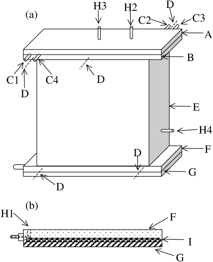
Figure 1: Schematic diagram of the rectangular cell. (a) Front view of the rectangular cell and (b) cross-section view of the bottom plate. A: the chamber cover, B: the top plate, C1, C2, C3, C4: nozzles, D: thermistors, E: the Plexiglas sidewall, F: the bottom plate, G: the cover for the bottom plate, H1: slit for dye injection, H2: nozzle for dilution water injection, H3: nozzle for inserting the small thermistor, H4: nozzle for fluid out-flowing, I: heater.

The scalar measurements were conducted in a rectangular turbulent RBC cell, whose schematic drawing is shown in Fig. 1. The length, width and height of the cell are $25.4\times 7.5\times 25.4$ cm³, respectively, and thus the large-scale circulation (LSC) is confined in the plane with the aspect ratio unity Xia et-al. (2003); Zhou et-al. (2007); Sun et-al. (2008). The sidewall of the cell, indicated as E in the figure, is composed by four transparent Plexiglas plates of thickness $7$ mm. The top (B) and bottom (F) plates, whose surfaces are electroplated with Nickel to prevent the oxidation by water, are made of copper with a thickness of $1.5$ cm for its good thermal conductivity ($400$ W/mK). Rubber O-rings are placed between the copper plates and the sidewall plates to avoid fluid leakage. A water chamber is constructed with the upper surface of the top plate and an attached stainless cover (A). There are four nozzles (C1, C2, C3 and C4), located at the end of the long edges, through which a refrigerated circulator is connected to the chamber. To keep the temperature of the upper plate uniform, water is pumped into the chamber through two nozzles C1 and C3, circulates within the chamber, and then goes out from the other two nozzles C2 and C4, respectively. A rectangular film heater (I) is sandwiched between the lower copper plate (F) and a stainless steel plate (G). There is a slit (H1), through which the fluorescence dye solution is injected into the cell, parallel to the short edge and $1$ cm from the sidewall on the lower copper plate. To minimize the perturbation of the bottom plate and the lower boundary layer, the area of the slit for injection $S_{slit}$ is very small, which is $1$ mm in width and 2 cm in length, so the slit takes up only $0.1\%$ of the bottom plate’s total area. Diluted water is injected from the nozzle H2 to keep the background concentration of the cell unchanged and the nozzle H4 is used for water out-flowing.

II.2 Temperature measurements

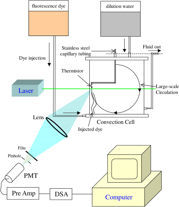
Figure 2: (Color online). Schematic diagram of the experimental setup for simultaneous measurements of temperature and concentration.

There are two different types of thermistors used in our experiments for the temperature measurements. Five thermistors of the first type (Model 44031, Omega Engineering Inc.), indicated as D in Fig. 1, are imbedded inside the two plates to monitor their respective temperatures. Three thermistors are in the top plate and the other two are in the bottom one. A $6.5$-digit multimeter (Model 2000, Keithley Instruments Inc.) is used to record the resistance of the thermistors with a sampling frequency of $\sim 1$ Hz. The measured relative temperature difference between two thermistors in the same plate is found to be less than $2\%$ of that across the convection cell for both plates in our experimental conditions, indicating that the temperature is uniform across the two horizontal plates. The second type of thermistors (AB6E3-B10KA103J, Thermometrics) are used in the local temperature measurement inside the convecting fluid. They have a sensing head of $250$ $\mu m$ in diameter and a thermal time constant of $10$ ms in water, which is fast enough to detect the temperature fluctuations in thermal turbulence. As shown in Fig. 2, the thermistor is threaded through a stainless steel capillary tubing (U143, Fisher Scientific) with outer diameter of $1.5$ mm and inner diameter of $1$ mm and then attached to a translational stage with an accuracy to $0.001$ mm. This arrangement allows the precise adjustment of the separation between the temperature probe and the laser beam, which is used for the local concentration measurement and will be introduced in Sec. II.3.1. A Wheatstone bridge with AC source and a lock-in amplifier (Model SR830 DSP, Stanford Research Systems) are used to measure the temperature fluctuations. A Dynamic Signal Analyzer (DSA, HP 35670A) with a 24-bit dynamic range and four input channels is used to digitize and record the signals and then transmit them to computer.

II.3 LIF technique

There are many experimental techniques for measuring a passive scalar field in turbulent flows, among which the LIF (laser-induced fluorescence) technique seems to provide the best non-intrusive method for the high-spatial-resolution measurement of concentration. The use of this technique in fluid mechanics have been well documented Koochesfahani and Dimotakis (1985); Walker (1987); Prasad and Sreenivasan (1990); Saylor (1995); Catrakis and Dimotakis (1996); Crimaldi (1997); Wang and Fiedler (2000). In almost of all these studies were carried out in open systems, such as turbulent flows in a pipe or in a channel. Whereas, LIF experiments involving longtime measurements in closed systems, such as the turbulent RBC, have not been reported. Longtime measurements in a close system will result in an increase of mean concentration of the system and hence leads reductions in the dynamical range of the fluorescence signal and also in the signal-to-noise ratio. In this section we present the details of the apparatus for our LIF measurements and how we overcome such difficulties, and show the validation of this technique in our case.

II.3.1 Local concentration measurement

Figure 2 shows the schematic diagram of the experimental setup for local concentration measurement. The solution of the fluorescence dye of Rhodamine 6G is injected from the bottom plate of the convection cell, and then a laser light source is used to illuminate the flow. From the absorption spectrum of dye solution with concentration of $1.33\times 10^{-7}$ M measured by a monochromator (Model 300i, Acton Research Corporation) and an ICCD (Model TE/CCD-1024-E/1, Princeton Instruments Inc.), one sees that there is an absorbtion peak of fluorescence dye around the wavelength of $520$ nm. Thus the green light with the wavelength of $514.5$ nm from an argon ion laser (Coherent Innova 70) is chosen as the exciting light. For low concentration, the resulting fluorescence intensity at one point is proportional to the local concentration. We use a photomultiplier tube (PMT, R2368, Hamamatsu) to quantify the intensity of the fluorescence. From the fluorescence spectrum of dye solution measured by the same equipments as for the absorbtion spectrum, there is an emission peak around the wavelength of 560 nm, so a filter with a passband from 550 nm to 570 nm is chosen and is placed in front of the PMT to block out the incident green light. To improve the signal-to-noise ratio, the experiments were conducted in a dark environment to minimize noise due to ambient light and a low-noise preamplifier (Model SR560, Stanford Research Systems) is used to filter out high frequency noise and amplify the signal obtained from PMT. The four-channel DSA, which is also used for recording the temperature fluctuations, digitizes and records the fluorescence signals and then transmits them to computer.

Since the turbulent RBC is a closed system, a continuous injection of dye will increase the background concentration level in the convection cell and thus reduce the dynamical range of the fluorescence signal. To solve this problem, we injected dilution water into the cell to keep the background concentration constant. As shown in Fig. 2, both the dye solution and dilution water are supplied to the cell from the raised tanks and by the pressure difference between the tanks and the cell and hence the flow rate of injected fluids can be varied by changing the height of the tanks. The out-flowing fluid is captured in a third tank (not shown in the figure) from the nozzle H4 in Fig. 1. To minimize the perturbation of the flow field in the convection cell, the speed of injected fluids is approximately the same as that of the large-scale circulation (LSC) of the convective flow, which is about 1 cm/s in our case. In the present case, the volume of injected fluids per unit time is very small (about $0.2$ mL/s for the dye solution and about $0.4$ mL/s for the dilution water, in contrast to the convecting fluid volume of $4.84$ L).

II.3.2 Calibration for LIF

Previous works have pointed out that there are some effects which can influence LIF measurement and hence change the measured magnitude of the dye concentration Koochesfahani and Dimotakis (1985); Walker (1987); Saylor (1995); Crimaldi (1997); Wang and Fiedler (2000). The effects which we must consider in our experiments are as follows:

PH and temperature effects: The measured fluorescence intensity $I_{f}$ may vary with PH and temperature Walker (1987). However, in our experiment, the PH of the fluid in the convection cell is almost constant ($\sim 5.5$) and the temperature fluctuations at the measuring position is about $2^{\circ}C$. In this range, PH and temperature effects can be neglected.

Absorption along the illumination path: For our optical configuration, the incident laser must pass through the background fluid which itself contains dye in it before illuminating the measuring position. This causes the attenuation of the illumination source along its path due to absorption and then a non-linear relationship between fluorescence intensity and dye concentration Walker (1987); Crimaldi (1997). However for sufficiently low concentration, absorption effects along the incident laser beam path can be neglected and the fluorescence intensity at the measuring position can be expressed linearly as

$$I_{f}=\beta I_{e}C,$$ (1)

where $\beta$ is a proportionality constant, $I_{e}$ is the intensity of the induced laser and $C$ is the dye concentration.

Photobleaching: If the exciting laser intensity is high enough or the velocity $v$ of the fluid is zero or too small for the LIF measurement, some dye molecules, after excited, don’t absorb or re-emit light and the fluorescence intensity decays with time, due to photodecomposition or collision quenching, etc. This phenomenon is called photobleaching and have been well studied in many experiments Koochesfahani and Dimotakis (1985); Saylor (1995); Crimaldi (1997); Wang and Fiedler (2000).

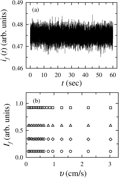
Figure 3: (a) A sample time series of $i_{f}(t)$ measured at the flow cell center. Data taken at $C=2.0\times 10^{-7}$ M, $I_{e}=200$ mW and $\upsilon=0.14$ cm/s. (b) $I_{f}$ ($=\langle i_{f}(t)\rangle$) vs $\upsilon$ at $I_{e}=200$ mW for, from bottom to top, $C=0.5\times 10^{-7}$ M, $1.5\times 10^{-7}$ M, $2.5\times 10^{-7}$ M, and $4.0\times 10^{-7}$ M.

To determine the proper ranges in which our experiments can be carried out properly, we calibrated the fluorescence intensity $I_{f}$ under controlled conditions (e.g. $C$, $I_{e}$ and $v$). The convection cell in Fig. 2 was replaced by a flow cell and a rectangular water tank, which contains dye solution with known concentration, is used as a reservoir. Water was pumped from the tank to the flow cell and then returning back to the tank by a gear pump. The fluorescence intensity was measured at the center point of the flow cell. Assuming a laminar velocity profile, we can obtain the mean velocity at the measuring position from the flow rate of the pump and the cross section area of the flow cell.

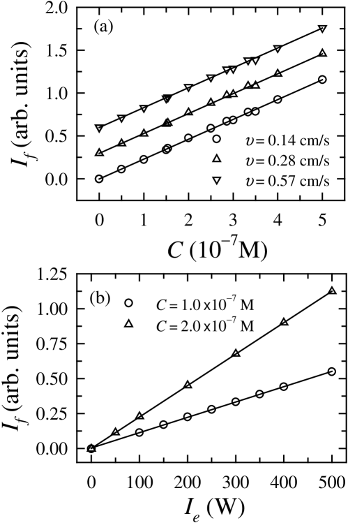
Figure 4: (a) $I_{f}$ vs $C$ at $I_{e}=200$ mW for three different velocities. For clarity, the $\upsilon=0.28$ cm/s and $0.57$ cm/s data have been shifted up by $0.3$ and $0.6$, respectively. (b) $I_{f}$ vs $I_{e}$ at $\upsilon=0.28$ cm/s for two different concentrations. The solid lines show the linear fits to the corresponding data.

A sample time-series of the measured instantaneous fluorescence intensity $i_{f}(t)$ is shown in Fig. 3(a). One sees no attenuation of $i_{f}(t)$ in this 60-second segment. In Fig. 3(b), we show $I_{f}$ ($=\langle i_{f}(t)\rangle$, where $\langle\cdots\rangle$ denotes a time average) measured at different dye concentrations as functions of the flow velocity. We see no appreciable dependence of $I_{f}$ on the fluid velocity $v$. In our scalar experiment, the mean velocity at the measuring position is about 1.8 cm/s at $Ra=1.2\times 10^{10}$ (see Sec. III.5). So in this range of fluid velocity photobleaching effects can be neglected. In Fig. 4(a) we show measured fluorescence intensity, at several flow velocities, vs the concentration $C$. It is seen that, over the range measured ($<5.0\times 10^{-7}$ M), $I_{f}$ is linear with $C$. In Fig. 4(b) $I_{f}$ was measured with increasing incident laser intensity $I_{e}$, which was measured by a power meter (model 1825-C, Newport). For $I_{e}<500$ mW, $I_{f}$ is found to be proportional to $I_{e}$. Based on the above measurements, we chose the concentration of the injected dye solution $C_{0}$ to be 4.0$\times 10^{-7}$ M, the background concentration $C_{back}=1.33\times 10^{-7}$ M and the incident laser intensity $I_{e}=200$ mW in our scalar experiment. In these parameter ranges Eq. (1) is valid and the fluorescence intensity $I_{f}$ is proportional to the local concentration $C$. Thus the local concentration can be obtained directly from the measured fluorescence intensity.

II.4 Experimental conditions and parameters

Table 1: Typical experimental parameters. $\bar{u}$ is determined from the cross-correlation between temperature and concentration fluctuations in Sec. III.5. $t_{B}$ and $t_{0}$ ($\simeq 4H/\bar{u}$) are the Bolgiano time scale and the turnover time of LSC, respectively.

$\Delta T$	$H$	Ra	Pr	Sc	$Pe_{T}$	$Pe_{C}$	Nu
(∘C)	(cm)
27.85	25.4	$1.2\times 10^{10}$	5.3	2100	$3.16\times 10^{4}$	$1.25\times 10^{7}$	140
$T_{bulk}$	$\nu$	$\kappa_{T}$	$\kappa_{C}$	$\bar{u}$	$t_{B}$	$t_{0}$
(∘C)	$(m^{2}/s)$	$(m^{2}/s)$	$(m^{2}/s)$	(cm/s)	(sec)	(sec)
30.97	$7.85\times 10^{-7}$	$1.48\times 10^{-7}$	$3.73\times 10^{-10}$	1.84	1.3	55.2

In our experiments, water is used as the convecting fluid and Rhodamine 6G as the fluorescence dye. During the experiments, the constant power is supplied to the bottom plate of the convection cell, so that it is under a constant-flux boundary condition, but at steady state its temperature remains effectively constant; the top plate’s temperature is regulated so that it is under constant-temperature boundary condition. The control parameters are the Rayleigh number Ra, the Prandtl number Pr and the Schmidt number Sc, which are defined as,

$$Ra=\frac{\alpha g\Delta TH^{3}}{\nu\kappa}\ ,\mbox{\ }Pr=\frac{\nu}{\kappa_{T}}\ ,\mbox{\ and\ }Sc=\frac{\nu}{\kappa_{C}}\ ,$$ (2)

respectively. Here $\alpha$, $\nu$, $\kappa_{C}$, and $\kappa_{T}$ are the coefficients of thermal expansion, kinematic viscosity, molecular diffusivity of the fluorescence dye and thermal diffusivity of the working fluid, respectively, $g$ is the acceleration due to gravity, $\Delta T$ is the temperature difference between the bottom and the top plates of the convection cell, and $H$ is the height of the cell. Another parameter used to characterize the rate of advection of the scalar by a flow to its rate of diffusion is Péclet number, which is defined as,

$$Pe_{T}=\frac{\bar{u}H}{\kappa_{T}}\mbox{\ \ and\ \ }Pe_{C}=\frac{\bar{u}H}{\kappa_{C}}$$ (3)

for temperature and concentration, respectively. Here $\bar{u}$ is the mean velocity at the measuring position. Table I summarizes the typical experimental parameters of the present investigation. From the table, one sees that, although $Pe_{C}$ is two orders larger than $Pe_{T}$, both $Pe_{C}$ and $Pe_{T}$ are much larger than 1, suggesting that the mixing of the temperature and concentration fields are both dominated by the turbulent velocity field, rather than their diffusion rates. Table I also shows that the temperature difference across the cell $\Delta T$ is 27.85^∘C. Previous studies Funfschilling et-al. (2005); Sun et-al. (2005a) have pointed out that to strictly conform to the Boussinesq condition (in water) $\Delta T$ should be limited to $\lesssim$ 15 ^∘C. Thus, there may exist some Non-Boussinesq effect in our current system. Non-Boussinesq effect in water manifests as an increase in the mean bulk temperature as compared to the average of the top and bottom temperatures, and it also slightly reduces the heat flux, i.e. Nusselt number Ahlers et-al. (2006). However, its effect on the temperature and concentration fluctuations are unknown.

In addition to the injection from the bottom plate, the dye solution was also injected into the central region of the convection cell. Due to the absence of the mean flow in the cell center, however, the dye packets meander around after injection and we could not acquire sufficient amount of mixing data (signals) for statical analysis. The measurements were also carried out near the sidewall of a cylindrical cell. Comparable features and behaviors of the passive scalar and of its relations with the active scalar were obtained. However, due to azimuthal meandering of the LSC in the cylindrical cell Sun et-al. (2005b); Brown et-al. (2005); Xi et-al. (2006), the injected dye solution wobbles with the LSC and cannot always pass through the laser beam, resulting in a poor signal-to-noise ratio. The statistics are thus worse for the cylindrical cell. Therefore, all results presented and discussed in this paper are from measurements made near the sidewall of the rectangular cell with dye injected from the bottom plate.

For the present Ra and Pr, the viscous boundary layer thickness near the sidewall is about 2 mm Qiu and Xia (1998). Thus the measuring position is chosen at $1$ cm from the sidewall and at the mid-height of the convection cell, which is outside of the sidewall viscous boundary layer and inside the LSC. The cell is tilted with a small angle of about $1^{\circ}$ near the side of the dye injection slit to lock the LSC and to make the dye solution move upwards with the LSC after it is injected into the cell.

To reveal the statistical properties of passive and active scalars, longtime measurements of the local concentration and temperature fluctuations were carried out independently. The measurement of concentration lasted 27 hours with a sampling frequency of 64 Hz. While the time series of temperature fluctuations, which was obtained at the same measuring position and under the same conditions as concentration, consists of three parts, each of which lasted 20 hours and all were acquired at a sampling rate of 64 Hz. To study the relations between these two scalars, a simultaneous measurement of the local concentration and temperature fluctuations was also made. In this case, the temperature probe (thermistor) was placed above the concentration probe (laser beam). The separation $\ell$ between two probes can be adjusted by a translational stage. For each separation, we recorded two hours of data, except the measurement for $\ell=0.375$ mm which lasted 6 hours, with the sampling frequency of 128 Hz for both concentration and temperature.

III Results and discussion

III.1 The passive scalar measurement

Figure 5: (Color online). (a) A 60-second time series of concentration fluctuations. (b) PDF of concentration fluctuations $P(C)$. The dashed curve represents a Gaussian-function fitting to the background signal and the solid line is for reference.

Figure 5(a) shows a typical time series of the measured concentration fluctuations. When the injected dye packets passing through the concentration probe, a signal with a pulse-like shape would be detected. From the figure, one sees that our measured $C(t)$ consists of many such pulse-like signals of variable heights, corresponding to dye packets with different concentration levels.

In homogeneous turbulent flows, probability density function (PDF) of the velocity fluctuations is Gaussian Jayesh and Warhaft (1991) (It was also showed that the velocity fluctuations in turbulent RB system is Gaussian distributed Qiu et-al. (2004); Sun and Xia (2005)). It is generally assumed that the PDF of a passive scalar is also Gaussian, since it is advected by the Gaussian-distributed turbulent velocity field. Earlier measurements about the scalar PDF in homogeneous turbulence Tavoularis and Corrsin (1981) showed that a Gaussian distribution was a satisfactory model for the scalar signal itself except that the tails of the PDF have not been examined. However, Jayesh $\&$ Warhaft Jayesh and Warhaft (1991) found that for a mean temperature gradient in grid turbulence the tails of the temperature PDF have an exponential shape (in their system temperature is passive). Our measured PDF $P(C)$ is shown in Fig. 5(b). One sees that the PDF consists of two parts. The left part, which has a abscissa value below $-0.25$, is the distribution for the background signals. The distribution of this part is approximately Gaussian, and one can use a Gaussian function to fit the data of this part (the dashed curve in the figure). The right part is the distribution of the mixed fluorescence dye. It can be seen that this part exhibits an exponential decay, which was also observed for passive scalars in other types of turbulent flows, e.g. in a turbulent jet Villermaux et-al. (1998).

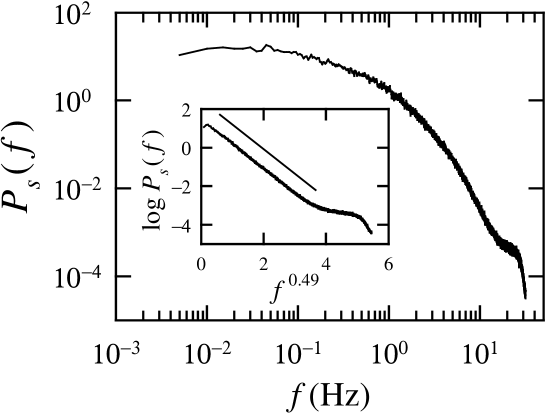
Figure 6: Power spectra $P_{s}(f)$ of the fluctuating concentration $C(t)$. Inset is the plot of $\log[P_{s}(f)]$ as a function of $f^{0.49}$ for the same data. The solid line is for reference.

Figure 6 shows the power spectra $P_{s}(f)$ of the measured dye concentration $C$. The figure shows that the magnitude of $P_{s}(f)$ spans about five decades from the large scale to the noise level. And we see no obvious scaling in the low-frequency range, which may be due to a low Reynolds number (about 5700 in our scalar experiments). At higher frequencies, the measured $P_{s}(f)$ drops sharply and can be fitted by a stretched exponential function

$$P_{s}(f)\sim e^{\displaystyle{[-(f/f_{c})^{b}}]},\mbox{\ \ }b=0.49\pm 0.05$$ (4)

where $f_{c}$ is a cutoff frequency. The inset of Fig. 6 shows a semi-logarithmic plot of the measured $P_{s}(f)$ as a function of $f^{0.49}$. In this plot, the stretched exponential function appears as a straight line. The cut-off frequency of the concentration is around $10\sim 20Hz$, which approximately equals to that of the temperature (see Sec. III.2).

III.2 The active scalar measurement

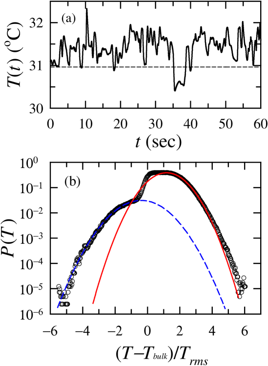
Figure 7: (Color online). (a) A 60-second time series of temperature fluctuations. The dashed line indicates the mean bulk temperature $T_{bulk}$. (b) Corresponding PDF of normalized temperature fluctuations $P(T)$. The dashed curve and the solid curve are two Gaussian-function fittings to the left and right tails, respectively.

Figure 7(a) shows how the temperature fluctuations change with time. The measured $T(t)$ shows many intermittent upward sharp spikes of variable heights, which may be attributed to the upward-moving hot plumes. The corresponding PDF of the normalized temperature fluctuations is shown in Fig. 7(b). Unlike the exponential distributions observed in the center and near the sidewall of a cylindrical cell, the measured PDF near the sidewall in the rectangular cell shows a flat central region and two Gaussian-like tails, which are fitted by separate Gaussian functions (the solid and dashed curves). The Gaussian-like distribution of temperature fluctuations means that the temperature probe felt a lot of thermal coherent structures, i.e. thermal plumes, passing through it Solomon and Gollub (1991). The ratio of the long side to the short side of our rectangular convection cell is about $3.3$, so that the LSC is largely locked in the vertical plane parallel to the long side. Hence most of thermal plumes would group together, move upwards with the LSC and pass through the measuring position due to the confinement in the other direction. Thus, although our experiments with $Ra=1.2\times 10^{10}$ were carried out in the so-call “hard turbulence” regime Castaing et-al. (1989), the measured temperature fluctuations near the sidewall have two Gaussian-like tails rather than exponential ones. It is also not surprising that the right peak is more than ten times higher than the left one, since the LSC has been locked and at the measuring position there are more hot plumes moving upwards than cold one moving downwards. Note also that there is only one group of cold plumes in the 60-second time series shown in Fig. 7(a), as compared to the large number of hot plumes in the same plot.

Figure 8: Power spectra $P_{s}(f)$ of the fluctuating temperature $T(t)$. Inset is the plot of $\log[P_{s}(f)]$ as a function of $f^{0.70}$ for the same data. The solid line is for reference.

We now turn to the power spectra of temperature fluctuations. Based on dimensional arguments, it is traditionally thought that there is simple scaling relation between $P_{s}(k)$ and $k$ in the low-frequency region, i.e.,

$$P_{s}(k)\sim k^{-a},$$ (5)

where $k$ is the wavenumber. Here, $a$ would be $5/3$ according to Kolmogorov’s arguments (K41)Kolmogorov (1941a, b); Obukhov (1949); Corrsin (1951), and it would be $7/5$ if the arguments of Bolgiano R. Bolgiano (1959) and Obukhov A.M. Obukhov (1959) (BO59) are correct. However, from a direct multipoint measurement of the temperatrue field, Sun et al. Sun et-al. (2006) showed that $a=8/5$ near the sidewall of a cylindrical cell, which could be explained by a simple scaling analysis based on the coaction of buoyancy and inertial forces.

Figure 8 shows the measured temperature power spectra $P_{s}(f)$ as a function of $f$. From the figure, one sees that the magnitude of $P_{s}(f)$ spans more than nine decades from the large scale to the noise level. However, the scaling range in the low-frequency region is so limited that one cannot tell the accurate value of $a$. This may be due to the asymmetry of the rectangular cell and the sidewall effect. Another possible reason for this limited scaling range is that the measured $P_{s}(f)$ here is based on time or frequency domain. By using the Taylor frozen-turbulence hypothesis with the condition that the turbulent velocity fluctuations is much smaller than the mean flow velocity, one can relate the time domain results to those of the space domain. However, it is known that the mean flow velocity is comparable to the rms velocity near the sidewall in turbulent RBC convection cell Shang and Xia (2001). This would flatten the measured $P_{s}(f)$ in the low-frequency region. At higher frequencies, the measured $P_{s}(f)$ drops sharply and can be fitted by a stretched exponential function

$$P_{s}(f)\sim e^{\displaystyle{[-(f/f_{c})^{b}}]},\mbox{\ \ }b=0.70\pm 0.05$$ (6)

where $f_{c}$ is a cutoff frequency. (We also used the data measured in a $81\times 20\times 81$-cm³ rectangular cell from Ref. Zhou et-al. (2007) to study the temperature power spectra near the sidewall and $b=0.73\pm 0.05$ was obtained.) Previous measurements of temperature in smooth Wu et-al. (1990) and rough Du and Tong (2001) cylindrical cells also showed a stretched exponential decay at higher frequencies. However, the values of $b$ in those studies are both $0.55\pm 0.05$, which are smaller than our results. Power spectrum of the temperature fluctuations describe the cascade of entropy of the system and hence a larger value of $b$ here means a more rapid cascade of the system’s entropy compared with the cylindrical convection cell. This may be due to the asymmetry of the rectangular cell and the sidewall effect. The inset of Fig. 8 shows a semi-logarithmic plot of the measured $P_{s}(f)$ as a function of $f^{0.70}$. In this plot, the stretched exponential function appears as a straight line. From Fig. 8, one sees that the cut-off frequency of the temperature is around $10\sim 15Hz$, which is about the same as that of concentration as discussed in Sec. III.1.

III.3 The buoyant scale of convective turbulence

In 1959, Bolgiano R. Bolgiano (1959) and Obukhov A.M. Obukhov (1959) proposed that there is a characteristic length scale in buoyancy-driven turbulence, now commonly referred to as the Bolgiano scale $\ell_{B}$, above which buoyancy effects are important. It has been shown Monin and Yaglom (1975) that the Bolgiano scale can be estimated as

$$\ell_{B}=\frac{\epsilon_{v}^{5/4}}{\epsilon_{T}^{3/4}(g\alpha)^{3/2}},$$ (7)

where $\epsilon_{v}$ and $\epsilon_{T}$ are the kinematic and thermal dissipation rates. Note that if the local dissipation rates $\epsilon_{v}(\vec{r})$ and $\epsilon_{T}(\vec{r})$ are used in the above equation, then it gives a local Bolgiano scale. The global Bolgiano scale may be obtained by using the expressions of the globally averaged dissipation rates $\epsilon_{v}$ and $\epsilon_{T}$ in terms of Ra, Pr, and Nu Sigga (1994), which gives:

$$\ell_{B}=\frac{Nu^{1/2}H}{(RaPr)^{1/4}},$$ (8)

As all our measurements are made in the time domain, we use $t_{B}$, which is the counterpart of $\ell_{B}$ in the time domain, as a characteristic time scale in our system, i.e.

$$t_{B}=\frac{Nu^{1/2}t_{0}}{(RaPr)^{1/4}},$$ (9)

which can be easily evaluated from the measured values of Ra, Pr, Nu and the large-scale flow turnover time $t_{0}$.

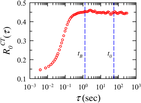
Figure 9: (Color online). Cross-correlation coefficient $R_{0}^{CT}(\tau)$ of the concentration and temperature increments. The two dashed lines show $t_{B}$ and $t_{0}$. The separation $\ell$ between the temperature probe and the laser beam is $0.375$ mm.

To check whether this buoyant scale exists in turbulent RBC, we compute the cross-correlation coefficient $R_{0}^{CT}(\tau)$ between the increments of concentration and temperature, i.e.,

$$R_{0}^{CT}(\tau)=\frac{\langle\delta_{\tau}C(t)\delta_{\tau}T(t+\ell/\bar{u})\rangle}{\delta_{\tau}C(t)_{rms}\delta_{\tau}T(t)_{rms}}$$ (10)

where $\delta_{\tau}C(t)=C(t+\tau)-C(t)$, $\delta_{\tau}T(t)=T(t+\tau)-T(t)$, and $\ell/\bar{u}$ describes the time delay between the concentration and temperature signals due to the separation of the two probes. When the concentration and temperature increments are uncorrelated, we have $R_{0}^{CT}(\tau)=0$, while $R_{0}^{CT}(\tau)=1$ is obtained for a linear relation between the two increments.

Figure 9 shows the measured $R_{0}^{CT}(\tau)$ as a function of $\tau$ for $\ell=0.375$ mm, which is the measured separation between the laser beam and the thermistor tip. Two dashed lines in the figure show $t_{B}$ and $t_{0}$, which were determined from the measured Ra, Pr, and Nu (see Table I) using Eq. (9) and from $4H/\bar{u}$ respectively. One sees that $R_{0}^{CT}(\tau)$ increases with increasing $\tau$ when $\tau$ is small and saturates at a value of $\sim 0.45$ when $\tau\gtrsim t_{B}$. It has been shown previously Ching et-al. (2004) that the vertical velocity increments correlate strongly with the temperature increments above the Bolgiano time scale $t_{B}$, reflecting strong effects of buoyancy. Since the concentration fluctuations are dominated by the vertical velocity field near the sidewall, a large positive correlation between the concentration and temperature increments is expected and indeed observed here. This supports the idea that, above the Bolgiano time scale, buoyancy effects are significant and temperature can be regarded as an active scalar. In contrast, for time scales below $t_{B}$, buoyancy is not important and the temperature field behaves as a passive scalar. Thus, the concentration and temperature fluctuations are two separate stochastic fields at scales below $t_{B}$. In this case, the correlation between them should be very weak (as shown in Fig. 9, $R_{0}^{CT}(\tau)$ decreases sharply when $\tau<t_{B}$), even though they are advected by the same velocity field.

The physical picture revealed by Fig. 9 is that a certain buoyant scale exists in turbulent RBC, above which buoyancy effects are important. Thus, the temperature field can indeed be regarded as an active scalar above $t_{B}$, and as a passive scalar below $t_{B}$.

III.4 Statistical properties of scalar fluctuations

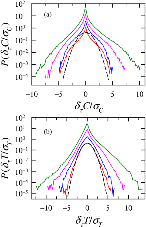
Figure 10: (Color online). PDFs of (a) concentration and (b) temperature increments normalized by their standard deviations for four time intervals $\tau/t_{B}=0.05$, 0.15, 1, and 10, from top to bottom. The curves have been shifted vertically for clarity and the black dashed curve indicates a Gaussian distribution of variance 1.

We have seen in Sec. III.1 that the right tail of concentration PDF, which describes the distribution of the mixed fluorescence dye, has a decreasing exponential shape. An exponential distribution near the tail means higher probability of rare events, i.e. intermittency, in comparison with the Gaussian distribution. The small-scale intermittency of concentration fluctuations can be characterized by the distributions of their increments over different scales. Figure 10(a) shows the measured PDFs of the concentration increments $\delta_{\tau}C(t)$ for four different time lags $\tau$, with $\tau$ = $0.05t_{B}$ (close to the dissipative scale), $0.15t_{B}$, $t_{B}$ (Bolgiano scale), and 10$t_{B}$ ($\sim t_{0}/4$), from top to bottom. The PDFs have been normalized by their own standard deviations $\sigma_{C}=\langle(\delta_{\tau}C)^{2}\rangle^{1/2}$ and shifted vertically for clarity. The dashed line in the figure represents a Gaussian distribution of variance 1 for reference. Three features are worthy of note: (i) all PDFs are strongly non-Gaussian from the smallest time interval to lags of the order of the large scale; (ii) all PDFs are clearly not self-similar, indicating strong intermittency; (iii) there is a slight asymmetry of the PDFs’ tails, especially for small time lags, reflecting the well-known property of small-scale persistence of anisotropy, i.e. ramp-cliff structures Sreenivasan (1991); Shraiman and Siggia (2000); Warhaft (2000).

The distributions of the normalized temperature increments $\delta_{\tau}T/\sigma_{T}$ ($\sigma_{T}=\langle(\delta_{\tau}T)^{2}\rangle^{1/2}$) for the same values of $\tau$ as those for the concentration are also examined, and are plotted in Fig. 10(b). The small-scale persistence of anisotropy can also be found for the active scalar increments from their asymmetric distributions at small time lags. This asymmetry can be linked to the sharp fronts of coherent structures in turbulent thermal convection, i.e. thermal plumes Zhou and Xia (2002). Another notable feature is that as time lags increase towards the large time scale the shapes of the PDFs evolve from approximately exponential tails to nearly Gaussian-like distribution, reflecting strong intermittency as well.

When comparing the PDFs of concentration and temperature increments, two features are remarkable: (i) The PDFs of temperature increments at small scales [the top two curves in Fig. 10(b)] are more asymmetric than those of concentration increments at the corresponding scales, suggesting that the mixing of temperature are more anisotropic than those of concentration. (ii) Qualitatively, Fig. 10 shows that the PDFs of temperature increments change from non-Gaussian in small scales to near Gaussian in large scales, whereas, those of concentration increments remain non-Gaussian for all scales investigated. In this sense, it suggests that the shapes of the concentration increments’ PDFs are less dissimilar among themselves than those of the temperature increments’ PDFs as time lags $\tau$ increase towards the large time scale, and hence the passive scalar is less intermittent than the active one Gasteuil et-al. (2007), which can also be quantified by the flatness discussed below.

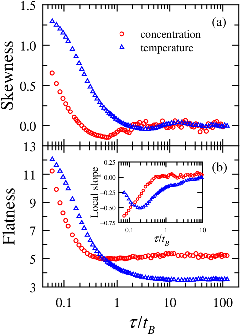
Figure 11: (Color online). (a) Skewness and (b) flatness of the concentration (red circles) and temperature (blue triangles) increments as functions of $\tau/t_{B}$. Inset of (b): the local slopes, $\chi^{X}(\tau/t_{B})=d\log{(F_{X}(\tau/t_{B}))}/d\log{(\tau/t_{B})}$, as functions of $\tau/t_{B}$.

To quantitatively characterize the anisotropic effects of the small-scale mixing of the two scalars, we study the skewness of their increments, i.e.,

$$S_{X}(\tau)=\langle(\delta_{\tau}X)^{3}\rangle/\langle(\delta_{\tau}X)^{2}\rangle^{3/2}.$$ (11)

where $\delta_{\tau}X(t)=X(t+\tau)-X(t)$ with $X=C$ for concentration and $X=T$ for temperature. The skewness is a global measure of asymmetry. By definition, the skewness of a symmetric-distributed quantity is 0. Figure 11(a) shows the measured skewness for the concentration and temperature increments. One sees that both $S_{C}(\tau)$ and $S_{T}(\tau)$ decrease with time lags for small $\tau$. $S_{C}(\tau)$ reaches its minimum value around $\tau\simeq 0.7t_{B}$ and then increases a little, whereas, $S_{T}(\tau)$ decreases almost monotonically to the zero value. For $\tau\lesssim t_{B}$, both temperature and concentration behave as passive scalars but one finds $|S_{T}(\tau)|>|S_{C}(\tau)|$, suggesting that the mixing of temperature are more anisotropic than those of concentration. This is because the mixing of a passive scalar field becomes more isotropic with decreasing diffusivity Schumacher and Sreenivasan (2003) and from Table I we see that the thermal diffusivity $\kappa_{T}$ is about two orders of magnitude larger than molecular diffusivity $\kappa_{C}$ of the dye. For $\tau\gtrsim t_{B}$, both $S_{C}(\tau)$ and $S_{T}(\tau)$ fluctuate around 0, implying that the mixing of both scalar are isotropic above the buoyant scale. This is strange since buoyancy effects act on fluids along the vertical direction but do not induce anisotropy for both temperature and concentration.

We now examine more quantitatively the intermittency levels of the two scalar fields. In general, the deviations of scaling exponents of structure functions, $R^{X}_{p}(\tau)=\langle|\delta_{\tau}X|^{p}\rangle\sim\tau^{\xi^{X}_{p}}$, in the inertial range from those expected by the arguments of Kolmogorov Kolmogorov (1941a, b) or Bolgiano R. Bolgiano (1959) and Obukhov A.M. Obukhov (1959) can be used as a measure for the degree of intermittency. Unfortunately, above the Bolgiano time scale $t_{B}$, no discernible scaling for concentration is observed no matter whether structure functions are plotted directly against time lags in a log-log plot or indirectly using an extended self-similarity method Benzi et-al. (1993a, b). Here, we use the flatness of the temperature and concentration increments, defined as,

$$F_{X}(\tau)=\langle(\delta_{\tau}X)^{4}\rangle/\langle(\delta_{\tau}X)^{2}\rangle^{2}=R^{X}_{4}/(R^{X}_{2})^{2}\sim\tau^{\chi^{X}},$$ (12)

to characterize their levels of intermittency, where $\chi^{X}=\xi^{X}_{4}-2\xi^{X}_{2}$. The flatness is a characteristic measure of whether the data are peaked or flat relative to a Gaussian distribution and hence can be used as a relatively sensitive measure of intermittency. By definition, the flatness of a Gaussian-distributed quantity is 3. In addition, the local slope of the flatness for the temperature and concentration increments, defined as

$$\chi^{X}(\tau)=d\log{(F_{X}(\tau))/d\log{\tau}},$$ (13)

may also be used as a measure of self-similarity, since $\chi^{X}(\tau)=0$ within a certain range of scales for a quantity whose increments are scale-free within that range. Therefore, larger deviations of $\chi^{X}(\tau)$ from 0 reflects less self-similarity, i.e. more intermittent. Figure 11(b) shows the measured $F_{C}(\tau)$ and $F_{T}(\tau)$ plotted as functions of time lags $\tau$. One sees that both quantities decrease with increasing $\tau$ for small $\tau$ and cross at $\tau\simeq 0.5t_{B}$. For $\tau>10t_{B}$, $F_{T}(\tau)$ levels off to a value of about 3.5, which is very close to that of a Gaussian-distributed quantity, while $F_{C}(\tau)$ levels off at a value of 5 for $\tau>0.5t_{B}$. The local slopes of $F_{C}(\tau)$ and $F_{T}(\tau)$ are plotted as functions of $\tau$ in the inset of Fig. 11(b). Above $t_{B}$, although one finds that the value of $F_{T}(\tau)$ is smaller than that of $F_{C}(\tau)$, temperature possesses a higher level of intermittency. This is because $\chi^{C}(\tau)\simeq 0$, suggesting an approximate self-similar property, and $|\chi^{T}(\tau)|>|\chi^{C}(\tau)|$, i.e. the deviations of $\chi^{T}(\tau)$ from 0 are larger than those of $\chi^{C}(\tau)$. Recall that within such regime buoyancy is important and the temperature field is an active scalar. Therefore, our results presented here suggest that the active scalar has a higher level of intermittency than the passive scalar, at least in turbulent thermal convection. Below $t_{B}$, the situation is more complicated. For $0.15t_{B}\lesssim\tau\lesssim t_{B}$, $|\chi^{T}(\tau)|>|\chi^{C}(\tau)|$ is obtained, again suggesting that temperature possesses a higher level of intermittency within such regime. Whereas, for $\tau\lesssim 0.15t_{B}$, we have $|\chi^{T}(\tau)|<|\chi^{C}(\tau)|$, suggesting that concentration is more intermittent for such regime. Note that this regime is close to the dissipative scale, but we don’t understand the mechanism that caused such result.

III.5 Cross-correlation between the concentration and temperature fluctuations

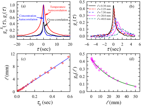
Figure 12: (Color online). (a) Autocorrelation functions $g_{a}^{T}(\tau)$ (red line), $g_{a}^{C}(\tau)$ (blue line) and cross-correlation function $g_{c}(\tau)$ (black line). The separation between the laser beam and the temperature probe is $\ell=0.375$ mm. (b) Cross-correlation functions $g_{c}(\tau)$ for five different separations $\ell$. (c) The separation $\ell$ vs the position of the measured correlation peak $\tau_{0}$. The solid line shows the fitting linear function $\ell=\bar{u}\tau_{0}$ with $\bar{u}=18.4$ mm/s. (d) The measured correlation amplitude $g_{0}(\ell)$ as a function of the separation $\ell$. The solid curve shows the fitting exponential function $g_{0}(\ell)=0.429e^{\displaystyle{-\ell/\xi}}$, with $\xi=27.3$ mm.

Figure 12(a) shows the measured auto-correlation functions,

$$g_{a}^{X}(\tau)=\frac{\displaystyle{\langle\delta X(t)\delta X(t+\tau)\rangle}}{\displaystyle{X_{rms}^{2}}},$$ (14)

for temperature ($X=T$) and concentration ($X=C$), respectively, and their cross-correlation function

$$g_{c}(\tau)=\frac{\displaystyle{\langle\delta C(t)\delta T(t+\tau)\rangle}}{\displaystyle{C_{rms}T_{rms}}}$$ (15)

as functions of time lag $\tau$, where $\delta X(t)=X(t)-\langle X(t)\rangle$. One sees that all three functions have a shape similar to each other, but the full width at half maximum (FWHM) of their peaks are different. The FWHMs of the temperature and concentration fluctuations are $W_{T}\simeq 3.7s$ and $W_{C}\simeq 0.5s$, respectively, and the FWHM of their cross-correlation is $W_{TC}\simeq 2.2s$, which is about the average of $W_{T}$ and $W_{C}$. One half of the FWHM of the correlation functions, $W_{T}/2$ ($W_{C}/2$), provides information about the transient time for the temperature (concentration) fluctuations of a certain size passing through the temperature (concentration) probe with a certain speed, and thus one can obtain the coherent length of the temperature (concentration) fluctuations from the FWHM and the advected speed. Since both scalars are transported by the same velocity field and the relation $W_{T}>W_{C}$ is obtained, we conclude that the coherent length of the active scalar, i.e. the size of thermal plumes, is larger than that of the passive scalar, i.e. the width of the cliff structures of the concentration field Sreenivasan (1991); Shraiman and Siggia (2000); Warhaft (2000); Moisy et-al. (2001), which is probably due to the larger value of the thermal diffusivity.

Figure 12(b) shows the measured concentration-temperature cross-correlation functions for five different sparation $\ell$. It is found that the measured $g(\tau)$ all have a single peak $g_{0}$ as concentration and temperature are both advected by the same velocity field. However, the peak position $\tau_{0}$ for different separation $\ell$ are not the same. The bigger $\ell$ is, the larger $\tau_{0}$ becomes. How the measured $\tau_{0}$ varies with the separation $\ell$ is plotted in Fig. 12(c). It can be clearly seen that $\ell$ increases with increasing $\tau_{0}$, and the increasing manner may be described by a simple linear function

$$\ell=\bar{u}\tau_{0},\mbox{\ \ }\bar{u}=18.4\mbox{\ mm/s}$$ (16)

The solid line in Fig. 12(c) shows the fitting linear equation (16). The slope $\bar{u}=18.4$ mm/s, describing the mean velocity with which the temperature and concentration fluctuations pass through the measuring points. Fig. 12(d) shows the relationship between the obtained $g_{0}$ and the separation $\ell$. It is clearly shown that $g_{0}(\ell)$ decreases with increasing $\ell$, and the decay may be described by a simple exponential function

$$g_{0}(\ell)=0.429e^{\displaystyle{-\ell/\xi}},\mbox{\ \ }\xi=27.3\mbox{\ mm}$$ (17)

The solid curve in Fig. 12(d) shows the fitting equation (17). A similar correlation length was also obtained in velocity-temperature cross-correlation functions in a cylindrical cell Shang et-al. (2004).

IV Summary and conclusion

To summarize, we have carried out a comparative study on local mixing of active and passive scalars in turbulent thermal convection. The statistical properties of local temperature are experimentally compared with those of local concentration. It is found that, although transported by the same turbulent flow field, the fluctuations of the two scalars are distributed differently: a decreasing exponential tail is found for the fluctuating concentration, while Gaussian-like tails for the fluctuating temperature. It is also shown that the temperature increments exhibit a positive and large correlation with the concentration increments above the Bolgiano time scale $t_{B}$; whereas this correlation decays with decreasing time lags $\tau$ for $\tau\lesssim t_{B}$. This reflects the fact that there is a certain buoyant scale in turbulent RBC, above which the buoyancy effects are important. Above $t_{B}$, temperature is active and the mixing of both scalars are isotropic even though buoyancy acts on the fluid in the vertical direction. While temperature fluctuations are found to be more intermittent than concentration fluctuations, suggesting that the active scalar possesses a higher level of intermittency in turbulent thermal convection. Below $t_{B}$, temperature is passive but its mixing are more anisotropic than those of concentration, reflecting the fact that its diffusivity ($\kappa_{T}$) is larger than that of concentration ($\kappa_{C}$). It is further found, from the simultaneous measurements of temperature and concentration, that the two scalars have similar autocorrelation functions and there is a strong and positive correlation between them. Future investigations will be focused on statistical and geometric features of the passive scalar field for varying Ra.