A New two-dimensional Second Order Non-oscillatory Central Scheme Applied to multiphase flows in heterogeneous porous media

¹ State University of Rio de Janeiro, Nova Friburgo, RJ 28630-050, Brazil.

² University of Wyoming, Laramie, WY 82071-3036, U.S.A.

Abstract

We are concerned with central differencing schemes for solving scalar hyperbolic conservation laws. We compare the Kurganov-Tadmor (KT) two-dimensional (Kurganov and Tadmor, 2000) second order semi-discrete central scheme in dimension by dimension formulation with a new two-dimensional approach introduced here and applied in numerical simulations for two-phase, two-dimensional flows in heterogeneous formations. This semi-discrete central scheme is based on the ideas of Rusanov’s method (Rusanov (1961)) using a more precise information about the local speeds of wave propagation computed at each Riemann Problem in two-space dimensions. We find the KT dimension by dimension has a much simpler mathematical description than the genuinely two-dimensional one with a little more numerical diffusion, particularly in the presence of viscous fingers. Unfortunately, as one can see in Abreu et al. (2007), the KT with the dimension by dimension approach might produce incorrect boundary behavior in a typical geometry used in the study of porous media flows: the quarter of a five spot. This problem has been corrected by the authors with the new semi-discrete scheme proposed here. We conclude with numerical examples of two-dimensional, two-phase flow associated with two distinct flooding problems: a two-dimensional flow in a rectangular heterogeneous reservoir (called slab geometry) and a two-dimensional flow in a 5-spot geometry homogeneous reservoir.

1. INTRODUCTION

We consider a model for two-phase flow, immiscible and incompressible displacement in heterogeneous porous media. The highly nonlinear governing equations are of very practical importance in petroleum engineering (Peaceman, 1977; Chavent and Jaffré, 1986) (see also (Furtado and Pereira, 2003) and the references therein for recent studies for the scale-up problem for such equations).

The conventional theoretical description of two-phase flow in a porous medium, in the limit of vanishing capillary pressure, is via Darcy’s law coupled to the Buckley-Leverett equation. The two phases will be referred to as water and oil, and indicated by the subscripts $w$ and $o$, respectively. We also assume that the two fluid phases saturate the pores. With no sources or sinks, and neglecting the effects of gravity these equations are (see Peaceman (Peaceman, 1977)):

$$\nabla\cdot{\bf v}=0,\quad{\bf v}=-\lambda(s)K({\bf x})\nabla p,$$ (1)

$$\frac{\partial s}{\partial t}+\nabla\cdot(f(s){\bf v})=0.$$ (2)

Here, ${\bf v}$ is the total seepage velocity, $s$ is the water saturation, $K({\bf x})$ is the absolute permeability, and $p$ is the pressure. The constant porosity has been scaled out by a change of the time variable. The constitutive functions $\lambda(s)$ and $f(s)$ represent the total mobility and the fractional flow of water, respectively.

We are concerned with numerical schemes for solving scalar hyperbolic conservation laws arising in the simulation of multiphase flows in multidimensional heterogeneous porous media. These schemes are non-oscillatory and enjoy the main advantage of Godunov-type central schemes: simplicity, i.e., they employ neither characteristic decomposition nor approximate Riemann solvers. This makes them universal methods that can be applied to a wide variety of physical problems, including hyperbolic systems of conservation laws. The two main classes of Godunov methods are upwind and central schemes.

The Lax-Friedrichs (LxF) scheme (Lax, 1954) is the canonical first order central scheme, which is the forerunner of all central differencing schemes. It is a non-oscillatory scheme based on piecewise constant approximate solution and it also enjoys simplicity. Unfortunately the excessive numerical dissipation in the LxF recipe (of order ${\mathcal{O}}(\Delta X^{2}/\Delta t)$) yields a poor resolution, which seems to have delayed the development of high resolution central schemes when compared with the earlier developments of the high resolution upwind methods. Only in 1990 a second order generalization to the LxF scheme was introduced in (Nessyahu and Tadmor, 1990). They used a staggered form of the LxF scheme and replaced the first order piecewise constant solution with a van Leer’s MUSCL-type piecewise linear second order approximation (Van Leer, 1979). The numerical dissipation present in this new central scheme has an amplitude of order ${\mathcal{O}}({\Delta X}^{4}/\Delta t)$. (see (Abreu et al., 2004c), (Abreu et al., 2004b), (Abreu et al., 2004a), (Abreu et al., 2006), for recent studies in three phase flows using the Nessyahu and Tadmor (NT) central scheme). In spite of the good resolution obtained by the Nessyahu and Tadmor scheme, much higher than in the first order LxF scheme, there are still some difficulties with small time steps which arise, e.g. in multiphase flows in highly heterogeneous petroleum reservoirs or aquifers. To overcome this difficulty, we can use a semi-discrete formulation coupled with an appropriate ODE solver retaining simplicity and high resolution with lower numerical viscosity, proportional to the vanishing size of the time step $\Delta t$. Both LxF and NT schemes do not admit a semi-discrete form; see (Kurganov and Tadmor, 2000) for a detailed description of the one-dimensional Kurganov and Tadmor central scheme which is the first fully discrete Godunov-Type central scheme admitting a semi-discrete form.

We compare the Kurganov-Tadmor (KT) two-dimensional (Kurganov and Tadmor, 2000) second order semi-discrete central scheme in dimension by dimension formulation with a genuinely two-dimensional approach applied in numerical simulations for two-phase, two-dimensional flows in heterogeneous formations. We find the KT dimension by dimension has a much simpler mathematical description than the genuinely two-dimensional one adding only a little more diffusion, particularly in the presence of viscous fingers. Unfortunately, the KT with the dimension by dimension approach might produce incorrect boundary behavior in a typical geometry used in the study of porous media flows: the quarter of a five spot. These results are presented in (Abreu et al., 2007). This problem motivated the authors to develop a genuinely two-dimensional formulation which is then presented in section (2.2). Although a similar two-dimensional formulation was available in a early work (Kurganov and Petrova, 2001), ours was developed independently to deal with two-phase flows, immiscible and incompressible displacement in heterogeneous porous media. It shares the same general ideas with the work of Kurganov-Petrovna but differs in many technical details.

This paper is organized as follows. In Section 2 we introduce the model for two-phase flows, immiscible and incompressible displacement in heterogeneous porous media. In Section 2.2 we discuss the mathematical formulation for the KT central scheme in dimension by dimension approach and in a genuinely two-dimensional one. In Section 3 we will present some numerical results when we apply the KT central differencing scheme with both approaches mentioned above to porous media flows.

2. NUMERICAL APPROXIMATION OF TWO-PHASE FLOW

2.1. Operator splitting for two-phase flow.

An operator splitting technique is employed for the computational solution of the saturation equation (2) and the pressure equation (1) which are solved sequentially with distinct time steps. This method has proved to be computationally efficient in producing accurate numerical solutions for two-phase flow (Douglas et al., 1997).

Typically, for computational efficiency, larger time steps are used to compute the pressure (1). The splitting allows time steps used in the solution of the pressure-velocity equation that are longer than those allowed in the convection calculation  (2). Thus, we introduce two time steps: $\Delta t_{c}$ used to compute the solution of the hyperbolic problem, and $\Delta t_{p}$ used in the pressure-velocity calculation such that $\Delta t_{p}\geq\Delta t_{c}$. We remark that in practice, variable time steps are always useful, especially for the convection micro-steps subject dynamically to a $CFL$ condition.

For the global pressure solution (the pertinent elliptic equation), we use a (locally conservative) hybridized mixed finite element discretization equivalent to cell-centered finite differences (Douglas et al., 1997), which effectively treats the rapidly changing permeabilities that arise from stochastic geology and produces accurate velocity fields. The pressure and the Darcy velocity are approximated at times $t^{m}=m\Delta t_{p}$, $m=0,1,2,\dots$. The algebraic system resulting from the discretized equations can be solved by a preconditioned conjugate gradient procedure (PCG) or by a multi-grid procedure ((Douglas et al., 1997)).

We use high resolution numerical central scheme (see (Kurganov and Tadmor, 2000)) for solving the scalar hyperbolic conservation laws arising in the convection of the fluid phases in heterogeneous porous media for two-phase flows - we will discuss the application of these schemes for two-phase flows in Section 3. Theses methods can accurately resolve sharp fronts in the fluid saturations without introducing spurious oscillations or excessive numerical diffusion.

The saturation equation is approximated at times $t^{\kappa}_{m}=t^{m}+{\kappa}\Delta t_{c}$ for $t^{m}<{t^{\kappa}_{m}}\leq t^{m+1}$ that take into account the advective transport of water. We will write $t^{\kappa}$ to indicate the time step ${t^{\kappa}_{m}}$ and $t^{\kappa+1}$ to indicate ${t^{\kappa}_{m}}+\Delta t_{c}$.

A detailed description of the numerical method that we employ for the solution of Eqs. (1)-(2) can be found in Douglas et al. (1997) and references therein (see also Abreu et al. (2006, 2004c) and Abreu et al. (2008) for applications of the operator splitting technique for three phase flows that takes into account capillary pressure (diffusive effects)).

Remark: To simplify notation, we denote:

• NT1d for one-dimensional NT scheme;

• NT2d for two-dimensional NT scheme;

• KT1d for one-dimensional KT scheme;

• KTdxd for the KT scheme with dimension by dimension approach and

• SD2-2D for our two-dimensional approach.

2.2. TWO SPATIAL DIMENSIONS SECOND ORDER SEMI-DISCRETE CENTRAL SCHEME

In this section, we will develop a two-spatial dimension second order semi-discrete central scheme (SD2-2D) based on the ideas of Lax (1954); Rusanov (1961); Nessyahu and Tadmor (1990); Kurganov and Tadmor (2000) and Jiang and Tadmor (1998) which are then applied in numerical approximation of the scalar hyperbolic conservation law modeling the convective transport of the fluid phases in two-phase flows and its coupling with lowest order Raviart-Thomas (Raviart and Thomas, 1977) locally conservative mixed finite elements for the associated elliptic (velocity-pressure part) problem (See Raviart and Thomas (1977)). We summarize below the basic ideas of the construction of SD2$-$2D numerical scheme:

• The Lax-Friedrichs method in two-spatial dimensions LxF2D written in the REA algorithm setup (See Jiang and Tadmor (1998)) will be used to obtain the two dimensional Rusanov’s method SD1-2D. We follow the same procedures presented in Kurganov and Tadmor (2000) in one spatial dimension.

• The new SD2-2D numerical scheme will then be obtained as a second order generalization of the SD1-2D. This second order precision is achieved approximating the solution with piecewise linear functions.

2.3. The staggered non-uniform grid of the SD2-2D central scheme

We begin then extending the LxF2D to obtain the SD1-2D following the same procedures for one dimensional problems. First, we define the non-staggered and the staggered grids of retangular cells used in the LxF2D. The points $(x_{j},y_{k},t^{\kappa})$ are defined as follows.

$$x_{j} = j\cdot\Delta x,\qquad j=\ldots,-1,0,1,\ldots$$

$$y_{k} = k\cdot\Delta y,\qquad k=\ldots,-1,0,1,\ldots$$

$$t^{\kappa} = t^{m}+\kappa\cdot\Delta t_{c},\qquad\kappa=0,\ldots,i,$$

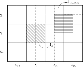
We denote the cells of the non-staggered grid by $I_{j,k}:=(x_{j-1/2},x_{j+1/2})\times(y_{k-1/2},y_{k+1/2})$. Its area $A_{j,k}\equiv\Delta x\cdot\Delta y=(x_{j+1/2}-x_{j-1/2})\cdot(y_{k+1/2}-y_{k-1/2})$. The time step of the convective equation (2) is $\Delta t_{c}=t^{\kappa+1}-t^{\kappa}$. The staggered grid is obtained moving the cells $\Delta x/2$ to the right and $\Delta y/2$ upward These staggered cells will be denoted by $I_{j+1/2,k+1/2}:=(x_{j},x_{j+1})\times(y_{k},y_{k+1})$. Its center is the point $(x_{j+1/2},y_{k+1/2})$, where $x_{j+1/2}=x_{j}+\Delta x/2$ and $y_{k+1/2}=y_{j}+\Delta y/2$. The Figure 1 illustrates the non-staggered and the staggered grids showing the cells $I_{j,k}$ e $I_{j+3/2,k+1/2}$ as examples of non-staggered and staggered cells, respectively.

Figure 1. The LxF2D uniform grid. The cells $I_{j,k}$ of the original non-staggered grid are limited by the solid lines and the cells $I_{j+3/2,k+1/2}$ of the staggered grid are limited by the dashed lines.

The scalar hyperbolic conservation law (2) can be written as

$$\frac{\partial s}{\partial t}+\frac{\partial}{\partial x}({{}^{x}\!v}f(s))+\frac{\partial}{\partial y}({{}^{y}\!v}f(s))=0,$$ (3)

where ${{}^{x}\!v}\equiv{{}^{x}\!v}(x,y,t)$ and ${{}^{y}\!v}\equiv{{}^{y}\!v}(x,y,t)$ denote the $x$ and $y$ components of the velocity field ${\bf v}$. The cell averages at time $t^{\kappa}$ are

$$\overline{S}^{\kappa}_{j,k}:=\overline{S}_{j,k}(t^{\kappa})\equiv\frac{1}{\Delta X\!\Delta Y}\displaystyle\int_{x_{j-\frac{1}{2}}}^{x_{j+\frac{1}{2}}}\displaystyle\int_{y_{k-\frac{1}{2}}}^{y_{k+\frac{1}{2}}}s(x,y,t^{\kappa})\,dxdy.$$ (4)

The solution $s(x,y,t^{\kappa})$ of the problem (2) at time $t^{\kappa}$ is approximated using piecewise-linear MUSCL-type interpolants (See Van Leer (1979)).

$$\widetilde{S}^{\kappa}_{j,k}(x,y)=\overline{S}^{\kappa}_{j,k}+(S_{x})^{\kappa}_{j,k}\cdot(x-x_{j})+(S_{y})^{\kappa}_{j,k}\cdot(y-y_{k}),$$ (5)

where $x_{j-1/2}\leq x\leq x_{j+1/2}$ e $y_{k-1/2}\leq y\leq y_{k+1/2}$. The second-order resolution is guaranteed if the so-called vector of numerical derivative $(S_{x})^{\kappa}_{j,k}$ and $(S_{y})^{\kappa}_{j,k}$ satisfy

$$(S_{x})^{\kappa}_{j,k} = \left.\frac{\partial s}{\partial x}\,\right|_{x=x_{j},y=y_{k},t=t^{\kappa}}+\mathcal{O}(\Delta X);$$ (6a)

$$(S_{y})^{\kappa}_{j,k} = \left.\frac{\partial s}{\partial y}\right|_{x=x_{j},y=y_{k},t=t^{\kappa}}+\mathcal{O}(\Delta Y),$$ (6b)

These numerical derivatives are computed using the MinMod limiter

$$(S_{x})^{\kappa}_{j,k} = \text{MM}\theta\frac{1}{\Delta x}\left\{\overline{S}^{\kappa}_{j-1,k},\overline{S}^{\kappa}_{j,k},\overline{S}^{\kappa}_{j+1,k}\right\}$$ (7a)

$$:= \text{MM}\left(\theta\frac{\Delta S^{\kappa}_{j+1/2,k}}{\Delta x},\frac{\Delta S^{\kappa}_{j-1/2,k}-\Delta S^{\kappa}_{j+1/2,k}}{2\Delta x},\theta\frac{\Delta S^{\kappa}_{j-1/2,k}}{\Delta x}\right);$$

$$(S_{y})^{\kappa}_{j,k} = \text{MM}\theta\frac{1}{\Delta y}\left\{\overline{S}^{\kappa}_{j,k-1},\overline{S}^{\kappa}_{j,k},\overline{S}^{\kappa}_{j,k+1}\right\}$$ (7b)

$$:= \text{MM}\left(\theta\frac{\Delta S^{\kappa}_{j,k+1/2}}{\Delta y},\frac{\Delta S^{\kappa}_{j,k-1/2}-\Delta S^{\kappa}_{j,k+1/2}}{2\Delta y},\theta\frac{\Delta S^{\kappa}_{j,k-1/2}}{\Delta y}\right).$$

Here $\Delta$ denotes the centered difference, $\Delta S^{\kappa}_{j+1/2,k}=\overline{S}^{\kappa}_{j+1,k}-\overline{S}^{\kappa}_{j,k}$ and the paramter $\theta\in[1,1.8]$ has been chosen in the optimal way in every numerical example with $\theta=1.8$ beeing the less dissipative limiter. The minmod limiter (7) guarantees the nonoscillatory property and the second-order accuracy. The reconstruction given by Equations (5)-(7) also retains conversation, i.e.,

$$\int_{I_{j,k}}\widetilde{S}^{\kappa}_{j,k}(x,y)\,dx\,dy=\overline{S}^{\kappa}_{j,k}.$$ (8)

Remark: We notice that if $(S_{x})^{\kappa}_{j,k}$ and $(S_{y})^{\kappa}_{j,k}$ are equal to zero, then we will get the first-order two-dimensional semi-discrete scheme SD1-2D. Otherwise, we will obtain the second-order two spatial dimensions semi-discrete central scheme SD2-2D.

We consider the model of hyperbolic conservation laws given by Equation (2) with cell averages as in (4) and the two-dimensional piecewise linear reconstruction defined in (5) and (6) with the conservative property (8). Our goal is to compute an approximated solution $S_{j,k}({t^{\kappa}_{m}}+\Delta t_{c})$ in the original grid at the next time step. To this end, we apply the Godunov’s algorithm REA. To solve this problem, we integrate the conservation law over some control volumes that we need to specify.

Constructing the staggered nonuniform grid: Kurganov and Tadmor developed the KT1D scheme along the lines of NT1D (See (Kurganov and Tadmor, 2000)). The nonuniform staggered grid in the KT1D was constructed directly from the staggered uniform grid of NT1D with additional information on the local speeds of wave propagation. In a similar way the nonuniform staggered grid in the SD2-2D scheme is defined from the uniform staggered grid of the NT2D scheme as follows.

$(1)$ We set $C_{j,k}=[x_{j-1/2},x_{j+1/2}]\times[y_{k-1/2},y_{k+1/2}]$ to denote the cells of the original non-staggered grid; $C_{j+1/2,k+1/2}=[x_{j},x_{j+1}]\times[y_{k},y_{k+1}]$ to denote the cells of the uniform staggered grid. We start with a piecewise constant approximated solution $\bar{S}^{\kappa}_{j,k}$ over the original cells $C_{j,k}$.

$(2)$ Next, we move to the staggered uniform grid with cells given by $C_{j+1/2,k+1/2}$.

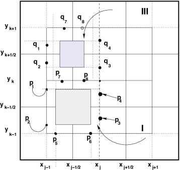
$(3)$ The NT2D scheme computes four averaged solutions at time step ${t^{\kappa}_{m}}+\Delta t_{c}$ (See the hachured regions in Figure 2 corresponding to the cells $C_{j-1/2,k-1/2}$, $C_{j+1/2,k-1/2}$, $C_{j-1/2,k+1/2}$ and $C_{j+1/2,k+1/2}$ on the staggered grid). These averaged staggered solution are then properly projected back onto the original non-staggered grid to obtain the desired solution (See Jiang and Tadmor (1998)).

Repeating the same ideias presented by Rusanov in his modification of Lax-Friedrichs’ method, we compute the local speed of propragation at each Riemann Problem. These local speeds define new non-uniform cells where the evolution step will take place.

Computing the local speed of propagation: we begin with the cell $C_{j-1/2,k-1/2}$ to find the local speeds at the following Riemann Problems:

1. Y direction:

   1. $$\left\{\begin{array}[]{ll}\overline{S}^{\kappa}_{j-1,k-1},&x_{j-3/2}\leq x\leq x_{j-1/2},\quad y_{k-3/2}\leq y\leq y_{k-1/2}\\ \overline{S}^{\kappa}_{j-1,k},&x_{j-3/2}\leq x\leq x_{j-1/2},\quad y_{k-1/2}\leq y\leq y_{k+1/2}.\end{array}\right.$$

      The local speed $a^{y}_{j-1,k-1/2}$ defines the following points:

      $$p_{1}=(x_{j-1},\,y_{k-1/2}-a^{y}_{j-1,k-1/2}{\Delta t_{c}}),$$

      $$p_{2}=(x_{j-1},\,y_{k-1/2}+a^{y}_{j-1,k-1/2}{\Delta t_{c}})$$

      sketched in Figure 2. We denote the distance between them by $\Delta y_{j-1,k-1/2}:=2a^{y}_{j-1,k-1/2}{\Delta t_{c}}$.

   2. $$\left\{\begin{array}[]{ll}\overline{S}^{\kappa}_{j,k-1},&x_{j-1/2}\leq x\leq x_{j+1/2},\quad y_{k-3/2}\leq y\leq y_{k-1/2}\\ \overline{S}^{\kappa}_{j,k},&x_{j-1/2}\leq x\leq x_{j+1/2},\quad y_{k-1/2}\leq y\leq y_{k+1/2}.\end{array}\right.$$

      The local speed $a^{y}_{j,k-1/2}$ defines the points

      $$p_{3}=(x_{j},\,y_{k-1/2}-a^{y}_{j,k-1/2}{\Delta t_{c}}),$$

      $$p_{4}=(x_{j},\,y_{k-1/2}+a^{y}_{j,k-1/2}{\Delta t_{c}})$$

      shown in Figure 2 and the distance between them is $\Delta y_{j,k-1/2}=2a^{y}_{j,k-1/2}{\Delta t_{c}}$.

2. X direction:

   1. $$\left\{\begin{array}[]{ll}\overline{S}^{\kappa}_{j-1,k-1},&x_{j-3/2}\leq x\leq x_{j-1/2},\quad y_{k-3/2}\leq y\leq y_{k-1/2}\\ \overline{S}^{\kappa}_{j,k-1},&x_{j-1/2}\leq x\leq x_{j+1/2},\quad y_{k-3/2}\leq y\leq y_{k-1/2}.\end{array}\right.$$

      The local speed $a^{x}_{j-1/2,k-1}$ defines the points

      $$p_{5}=(x_{j-1/2}-a^{x}_{j-1/2,k-1}{\Delta t_{c}},\,y_{k-1}),$$

      $$p_{6}=(x_{j-1/2}+a^{x}_{j-1/2,k-1}{\Delta t_{c}},\,y_{k-1})$$

      also shown in 2 and $\Delta x_{j-1/2,k-1}=2a^{x}_{j-1/2,k-1}{\Delta t_{c}}$ is the distance between them.

   2. $$\left\{\begin{array}[]{ll}\overline{S}^{\kappa}_{j-1,k},&x_{j-3/2}\leq x\leq x_{j-1/2},\quad y_{k-1/2}\leq y\leq y_{k+1/2}\\ \overline{S}^{\kappa}_{j,k},&x_{j-1/2}\leq x\leq x_{j+1/2},\quad y_{k-1/2}\leq y\leq y_{k+1/2}.\end{array}\right.$$

      The local speed $a^{x}_{j-1/2,k}$ defines the points

      $$p_{7}=(x_{j-1/2}-a^{x}_{j-1/2,k}{\Delta t_{c}},\,y_{k}),$$

      $$p_{8}=(x_{j-1/2}+a^{x}_{j-1/2,k}{\Delta t_{c}},y_{k})$$

      shown in Figure 2 and $\Delta X_{j-1/2,k}=2a^{x}_{j-1/2,k}{\Delta t_{c}}$ denotes the distance between them.

Given these four local speed of wave propagation $a^{y}_{j-1,k-1/2}$, $a^{y}_{j,k-1/2}$, $a^{x}_{j-1/2,k-1}$ e $a^{x}_{j-1/2,k}$, we can define the Region I (also represented by $R_{j-1/2,k-1/2}$) as follows:

• Region I:

  $$R_{j-1/2,k-1/2} := [x_{j-1/2}-b^{x}_{j-1/2,k-1/2}{\Delta t_{c}},\,x_{j-1/2}+b^{x}_{j-1/2,k-1/2}{\Delta t_{c}}]\times$$

  $$[y_{k-1/2}-b^{y}_{j-1/2,k-1/2}{\Delta t_{c}},\,y_{k-1/2}+b^{y}_{j-1/2,k-1/2}{\Delta t_{c}}]$$

  where $$b^{x}_{j-1/2,k-1/2}:=\max\{a^{x}_{j-1/2,k},a^{x}_{j-1/2,k-1}\}\hskip 8.5359pt\mbox{e}\hskip 8.5359pt$$

  $$b^{y}_{j-1/2,k-1/2}:=\max\{a^{y}_{j,k-1/2},a^{y}_{j-1,k-1/2}\}.$$

Figure 3 shows the new cell $R_{j-1/2,k-1/2}$ of the new staggered non-uniform grid.

Figure 2. SD2-2D: the construction of the two-dimensional grid

We repeat the same procedures with the cell $C_{j-1/2,k+1/2}$ to define the Region III in terms of the local speed of propagation $a^{y}_{j-1,k+1/2}$, $a^{y}_{j,k+1/2}$, $a^{x}_{j-1/2,k+1}$ e $a^{x}_{j-1/2,k}$. These local speeds determine analogously the points $q_{1}$ a $q_{8}$ sketched in Figure 3 and define the new Region III:

• Region III:

  $$R_{j-1/2,k+1/2} := [x_{j-1/2}-b^{x}_{j-1/2,k+1/2}{\Delta t_{c}},\,x_{j-1/2}+b^{x}_{j-1/2,k+1/2}{\Delta t_{c}}]\times$$

  $$[y_{k+1/2}-b^{y}_{j-1/2,k+1/2}{\Delta t_{c}},\,y_{k+1/2}+b^{y}_{j-1/2,k+1/2}{\Delta t_{c}}]$$

  where $$b^{x}_{j-1/2,k+1/2}:=\max\{a^{x}_{j-1/2,k},a^{x}_{j-1/2,k+1}\}\hskip 8.5359pt\mbox{and}\hskip 8.5359pt$$

  $$b^{y}_{j-1/2,k+1/2}:=\max\{a^{y}_{j,k+1/2},a^{y}_{j-1,k+1/2}\}.$$

Figure 3. Regions I and III

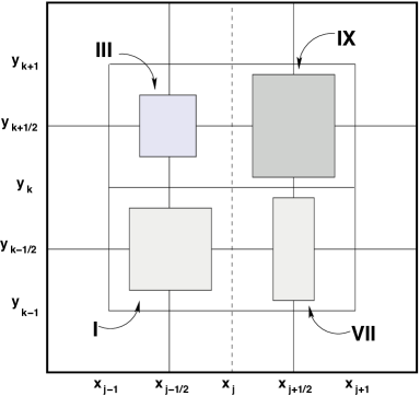
Following these same procedures with the staggered cells $C_{j+1/2,k-1/2}$ and $C_{j+1/2,k+1/2}$ we define Regions VII and IX shown in Figure 4. We will denote by Group A the set of Regions I, III, VII and IX.

Figure 4. Regions I, III, VII and IX

Finally, to finish the construction of the new non-uniform staggered grid, we need to define:

• Four cells which lie in the empty spaces between the regions of Group A. This new set will be denoted by Group B.

• A central region where the solution is smooth.

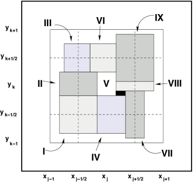
The definitions of the cells of Group B will determine the central region. This central region will not be a rectangle, but a set of retangles. There are many ways to define the cells of Group B. Our definition will be as follows (See Figura 5):

Figure 5. SD2-2D: The two dimensional semi-discrete central scheme SD2-2D: construction of the non-uniform staggered grid.

• Region II:

  $$R_{j-1/2,k} := [x_{j-1/2}-c^{x}_{j-1/2,k}{\Delta t_{c}},\,x_{j-1/2}+c^{x}_{j-1/2,k}{\Delta t_{c}}]\times$$

  $$[y_{k-1/2}+b^{y}_{j-1/2,k-1/2}{\Delta t_{c}},\,y_{k+1/2}-b^{y}_{j-1/2,k+1/2}{\Delta t_{c}}]$$

  $$\mbox{where}\quad c^{x}_{j-1/2,k}:=\max\{b^{x}_{j-1/2,k-1/2},b^{x}_{j-1/2,k+1/2}\}$$

The Regions VI and VIII can be obtained analogously As soon as the cells of Group A and B are determined, the central region is automatically defined:

• Region V:

  $$R_{j,k} := [x_{j-1/2}+c^{x}_{j-1/2,k}{\Delta t_{c}},\,x_{j+1/2}-c^{x}_{j+1/2,k}{\Delta t_{c}}]\times$$

  $$[y_{k-1/2}+d^{y}_{j,k-1/2}{\Delta t_{c}},\,y_{k+1/2}-d^{y}_{j,k+1/2}{\Delta t_{c}}].$$

We also would like to emphasize that our choice for these regions does not introduce more numerical diffusion. We will call BR the black rectangle that can be seen in Figure 5 and we notice that, by construction, its area is proportional to $(\Delta t_{c})^{2}$.

2.4. The new SD2-2D central scheme using Algorithm REA

After defining the new control volumes performed in the section above, we are now able to develop our new SD2-2D central scheme following the REA algorithm.

Reconstruction step: We suppose that we know an approximated solution constant in each cell at time step $t^{\kappa}$ as in Equation (4). This approximated solution is then reconstructed as a piecewise bilinear polinomial as defined in Equations (5) and (6). Evolution step: Let $D$ represents one of the nine regions defined above $R_{j\pm 1/2,k\pm 1/2}$, $R_{j,k\pm 1/2}$, $R_{j\pm 1/2,k}$, the central region $R_{j,k}$ or the black rectangle BR. We will denote by $D^{+}$ the part of region $D$ inside the non-staggered cell $I_{j,k}$ and by $D^{-}$, the part of region $D$ outside the cell $I_{j,k}$.

We integrate the conservation law (2) in the control volumes $D\times[{t^{\kappa}_{m}},{t^{\kappa}_{m}}+{\Delta t_{c}}]$ to obtain an approximate averaged solution $\bar{w}^{\kappa+1}(D)$ at the next time step, in each cell $D$ of the staggered non-uniform grid.

Projection step: These averaged solutions $\overline{w}^{\kappa+1}(D)$ are then reconstructed as piecewise bilinear polynomials $\widetilde{w}^{\kappa+1}(x,y)$ in each of the ten regions $D$. These new reconstructions are then projected back onto the original grid of uniform non-staggered cells,

$$\overline{S}^{\kappa+1}_{j,k}:=\frac{1}{\Delta x\,\Delta y}\int_{\bigcup D}\widetilde{w}^{\kappa+1}(x,y)\,dx\,dy.$$ (9)

The new reconstructions $\widetilde{w}^{\kappa+1}(x,y)$ are defined analogously as in Equation (5). For instance, for Region $R_{j+1/2,k}$,

$${\widetilde{w}^{\kappa+1}_{j+1/2,k}}(x,y)=\overline{w}^{\kappa+1}_{j+1/2,k}+(w_{x})^{\kappa+1}_{j+1/2,k}(x-x_{j+1/2})+ (w_{y})^{\kappa+1}_{j+1/2,k}(y-y_{k}),$$ (10)

$$(x,y)\in R_{j+1/2,k}.$$

The numerical derivatives $(w_{x})^{\kappa+1}_{j+1/2,k}$ and $(w_{y})^{\kappa+1}_{j+1/2,k}$ satisfy the conditions

$$(w_{x})^{\kappa+1}_{j+1/2,k} = \left.\frac{\partial w}{\partial x}\,\right|_{(x_{j+1/2},y_{k},t^{\kappa+1})}+\mathcal{O}(\Delta x);$$ (11)

$$(w_{y})^{\kappa+1}_{j+1/2,k} = \left.\frac{\partial w}{\partial y}\,\right|_{(x_{j+1/2},y_{k},t^{\kappa+1})}+\mathcal{O}(\Delta y);$$ (12)

in order to guarantee the second order approximation. Also, the reconstruction $\widetilde{w}^{\kappa+1}_{j+1/2,k}(x,y)$ retains the conservation property (8). We remark that this is a theoretical step and it will not be necessary to compute these numerical derivatives in the final semi-discrete formulation.

This completes the construction of our totally discrete central scheme in a rectangular grid. It is very laborious to write a totally discrete version of this central scheme. Instead, we will proceed directly to our semi-discrete formulation. In order to to this, we compute the following limit when ${\Delta t_{c}}\rightarrow 0$,

$$\lim_{{\Delta t_{c}}{\rightarrow}0} \frac{\overline{S}_{j,k}(t+{\Delta t_{c}})-\overline{S}_{j,k}(t)}{{\Delta t_{c}}}=\frac{d}{dt}\overline{S}_{j,k}(t)=$$

$$=\lim_{{\Delta t_{c}}{\rightarrow}0}\frac{1}{{\Delta t_{c}}}\cdot\frac{1}{\Delta x\,\Delta y}\left\{\sum_{p=j\pm 1/2}\int_{R^{+}_{p,k+1/2}}\widetilde{w}^{\kappa+1}_{p,k+1/2}(x,y)\right.$$

$$\left.+\sum_{p=j\pm 1/2}\int_{R^{+}_{p,k-1/2}}\widetilde{w}^{\kappa+1}_{p,k-1/2}(x,y)+\sum_{p=j\pm 1/2}\int_{R^{+}_{p,k}}\widetilde{w}^{\kappa+1}_{p,k}(x,y)\,dx\,dy\right.$$

$$\left.+\sum_{q=k\pm 1/2}\int_{R^{+}_{j,q}}\widetilde{w}^{\kappa+1}_{j,q}(x,y)\,dx\,dy+\int_{R_{j,k}}\widetilde{w}^{\kappa+1}_{j,k}(x,y)\,dx\,dy\right.$$

$$\left.+\int_{RP}\widetilde{w}^{\kappa+1}_{j+1/2,k-1/2}(x,y)dxdy-(\Delta x\,\Delta y)\overline{S}_{j,k}(t)\right\}$$ (13)

The conservation property of the reconstructions $\widetilde{w}^{\kappa+1}_{j,k}$ in he regions $D$ results

$$\int_{D}\widetilde{w}^{\kappa+1}(x,y)\,dx\,dy=|D|\cdot\overline{w}^{\kappa+1}(D),$$ (14)

where $\overline{w}^{\kappa+1}(D)$ is the averaged solution in region $D$. Note that, by reconstruction, the area of regions I, III, VII and IX are proportional to $({\Delta t_{c}})^{2}$, that is,

$$\begin{array}[]{ll}\mbox{Region I: }&|R_{j-1/2,k-1/2}|=\mathcal{O}\big{(}({\Delta t_{c}})^{2}\big{)}\\ \mbox{Region III: }&|R_{j-1/2,k+1/2}|=\mathcal{O}\big{(}({\Delta t_{c}})^{2}\big{)}\\ \mbox{Region VII: }&|R_{j+1/2,k-1/2}|=\mathcal{O}\big{(}({\Delta t_{c}})^{2}\big{)}\\ \mbox{Region IX: }&|R_{j+1/2,k+1/2}|=\mathcal{O}\big{(}({\Delta t_{c}})^{2}\big{)}\\ \mbox{Region RP: }&|RP|=\mathcal{O}\big{(}({\Delta t_{c}})^{2}\big{)}\\ \end{array}$$

For example, considering Region IX, we conclude

$$\int_{R_{j+1/2,k+1/2}}\widetilde{w}^{\kappa+1}_{j+1/2,k+1/2}(x,y)\,dx\,dy=\mathcal{O}({\Delta t_{c}})^{2}$$

$$\hskip 85.35826pt\Rightarrow\lim_{{\Delta t_{c}}{\rightarrow}0}\frac{1}{{\Delta t_{c}}}\int_{R_{j+1/2,k+1/2}}\widetilde{w}^{\kappa+1}_{j+1/2,k+1/2}(x,y)\,dx\,dy=0;$$ (15)

Our goal is to obtain the semi-discrete formulation of this new central cheme. Therefore, the Equation (2.4) show that we do not need to computed the averaged soltions over the Regions I, III, VII and IX. Note that, by simetry, we only need to compute the solutions over the Regions VI, VIII, V and the Black Rectangle. For the Region $R_{j+1/2,k}$, we obtain:

$$\int_{R^{+}_{j+1/2,k}}\widetilde{w}^{\kappa+1}_{j+1/2,k}(x,y)dxdy=$$

$$=\int_{R^{+}_{j+1/2,k}}\Big{[}\bigg{(}\overline{w}^{\kappa+1}_{j+1/2,k}+(w_{x})^{\kappa+1}_{j+1/2,k}\cdot(x-x_{j+1/2})+(w_{y})^{\kappa+1}_{j+1/2,k}\cdot(y-y_{k})\bigg{)}\Big{]}dxdy$$

$$=\overline{w}^{\kappa+1}_{j+1/2,k}\cdot|R^{+}_{j+1/2,k}|+\mathcal{O}(({\Delta t_{c}})^{2}).$$ (16)

Analogously, we compute the averaged solution over Region $R^{+}_{j,k+1/2}$:

$$\int_{R^{+}_{j,k+1/2}}\widetilde{w}^{\kappa+1}_{j,k+1/2}(x,y)dxdy=\overline{w}^{\kappa+1}_{j,k+1/2}\cdot|R^{+}_{j,k+1/2}|+\mathcal{O}(({\Delta t_{c}})^{2}).$$ (17)

Note that the solution has no discontinuities inside $R_{j,k}$. So, it isn’t necessary to reconstruction as a piecewise bilinear polynomials. The averaged solution is

$$\int_{R_{j,k}}\widetilde{w}^{\kappa+1}_{j,k}(x,y)dxdy=\overline{w}^{\kappa+1}_{j,k}\cdot|R_{j,k}|.$$ (18)

Substituting the Equations (2.4), (2.4), (17) and (18) in Equation (2.4), we obtain:

$$\frac{d}{dt}\overline{S}_{j,k}(t)= \lim_{{\Delta t_{c}}{\rightarrow}0}\left\{\frac{c^{x}_{j-1/2,k}}{\Delta x}\overline{w}_{j-1/2,k}(t+{\Delta t_{c}})+\frac{c^{x}_{j+1/2,k}}{\Delta x}\overline{w}_{j+1/2,k}(t+{\Delta t_{c}})\right.$$

$$\left.+\frac{d^{y}_{j,k-1/2}}{\Delta y}\overline{w}_{j,k-1/2}(t+{\Delta t_{c}})+\frac{d^{y}_{j,k+1/2}}{\Delta Y}\overline{w}_{j,k+1/2}(t+{\Delta t_{c}})\right.$$

$$\left.-\left(\frac{d^{y}_{j,k+1/2}+d^{y}_{j,k-1/2}}{\Delta y}+\frac{c^{x}_{j+1/2,k}+c^{x}_{j-1/2,k}}{\Delta x}\right)\cdot\overline{w}_{j,k}(t+{\Delta t_{c}})\right.$$

$$\left.+\left(\frac{1}{{\Delta t_{c}}}\overline{w}_{j,k}(t+{\Delta t_{c}})-\frac{1}{{\Delta t_{c}}}\overline{S}_{j,k}(t+{\Delta t_{c}})\right)\right\}.$$ (19)

For the final formulation, we have to compute the averaged solution over the non-uniform staggered grid.

$$\overline{w}^{\kappa+1}_{j+1/2,k},\overline{w}^{\kappa+1}_{j,k+1/2}\mbox{ e }\overline{w}^{\kappa+1}_{j,k},$$

To this end, we integrate the conservation law (LABEL:eq:sist2_cont) over the control volumes

$$R_{j+1/2,k}\times[{t^{\kappa}_{m}},{t^{\kappa}_{m}}+{\Delta t_{c}}],\quad R_{j,k+1/2}\times[{t^{\kappa}_{m}},{t^{\kappa}_{m}}+{\Delta t_{c}}]\quad\mbox{e}\quad R_{j,k}\times[{t^{\kappa}_{m}},{t^{\kappa}_{m}}+{\Delta t_{c}}],$$

respectively. Therefore,

$$w^{\kappa+1}_{j+1/2,k} =\frac{1}{|R_{j+1/2,k}|}\int_{R_{j+1/2,k}}s(x,y,t^{\kappa+1})\,dx\,dy$$

$$=\frac{1}{|R_{j+1/2,k}|}\int_{R_{j+1/2,k}}\widetilde{S}^{\kappa}(x,y)\,dx\,dy$$

$$-\frac{1}{|R_{j+1/2,k}|}\int_{R_{j+1/2,k}}\int_{t^{\kappa}}^{t^{\kappa+1}}\bigg{[}\frac{\partial}{\partial x}\bigg{(}{{}^{x}\!v}(x,y,\tau)\cdot f(s(x,y,\tau))\bigg{)}$$ (20)

$$\hskip 85.35826pt+\frac{\partial}{\partial y}\bigg{(}{{}^{y}\!v}(x,y,\tau)\cdot f(s(x,y,\tau))\bigg{)}\bigg{]}\,dx\,dyd\tau.$$

Let us denote the double integral by Int${}_{\widetilde{S}}$ and the flux integral by Int_f. The integral Int${}_{\widetilde{S}}$ is computed analytically.

$$\mbox{Int}_{\widetilde{S}}= \frac{1}{2}(\overline{S}^{\kappa}_{j,k}+\overline{S}^{\kappa}_{j+1,k})$$

$$+\frac{1}{4}\left[\Delta x-c^{x}_{j+1/2,k}{\Delta t_{c}}\right]\cdot\left[(S_{x})^{\kappa}_{j,k}-(S_{x})^{\kappa}_{j+1,k}\right]$$ (21)

$$+\frac{{\Delta t_{c}}}{4}\left[b^{y}_{j+1/2,k-1/2}-b^{y}_{j+1/2,k+1/2}\right]\cdot\left[(S_{y})^{\kappa}_{j,k}-(S_{y})^{\kappa}_{j+1,k}\right].$$

To compute the flux integral, Int_f, we first denote the limits of region $R_{j+1/2,k}$ as follows:

$$a:=x_{j+1/2}-c^{x}_{j+1/2,k}{\Delta t_{c}}$$

$$b:=x_{j+1/2}+c^{x}_{j+1/2,k}{\Delta t_{c}}$$

$$c:=y_{k+1/2}+b^{y}_{j+1/2,k-1/2}{\Delta t_{c}}$$

$$d:=y_{k+1/2}-b^{y}_{j+1/2,k+1/2}{\Delta t_{c}}$$

Using the Calculus Fundamental Theorem together with the trapezoid rule, we obtain

$$\mbox{Int}_{f} = \frac{1}{2\Delta x_{j+1/2,k}}\int_{t^{\kappa}}^{t^{\kappa+1}}\Big{[}{{}^{x}\!v}(b,d,\tau)\,f(s(b,d,\tau))-{{}^{x}\!v}(a,d,\tau)\,f(s(a,d,\tau))$$ (22)

$$+{{}^{x}\!v}(b,c,\tau)\,f(s(b,c,\tau))-{{}^{x}\!v}(a,c,\tau)\,f(s(a,c,\tau))\Big{]}\,d\tau$$

$$+\frac{1}{2\Delta y_{j+1/2,k}}\int_{t^{\kappa}}^{t^{\kappa+1}}\Big{[}{{}^{y}\!v}(b,d,\tau)\,f(s(b,d,\tau))-{{}^{y}\!v}(b,c,\tau)\,f(s(b,c,\tau))$$

$$+{{}^{y}\!v}(a,d,\tau)\,f(s(a,d,\tau))-{{}^{y}\!v}(a,c,\tau)\,f(s(a,c,\tau))\Big{]}\,d\tau$$

If the CFL condition

$$\max\left(\frac{{\Delta t_{c}}}{\Delta x}\max_{S}|{{}^{x}\!v}\,f^{\prime}(s)|,\frac{{\Delta t_{c}}}{\Delta y}\max_{S}|{{}^{y}\!v}\,f^{\prime}(s)|\right)<\frac{1}{2}$$ (23)

holds and since the functions ${{}^{x}\!v}\,f(s(x,y,\tau))$ and ${{}^{y}\!v}\,f(s(x,y,\tau))$ are computed away from the discontinuities then they are differential functions of $\tau$ and therefore, the time integral can be approximated using the middle point rule. Denoting $t^{\kappa+1/2}:=t+{\Delta t_{c}}/2$, we obtain:

$$\mbox{Int}_{f} = \displaystyle{\frac{1}{4c^{x}_{j+1/2,k}}\Big{[}{{}^{x}\!v}(b,d,t^{\kappa+1/2})\,f(S(b,d,t^{\kappa+1/2}))-{{}^{x}\!v}(a,d,t^{\kappa+1/2})\,f(S(a,d,t^{\kappa+1/2}))}$$ (24)

$$\displaystyle{+{{}^{x}\!v}(b,c,t^{\kappa+1/2})\,f(S(b,c,t^{\kappa+1/2}))-{{}^{x}\!v}(a,c,t^{\kappa+1/2})\,f(S(a,c,t^{\kappa+1/2}))\Big{]}\,d\tau}$$

$$\displaystyle{+\frac{\alpha_{Y}}{2-2\alpha_{Y}(b^{y}_{j+1/2,k+1/2}-b^{y}_{j+1/2,k-1/2})}}\cdot$$

$$\displaystyle{\Big{[}{{}^{y}\!v}(b,d,t^{\kappa+1/2})\,f(S(b,d,t^{\kappa+1/2}))-{{}^{y}\!v}(b,c,t^{\kappa+1/2})\,f(S(b,c,t^{\kappa+1/2}))}$$

$$\displaystyle{+{{}^{y}\!v}(a,d,t^{\kappa+1/2})\,f(S(a,d,t^{\kappa+1/2}))-{{}^{y}\!v}(a,c,t^{\kappa+1/2})\,f(S(a,c,t^{\kappa+1/2}))\Big{]}\,d\tau}$$

where $\alpha_{X}={\Delta t_{c}}/\Delta X$ and $\alpha_{Y}={\Delta t_{c}}/\Delta Y$.

The midpoint values are computed using the Taylor expansions and the conservation law (2). For instance,

$$\left\{\begin{array}[]{l}S(a,d,t^{\kappa+1/2}):=S(a,d,t)\\ \hskip 85.35826pt\displaystyle{-\frac{{\Delta t_{c}}}{2}\Big{(}{{}^{x}\!v}(a,d,t)\,f(S(a,d,t))\Big{)}_{x}}\displaystyle{-\frac{{\Delta t_{c}}}{2}\Big{(}{{}^{y}\!v}(a,d,t)\,f(S(a,d,t))\Big{)}_{y}}\\ \\ \displaystyle{S(a,d,t):=\overline{S}^{\kappa}_{j+1,k}-\Delta x\,(S_{x})^{\kappa}_{j+1,k}\Big{(}\frac{1}{2}-\alpha_{X}c^{x}_{j+1/2,k}\Big{)}}\displaystyle{-\Delta y\,(S_{y})^{\kappa}_{j+1,k}\Big{(}\frac{1}{2}-\alpha_{Y}b^{y}_{j+1/2,k+1/2}\Big{)}}.\end{array}\right.$$

As the time step ${\Delta t_{c}}$ goes to zero, the limit

$$\lim_{{\Delta t_{c}}{\rightarrow}0}S(a,d,t^{\kappa+1/2})=\overline{S}^{\kappa}_{j+1,k}-\frac{\Delta X}{2}\,(S_{x})^{\kappa}_{j+1,k}-\frac{\Delta Y}{2}\,(S_{y})^{\kappa}_{j+1,k}:=S^{++}_{j+1/2,k-1/2}.$$ (25)

These are called the intermediate values and their general form is

$$S^{\pm\pm}_{j+1/2,k+1/2} = \overline{S}^{\kappa}_{j+1/2\pm 1/2,k+1/2\pm 1/2}\pm\frac{\Delta X}{2}\,(S_{x})^{\kappa}_{j+1/2\pm 1/2,k+1/2\pm 1/2}(x_{j+1/2}-x_{j+1/2\pm 1/2})$$ (26)

$$\pm\frac{\Delta Y}{2}\,(S_{y})^{\kappa}_{j+1/2\pm 1/2,k+1/2\pm 1/2}(y_{k+1/2}-y_{k+1/2\pm 1/2})$$

We notice that the cell averages $w^{\kappa+1}_{j,k+1/2}$ and $w^{\kappa+1}_{j,k}$ are obtained analogously to (2.4). And also, $w^{\kappa+1}_{j-1/2,k}=w^{\kappa+1}_{j+1/2-1,k}$ e $w^{\kappa+1}_{j,k-1/2}=w^{\kappa+1}_{j,k+1/2-1}$.

Substituting all these cell averages in time step ${t^{\kappa}_{m}}+{\Delta t_{c}}$ into Equation (2.4) and computing the limit when ${\Delta t_{c}}{\rightarrow}0$, we obtain the second order central scheme in semi-discrete formulation:

$$\frac{d}{dt}\overline{S}_{jk}(t)=-\frac{H^{x}_{j+1/2,k}(t)-H^{x}_{j-1/2,k}(t)}{\Delta X}-\frac{H^{y}_{j,k+1/2}(t)-H^{y}_{j,k-1/2}(t)}{\Delta Y},$$ (27)

where the numerical fluxes are

$$H^{x}_{j+1/2,k}(t)= \frac{1}{4}\Big{\{}{{}^{x}\!v}_{j+1/2,k+1/2}(t)\Big{[}f(S^{+-}_{j+1/2,k+1/2}(t))+f(S^{--}_{j+1/2,k+1/2}(t))\Big{]}$$

$$+{{}^{x}\!v}_{j+1/2,k-1/2}(t)\Big{[}f(S^{++}_{j+1/2,k-1/2}(t))+f(S^{-+}_{j+1/2,k-1/2}(t))\Big{]}\Big{\}}$$

$$-\frac{c^{x}_{j+1/2,k}}{2}\Big{[}S^{+}_{j+1/2,k}(t)-S^{-}_{j+1/2,k}(t)\Big{]};$$ (28a)

$$H^{y}_{j,k+1/2}(t) =\frac{1}{4}\Big{\{}{{}^{y}\!v}_{j+1/2,k+1/2}(t)\Big{[}f(S^{-+}_{j+1/2,k+1/2}(t))+f(S^{--}_{j+1/2,k+1/2}(t))\Big{]}$$

$$+{{}^{y}\!v}_{j-1/2,k+1/2}(t)\Big{[}f(S^{++}_{j-1/2,k+1/2}(t))+f(S^{+-}_{j-1/2,k+1/2}(t))\Big{]}\Big{\}}$$

$$-\frac{d^{y}_{j,k+1/2}}{2}\Big{[}S^{+}_{j,k+1/2}(t)-S^{-}_{j,k+1/2}(t)\Big{]}.$$ (28b)

If the numerical derivatives are equal to zero then we obtain the two-dimensional Rusanov’s central scheme in semi-discrete formulation.

$$\mbox{{Rusa}}^{x}_{j+1/2,k}(t)= \frac{1}{4}\Big{\{}{{}^{x}\!v}_{j+1/2,k+1/2}(t)\Big{[}f(S_{j+1,k}(t))+f(S_{j,k}(t))\Big{]}$$

$$+{{}^{x}\!v}_{j+1/2,k-1/2}(t)\Big{[}f(S_{j+1,k}(t))+f(S_{j,k}(t))\Big{]}\Big{\}}$$

$$-\frac{c^{x}_{j+1/2,k}}{2}\Big{[}S_{j+1,k}(t)-S_{j,k}(t)\Big{]};$$ (29a)

$$\mbox{{Rusa}}^{y}_{j,k+1/2}(t)= \frac{1}{4}\Big{\{}{{}^{y}\!v}_{j+1/2,k+1/2}(t)\Big{[}f(S_{j,k+1}(t))+f(S_{j,k}(t))\Big{]}$$

$$+{{}^{y}\!v}_{j-1/2,k+1/2}(t)\Big{[}f(S_{j,k+1}(t))+f(S_{j,k}(t))\Big{]}\Big{\}}$$

$$-\frac{d^{y}_{j,k+1/2}}{2}\Big{[}S_{j,k+1}(t)-S_{j,k}(t)\Big{]}.$$ (29b)

This new two-dimensional semi-discrete central scheme with the numerical fluxes given by (28) or (29) comprises a system of ordinary differential equations. To solve this system, we use the explicit second order Runge-Kutta method.

2.5. The velocity field

Finally, to complete the description of the genuinely two-dimensional KT scheme, we have to define the velocity field. The velocity is defined at the vertices of the cells. We can not use directly the velocity field from the Raviart-Thomas space as we did in the dimension by dimension approach. Instead we will use a bilinear interpolation of it preserving the null divergence necessary for the incompressible flows. For instance, to compute the value of ${{}^{x}\!v}_{j+1/2,k+1/2}$ on the vertex $(x_{j+1/2},y_{k+1/2})$ at some time step $t^{m}$, we have to use all the four cells which share this vertex,

$${{}^{x}\!v}_{j+1/2,k+1/2} = \frac{1}{2}\Big{(}{{}^{x}\!v}_{j,k+1/2}+{{}^{x}\!v}_{j+1,k+1/2}\Big{)}$$

$$= \frac{1}{2}\Big{[}\frac{1}{2}\Big{(}{{}^{x}\!v}_{j,k}+{{}^{x}\!v}_{j,k+1}\Big{)}+\frac{1}{2}\Big{(}{{}^{x}\!v}_{j+1,k}+{{}^{x}\!v}_{j+1,k+1}\Big{)}\Big{]}$$

$$= +\frac{1}{2}\Big{[}\frac{1}{2}\Big{(}\frac{1}{2}(\vec{v_{r}}_{j+1/2,k}-\vec{v_{l}}_{j-1/2,k})$$

$$+\frac{1}{2}(\vec{v_{r}}_{j+1/2,k+1}-\vec{v_{l}}_{j-1/2,k+1}\Big{)}+\frac{1}{2}\Big{(}\frac{1}{2}(\vec{v_{r}}_{j+3/2,k}-\vec{v_{l}}_{j+1/2,k})+$$

$$\frac{1}{2}(\vec{v_{r}}_{j+3/2,k+1}-\vec{v_{l}}_{j+1/2,k+1})\Big{)}$$

$$= \frac{1}{8}\Big{(}\vec{v_{r}}_{j+1/2,k}-\vec{v_{l}}_{j-1/2,k}+\vec{v_{r}}_{j+1/2,k+1}-\vec{v_{l}}_{j-1/2,k+1}$$

$$+\vec{v_{r}}_{j+3/2,k}-\vec{v_{l}}_{j+1/2,k}+\vec{v_{r}}_{j+3/2,k+1}-\vec{v_{l}}_{j+1/2,k+1}\Big{)}$$

3. TWO-DIMENSIONAL NUMERICAL EXPERIMENTS

We present and compare the results for numerical simulations of two-dimensional, two-phase flow associated with two distinct flooding problems using the KT scheme with the dimension by dimension approach (KT dxd) and the genuinely two-dimensional formulation (SD2-2D). The first problem is a two-dimensional flow in a rectangular heterogeneous reservoir (called slab geometry) with $256$ m $\times$ $64$ m in size, and the second is a two-dimensional flow in a 5-spot geometry homogeneous reservoir having $64$ m $\times$ $64$ m.

In the 5-spot geometry homogeneous reservoir simulation we used two distinct uniform five-spot well configurations intended to illustrate different flow patterns, with parallel and diagonal grid orientations, and boundary behavior.

In all simulations the reservoir contains initially $79\%$ of oil and $21\%$ of water. Water is injected at a constant rate of $0.2$ pore volumes every year.

The fractional volumetric flow, the total mobility, and the relative permeabilities are assumed to be:

$$f(s)=\frac{k_{rw}(s)/\mu_{w}}{\lambda(s)},\quad\lambda(s)=\frac{k_{rw}(s)}{\mu_{w}}+\frac{k_{ro}(s)}{\mu_{o}},$$

and

$$k_{ro}(s)=(1-(1-s_{ro})^{-1}s)^{2},\quad k_{rw}(s)=(1-s_{rw})^{-2}(s-s_{rw})^{2},$$

where $s_{ro}=0.15$ and $s_{rw}=0.2$ are the residual oil and water saturations, respectively. The viscosity of oil and water used in all simulations are $\mu_{o}=10.0\,cP$ and $\mu_{o}=0.05\,cP$.

For the heterogeneous reservoir studies we consider a scalar absolute permeability field $K({\bf x})$ taken to be log-normal (a fractal field, see (Glimm et al., 1993) and (Furtado and Pereira, 2003) for more details) with moderately large heterogeneity strength. The spatially variable permeability field is defined on a 256 $\times$ 64 grid with three different values of the coefficient of variation $C_{v}$ (standard deviation)/mean: $0.5,1.0,$ and $2.4$.

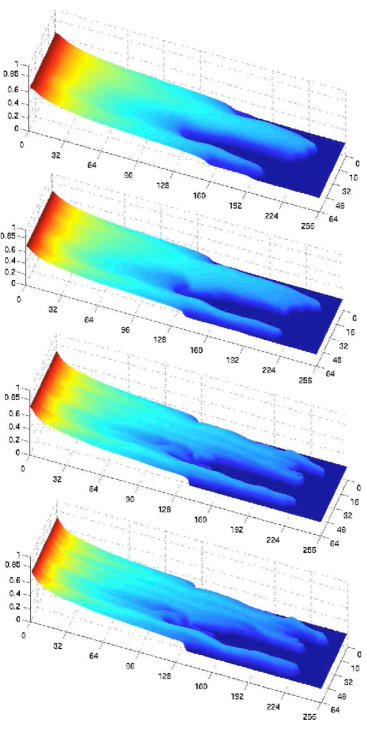
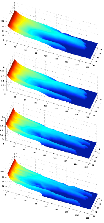
The boundary conditions, injection and production specifications for two-phase flow equations (1)-(2)) are as follows. For the horizontal slab geometry, injection is made uniformly along the left edge of the reservoir and the (total) production rate is taken to be uniform along the right edge; no flow is allowed along the edges appearing at the top and bottom of the reservoir in the graphics (Figures 6, 7, and 8).

In the case of a five-spot flood with diagonal grid (Figure 9), injection takes place at one corner and production at the diametrically opposite corner; no flow is allowed across the entirety of the boundary. In the case of a five-spot flood with the parallel grid, injection takes place at two corners (diametrically opposite), say left down and right up, and production in the diametrically ’off corners’, say right down and left up.

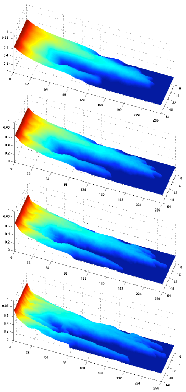
Figure 6. Water saturation surface plots for two-phase flow in a two-dimensional heterogeneous reservoir having $256$ m $\times$ $64$ m, with the coefficient of variation $C_{v}=0.5$ and viscous ratio 20. From top to bottom:$1)$ (KT dxd) scheme with $256\times 64$ grid; $2)$ (KT dxd) scheme with $512\times 128$ grid; $3)$ (KT two) scheme with $256\times 64$ grid.

Figure 7. Water saturation surface plots for two-phase flow in a two-dimensional heterogeneous reservoir having $256$ m $\times$ $64$ m, with the coefficient of variation $CV=1.2$ and viscous ratio 20. From top to bottom:$1)$ (KT dxd) scheme with $256\times 64$ grid; $2)$ (KT dxd) scheme with $512\times 128$ grid; $3)$ (KT two) scheme with $256\times 64$ grid.

Figure 8. Water saturation surface plots for two-phase flow in a two-dimensional heterogeneous reservoir having $256$ m $\times$ $64$ m, with the coefficient of variation $CV=2.2$ and viscous ratio 20. From top to bottom:$1)$ (KT dxd) scheme with $256\times 64$ grid; $2)$ (KT dxd) scheme with $512\times 128$ grid; $3)$ (KT two) scheme with $256\times 64$ grid.

(a) NT2D: $64\!\times\!64$ c lulas

(b) KTdxd: $64\!\times\!64$ c lulas

(c) NT2D: $128\!\!\times\!\!128$ c lulas

(d) KTdxd: $128\!\times\!128$ c lulas

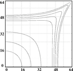
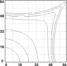
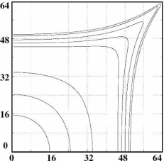
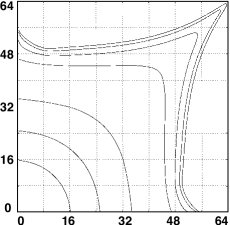
Figure 9. Water saturation level curves for two-phase flow in a five-spot well configuration. The SD2-2D scheme was used in pictures in the left column and the KTdxd was used in pictures in the right column.

3.1. Analyzing the Numerical Results. Conclusions

The Figures 6, 7 and 8 refer to a comparative study for the KT dimension by dimension and a genuinely two-dimensional KT schemes showing the water saturation surface plots after $350$ days of simulation for three different values for the strength of the heterogeneity of the fractal permeability field, $CV=0.5,1.2$ and $2.2$.

Note that the genuinely two-dimensional KT scheme gives a more accurate solution than the solutions computed by the KT dimension by dimension scheme for the same grid. In fact we observe that the KT dxd is only comparable in accuracy with one degree of refinement (see Figures 6, 7 and 8). The better accuracy of the genuinely two-dimensional approach is due to a more precise computation of the genuinely two-dimensional numerical fluxes, with respect to the one dimensional numerical fluxes in the dimension by dimension approach.

In the case of a five-spot geometry homogeneous reservoir, Figure 9 (diagonal grid) shows the saturation level curves after $260$ days of simulation obtained with KTdxd and SD2-2D schemes for two levels of spatial discretization. In this figure 9, the pictures on the left column are the results obtained with the SD2-2D scheme and the ones on the right were computed with the KTdxd scheme. In these Figures, the grid become finer from top to bottom, having $64\,\times\,64$ and $128\,\times\,128$ cells, respectively.

It is clear that the KTdxd scheme (right column pictures in Figures 9 is producing incorrect boundary behavior. Moreover as the computational grid is refined (right column and bottom picture in Figure 9) this problem seems to be emphasized indicating that the solution is not convergent.

The KTdxd scheme uses numerical fluxes in the $x$ and $y$ directions which can be viewed as generalizations of one-dimensional numerical fluxes. We state that this type of approximation for the fluxes leads to the incorrect boundary behavior discussed above. This incorrect boundary behavior led us to develop a new genuinely two-dimensional KT scheme. The results obtained with this new scheme can be seen in the left column of Figure 9. It is clear that we have corrected the boundary behavior just changing the approach from dimension by dimension to our two-dimensional approach. This fact indicates (but does not prove) our idea that computing two-dimensional numerical fluxes using straight generalizations of one-dimensional numerical fluxes may produce incorrect numerical solutions.

References

• Abreu et al. (2004a) E. Abreu, F. Furtado, D. Marchesin, and F. Pereira. Transitional waves in three-phase flows in heterogeneous formations. Computational Methods for Water Resources, I:609–620, 2004a.
• Abreu et al. (2004b) E. Abreu, F. Furtado, D. Marchesin, and F. Pereira. Three-phase flow in petroleum reservoirs. Proceedings of the Conference on Analysis, Modeling and Computation of PDEs and Multiphase Flow, in Celebration of James Glimm’s 70th Birthday, SUNY at Stony Brook. To appear, 2004b.
• Abreu et al. (2004c) E. Abreu, F. Furtado, and F. Pereira. On the numerical simulation of three-phase reservoir transport problems. Transport Theory Statist. Phys., 33(5-7):503–526, 2004c.
• Abreu et al. (2006) E. Abreu, F. Furtado, and F. Pereira. Three-phase immiscible displacement in heterogeneous petroleum reservoirs. Mathematics and computers in simulation, 73:2–20, 2006.
• Abreu et al. (2007) E. Abreu, Furtado F., F. Pereira, and S. Ribeiro. Central schemes for porous media flow. (Paper to be submited.), 1:6, 2007.
• Abreu et al. (2008) E. Abreu, Jim Douglas Jr., F. Furtado, and F. Pereira. Operator splitting for three-phase flow in heterogeneous porous media, 2008. To appear in: International Journal of Computational Science, 2008.
• Chavent and Jaffré (1986) G. Chavent and J. Jaffré. Mathematical Methods and Finite Elements for Reservoir Simulation, volume 17. Studies in Mathematics and its Applications, North-Holland, Amsterdam, studies in mathematics and its applications edition, 1986.
• Douglas et al. (1997) J. Douglas, Jr., F. Furtado, and F. Pereira. On the numerical simulation of waterflooding of heterogeneous petroleum reservoirs. Comput. Geosci., 1(2):155–190, 1997.
• Furtado and Pereira (2003) F. Furtado and F. Pereira. Crossover from nonlinearity controlled to heterogeneity controlled mixing in two-phase porous media flows. Comput. Geosci., 7(2):115–135, 2003.
• Glimm et al. (1993) J. Glimm, B. Lindquist, F. Pereira, and Q. Zhang. A theory of macrodispersion for the scale up problem. Transport in Porous Media, 13:97–122, 1993.
• Jiang and Tadmor (1998) G.-S. Jiang and E. Tadmor. Non-oscillatory central schemes for multidimensional hyperbolic conservation laws. SIAM Journal on Scientific Computing, 19:1892–1917, 1998.
• Kurganov and Petrova (2001) A. Kurganov and G. Petrova. A third-order semi-discrete genuinely multidimensional central scheme for hyperbolic conservation laws and related problems. Numer. Math., 88(4):683–729, 2001.
• Kurganov and Tadmor (2000) A. Kurganov and E. Tadmor. New high-resolution central schemes for nonlinear conservation laws and convection-diffusion equations. J. Comput. Phys., 160(1):241–282, 2000.
• Lax (1954) P.D. Lax. Weak solutions of non-linear hyperbolic equations and their numerical computation. Comm. Pure Appl. Math., 7:159–193, 1954.
• Nessyahu and Tadmor (1990) H. Nessyahu and E. Tadmor. Nonoscillatory central differencing for hyperbolic conservation laws. J. Comput. Phys., 87(2):408–463, 1990.
• Peaceman (1977) D. W. Peaceman. Fundamentals of Numerical Reservoir Simulation. Elsevier, New York, 1977.
• Raviart and Thomas (1977) P.-A. Raviart and J. M. Thomas. A mixed finite element method for 2nd order elliptic problems. In Mathematical aspects of finite element methods (Proc. Conf., Consiglio Naz. delle Ricerche (C.N.R.), Rome, 1975), pages 292–315. Lecture Notes in Math., Vol. 606. Springer, Berlin, 1977.
• Rusanov (1961) V. V. Rusanov. The calculation of the interaction of non-stationary shock waves with barriers. Ž. Vyčisl. Mat. i Mat. Fiz., 1:267–279, 1961.
• Van Leer (1979) B. Van Leer. Towards the ultimate conservative difference scheme. v. a second order sequel to godunov’s metthod. J. Comp. Phys., 32:101–136, 1979.