Inertial effects in Büttiker-Landauer Motor and Refrigerator at the Overdamped Limit
Abstract
We investigate the energetics of a Brownian motor driven by position dependent temperature, commonly known as the Büttiker-Landauer motor. Overdamped models () predict that the motor can attain Carnot efficiency. However, the overdamped limit (), contradicts the previous prediction due to the kinetic energy contribution to the heat transfer. Using molecular dynamics simulation and numerical solution of the inertial Langevin equation, we confirm that the motor can never achieve Carnot efficiency and verify that the heat flow via kinetic energy diverges as in the overdamped limit. The reciprocal process of the motor, namely the Büttiker-Landauer refrigerator is also examined. In this case, the overdamped approach succeeds in predicting the heat transfer only when there is no temperature gradient. Its found that the Onsager symmetry between the motor and refrigerator does not suffer from the singular behavior of the kinetic energy contribution.
pacs:
05.40.-a, 05.40.Jc, 05.10.Gg, 05.70.LnI Introduction
Since the industrial revolution, thermodynamics has been a guiding principle for the development of new technology. We are now entering the era of nanotechnology where we can construct and manipulate nanoscale objects as we desire. Realization of nanoscale machines is within our reach. However, we still have to overcome various issues. As the size of a system approaches to that of molecules, thermal fluctuations begin to play a significant role. It would be rather difficult to operate a nanomachine against strong thermal fluctuations. Instead, the nanomachine must be able to work harmoniously or even collaboratively with the fluctuations. In order to design such machines, we need to understand thermodynamics of small systems taking into account large thermal fluctuations. Furthermore, the molecular machinery in biological systems such as motor proteins are similarly subject to large thermal fluctuations. Thermodynamics, at the macromolecular level, is also essential in the investigation of such biological machines.
Unfortunately, since it was originally developed for macroscopic systems where fluctuations are negligible, standard thermodynamics is often powerless in cases where fluctuations dominate. We often resort to stochastic approaches such as Fokker-Planck equation or Langevin equation. Despite the fact that these approaches have been successfully used for many years, the relation between thermodynamics and stochastic methods is not well established. It was only 10 years ago when a general theory of energetics such as heat within the stochastic regime (stochastic energetics) sekimoto97 ; sekimoto98 ; sekimoto was developed. The validity of the theory needs to be systematically tested with experiment or first principles simulation.
When traditional thermodynamics was developed, Carnot engine played a key role as an idealized model. Similarly, Brownian motors reimann02 have been basic working models for systems dominated by thermal fluctuations. In particular, autonomous thermal engines such as the Feynman-Smoluchowski (FS) motor feynman and Büttiker-Landauer (BL) motor buttiker87 ; landauer88 , unlike other Brownian motors, do not require time-dependent external influence. These motors are driven solely by thermal fluctuations and their motility disappears when the motors become macroscopic in size.
There is no difficulty in the investigation of their motility using standard stochastic approaches. However, it was not straightforward to investigate the thermodynamics of these systems. In his celebrated textbook feynman , Feynman attempted to investigate the thermodynamics of the FS motor and concluded that it can reach Carnot efficiency. Yet, he overlooked the effect of fluctuations and later it was shown that the heat transfer between two heat reservoirs never ceases even when the motor moves quasistatically and thus it is not possible to reach the Carnot efficiency sekimoto97 ; parrondo96 ; hondou98 . Even when the average velocity of the motor is zero, fluctuations around the mean value can transport some energy. It is this fluctuation that transports heat. Recently, a simpler model of the FS motor was developed and their result confirms the presence of such heat transfer vandenbroeck04 . Similar heat transfer was investigated in the problems of adiabatic piston kestemont00 and shared piston vandenbroeck01 . The reverse process of the FS motor, namely the FS refrigerator has also been studied using various models jarzynski99 ; vandenbroeck06 ; nakagawa06 .
The BL motor is just an overdamped Brownian particle in a periodic potential field subject to spatially inhomogeneous temperature. When temperature changes across a potential barrier, the Brownian particle jumps over the barrier more often from the hot side to the cold side than the other way buttiker87 ; landauer88 ; bier96 . Therefore, Brownian particles move in one direction on average. Whereas the FS motor is simultaneously in contact with two heat baths, the BL motor moves from one heat bath to another by itself. Therefore, the BL motor is a different class of Brownian motor from the FS motor. In order for the BL motor to operate continuously, it must be thermalized with the local environment before entering the next heat bath. Thus, it works better in the overdamped limit but fails in the underdamped limit blanter98 .
Like the FS motor, there is no difficulty in explaining the motility of the BL motor. However, the thermodynamics of this system is not straightforward. Intuitively we expect non-vanishing heat transfer even when the average current is zero since the Brownian particles can move back and forth between the hot and cold regions by thermal fluctuations derenyi99 ; hondou00 . Despite this anticipation, some previous investigation claimed that the BL motor can reach the Carnot efficiency matsuo00 ; asfaw04+05+07 and under certain conditions can act as a refrigerator, attaining the corresponding Carnot coefficient of performance asfaw04+05+07 . It turns out, however, that the overdamped Langevin approach fails to predict such heat transfer for the BL motor while it worked fine for the FS motor sekimoto97 ; hondou98 . It appeared that even when the system is in the overdamped regime, inertial mass () apparently plays a critical role in certain thermodynamic processes. In fact, heat evaluated by assuming at the beginning does not agree with the result obtained by taking the limit at the end. This singularity has been phenomenologically predicted derenyi99 ; hondou00 but not yet experimentally tested. Due to the lack of experimental confirmation, this issue is still a subject of debate asfaw04+05+07 ; ai05+06 .
In this paper, we investigate the BL motor and its reciprocal process, the BL refrigerator, using stochastic energetics based on Langevin approach, with and without inertial effects and compare the results with molecular dynamics simulation. Our main objective is to check the failure of the overdamped Langevin method and the validity of the inertial Langevin method by comparing the results with molecular dynamics simulation. The overdamped method appears to fail for the BL motor involving inhomogeneous temperature but works fine for the BL refrigerator operated with homogenous temperature. On the other hand, these two processes are related to one another through Onsager’s symmetry, which is not obvious for a system with inhomogeneous temperature, prompting us to investigate the validity of the Onsager symmetry in the overdamped regime vankampen91 . We will check the validity numerically, taking into account inertial effects.
In the next section, we introduce a concrete model of BL motor/refrigerator which can be investigated by both Langevin and molecular dynamics simulations. In section III, a brief heuristic discussion based on the overdamped Langevin equation is given. In section IV the results of the overdamped approach are compared with numerical simulations of the Langevin equation taking inertia into account and the molecular dynamics simulation. Further discussion and conclusion follow in the final section.
II The model and methods
II.1 The model
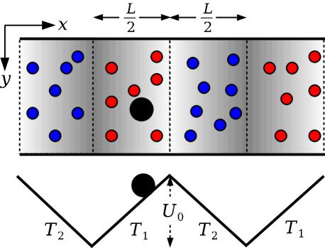
We consider a chain of two-dimensional cells aligned in the direction as illustrated in Fig. 1. Each cell has a width of and is filled with gas particles confined in the cell they belong to. No direct heat exchange between cells through the walls is permitted. The gas particles in a cell act as a heat reservoir with its own temperature, independent of the temperature in other cells. Brownian particles of mass are placed in the cells. Unlike the gas particles, the Brownian particles are allowed to move freely from one cell to another through the walls and they are also subject to a potential field , which is periodic in the direction with a periodicity and constant in the direction. For simplicity, we use a piecewise-linear potential:
| (1) |
where is the potential height. The coordinate is chosen such that the location of potential maxima/minima coincide with the cell boundaries as shown in Fig. 1. In addition to the periodic potential, a constant external force is exerted on the Brownian particles. We further assume that temperature is periodic with the same periodicity as the potential and piecewise constant:
| (2) |
Temperature is measured in energy unit ().
For technical simplicity, we consider only two cells (cell 1 for and cell 2 for ) with a periodic boundary condition instead of infinitely long chains.
II.2 Langevin approaches
Molecular Dynamics (MD) simulation is a useful tool to investigate this kind of model. However, a simpler mathematical model is desirable since MD simulation is computationally quite demanding. Apart from long-time fluid dynamical effects in two dimensions, the motion of the Brownian particle in the direction can be investigated by the one-dimensional Langevin equation:
| (3) |
where and are position and velocity of the Brownian particle and is a standard Gaussian white noise:
| (4) |
Here, and later on, an overdot refers to derivative taken with respect to time and a prime means derivative taken with respect to space. The position-dependent friction coefficient is assumed to be periodic and piece-wise constant in the same way as temperature:
| (5) |
It has been shown that the Langevin Eq. (3) correctly predicts the behavior of Brownian particles. However, due to its mathematical difficulty, further approximation is often used. When the relaxation time is much smaller than a mechanical time scale , the inertial term in Langevin equation (3) is usually neglected. Setting in Eq. (3) we obtain a popular overdamped Langevin equation,
| (6) |
While this equation is widely used in many different subject areas, we must be careful with since both and are zero at the same time. Strictly speaking, the overdamped condition should be satisfied only in the sense of the limit .
Further complication arises when temperature or friction coefficient depends on the position. Simple omission of the inertial term does not lead to the correct overdamped Langevin equation. One can also study stochastic processes in the overdamped limit by the equivalent Fokker-Planck equation. There is, however, no universal Fokker-Planck equation that describes a system with non-uniform temperature. Van Kampen vankampen88 found that a particular form of Fokker-Planck equation depends on the details of each system. For our model (overdamped Brownian particle subject to inhomogeneous temperature) the appropriate Fokker-Plank equation is given by,
| (7) |
While solving Eq. (7) for the piecewise constant temperature (2), the proper boundary conditions are and , where is infinitesimally small boundary .
Corresponding to the Fokker-Planck equation (7), the correct form of the overdamped Langevin equation, in the Stratonovich interpretation, is
| (8) |
as derived in sancho92 ; jayannavar95 . In this paper, we shall call Eq. (8) the overdamped Langevin equation and refer to Eq. (3) as the inertial Langevin equation.
As an indicator of overdamping, we introduce a dimensionless frictional coefficient:
| (9) |
When , the system is in the overdamped regime.
II.3 Stochastic energetics
We investigate the thermodynamic behavior of the BL system using stochastic energetics introduced by Sekimoto sekimoto97 ; sekimoto98 ; sekimoto . Heat flux from the gas particles in the -th cell to the Brownian particles is defined as
| (10) |
where indicates ensemble average taken while the Brownian particles are located in the -th cell. Using the inertial Langevin equation (3), Eq. (10) can be evaluated in three terms:
| (11) |
where the first two terms on the rhs are the kinetic energy and potential energy contribution to the heat flux, respectively, and the last term is the Joule heat.
Work done on a Brownian particle by the external force in each cell is given by,
| (12) |
In the steady state, the net energy flux to the Brownian particles must be zero, and thus the energy gained by the Brownian particles in cell 1 must be cancelled by the energy loss in cell 2. Therefore, heat flux from cell 1 to cell 2 via the Brownian particles is defined as
| (13) |
II.4 Molecular Dynamics simulation
In order to check the validity of the Langevin approach, we performed intensive molecular dynamics simulation. In our MD simulation the heat bath consists of two-dimensional hard disks of mass and diameter . The Brownian particle is of mass and diameter . Inclusion of external forces significantly reduces the numerical advantage of hard disk MD simulation. However our algorithm (see Appendix A) is fast enough to realize a sufficient number of trajectories for ensemble average.
In order to compare the results of Langevin approaches with that of MD simulation, we need to find the corresponding frictional coefficient. We use an analytical expression obtained for an ideal gas meurs04 :
| (14) |
where is the density of the gas. Note that this ideal does not depend on . Alternately, we could use measured in MD simulation. Infact, we can get a better agreement between MD simulation and Langevin approaches if the measured values are used. However, the measured values depend on , hindering the real mass dependency of the Langevin equation. Therfore, we use the theoretical frictional coefficient (14) in the Langevin equations (3) and (8).
In all our MD simulations we use gas particles (, ) in each cell, with the size of each cell being so that the density . The spatial period of the piece-wise linear potential is and the barrier height . As the temperature of the reservoirs change during the course of the simulation there is no well defined stationary state. However, all our simulations were carried out using a sufficiently large number of gas particles so that the system remains in a quasi-steady state for a sufficiently long period of time, enabling us to measure the various physical quantities properly.
III Heuristic discussion with the overdamped model
In this section we first review the known properties of the BL motor and its reciprocal process BL refrigerator, in the overdamped limit. When the temperature of the cells are different (), the Brownian particles in the high temperature cell can reach a higher potential energy region than those in the low temperature cell. Hence, the Brownian particles tend to move from the hot cell to the cold cell over the potential barrier. At the other cell boundary the potential is minimum and both cold and hot Brownian particles can easily cross to the other side. Therfore, the Brownian particles flow in the positive direction on average even in the absence of external force (). When an external load is applied (), the Brownian particles can do work against it as a motor.
Asymmetry in the spatial distribution of the Brownian particles due to the temperature difference is the main driving of this motor. The overdamped Langevin equation (8) or Fokker-Planck equation (7) provide an analytical expression of the spatial distribution, from which we obtain the average velocity of the motor (See Appendix B)
| (15) |
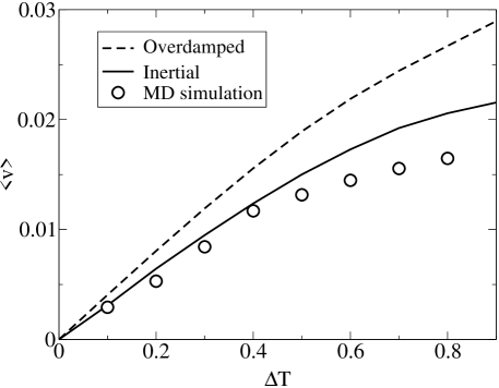
where and . In the absence of external force (), Equation (15) is always positive for and hence the Brownian particles move in the positive direction as expected. In fact, particle distribution and velocity in the overdamped regime agree reasonably well with the results obtained from numerical simulation of the inertial Langevin equation and molecular dynamics simulation (see Figs. 2 and 3), suggesting the validity of the overdamped Langevin equation.
Now, we consider the thermodynamic efficiency of the BL motor. Based on the successful prediction of particle distribution and velocity it is natural to use the overdamped Langevin approach for other quantities such as efficiency. Applying the overdamped Langevin equation (8) to the definition of heat (10), the heat flux from the heat bath to the Brownian particles in cell is given by
| (16) |
Comparing this equation with Eq. (11), the first term in the rhs of Eq. (16) corresponds to the kinetic energy contribution . However, due to periodic boundary condition and Eq. (14), this kinetic energy contribution vanishes matsuo00 and we obtain . Hence, we find the efficiency of the motor
| (17) |
where . When the motor is in a stalled state, (), we can show that the efficiency reaches the Carnot efficiency .
This result is puzzling since at the moment a Brownian particle enters the cold bath it is carrying of kinetic energy. When it is thermalized with the cold bath, of heat dissipates into the cold bath. This heat dissipation takes place whenever the Brownian particle crosses a temperature boundary and it is irreversible. Due to diffusion the crossing occurs even when the average velocity vanishes, and this irreversible heat due to thermal fluctuation of Brownian particles never ceases as long as there is a steep temperature gradient. Derényi-Astumian derenyi99 and Hondou-Sekimoto hondou00 have pointed out that the kinetic energy contribution is the dominant channel of heat transfer between two cells and thus the efficiency of the BL motor cannot reach the Carnot efficiency. This situation is similar to the case of the FS motor parrondo96 ; sekimoto97 .
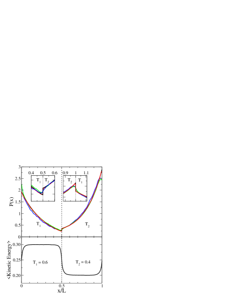
An interesting question is why the overdamped Langevin approach failed for the BL motor whereas it worked fine for the FS motor. Derényi-Astumian derenyi99 and also Hondou-Sekimoto hondou00 phenomenologically answered this question. Consider the thermal velocity . When a Brownian particle crosses the temperature boundary, it will not be immediately thermalized and there is a narrow region where the average kinetic energy of the Brownian particle does not coincide with the temperature of the reservoir (see lower panel of Fig. 3). In the overdamped limit () this region vanishes, justifying the use of the overdamped approach. However, the effective temperature gradient is . Hence, the heat current is proportional to and diverges as . This singularity implies that the overdamped regime that assumes is not equivalent to the overdamped limit . Apparently, the FS motor does not have this problem sekimoto97 . One of our objectives is to verify this singular behavior by numerical simulations.
Next, we turn to the BL refrigerator. We assume and apply a weak external force to the Brownian particle. Due to the external force, the Brownian particle drifts in the direction of and its average velocity in the overdamped limit can be obtained from Eq. (15). Unlike the motor case, the temperature is uniform throughout the system and thus the kinetic energy does not contribute significantly to the heat exchange between the cells. Again using the overdamped model, the heat flux absorbed by the Brownian particle from the -th reservoir is obtained from Eq. (16) as
| (18) |
where the first term is the potential energy contribution and the second term the Joule heat . Since and we can have positive for sufficiently small , indicating that cell 1 is refrigerated. Since there is no singular behavior due to temperature change, the overdamped model may be good enough. However, as soon as refrigeration induces a temperature difference between the cells, the heat transfer due to the kinetic energy reduces the power of refrigeration. Our second objective is to investigate whether the overdamped model is sufficient and if the refrigeration can be sustained against the heat leak due to the kinetic energy.
The BL motor and refrigerator are a result of cross effect between the external force and the temperature difference . Assuming they are small, we can make a connection between the motor and refrigerator using linear irreversible thermodynamics expressed by
| (19) |
where the transport coefficients are defined as
| (20) |
Here, the partial derivatives are evaluated at and . In the overdamped case we can obtain all Onsager coefficients from Eqs. (13), (15), and (16), as
| (21) |
where . These coefficients support the Onsager symmetry . Moreover, Eq. (21) indicates , implying no entropy production degroot and thus the motor operates at the Carnot efficiency. Hence the overdamped model again erroneously predicts the highest possible efficiency. The singular behavior of at casts some doubt on the Onsager symmetry since the two limits and do not commute. Our third objective is to numerically investigate the validity of linear irreversible theory and the Onsager symmetry at the overdamped limit.
IV Results
IV.1 Motor
First we show in Fig. 3 that the numerical solution of overdamped Langevin equation (8) agrees perfectly with the solution of the corresponding Fokker-Planck equation (7), confirming that the extra term in Eq. (8) is necessary. Furthermore, the results of overdamped Langevin equation are in good agreement with the numerical results from inertial Langevin equation (3) and molecular dynamics simulation, except for narrow regions at the temperature boundaries (see the insets in Fig. 3). Although it is in general small, this error in the overdamped regime should not be overlooked.
As we discussed in section III, the overdamped Langevin method assumes that the Brownian particles are locally in equilibrium with the the thermal reservoir. Therefore, the average kinetic energy of the Brownian particles is assumed to be the same as the local temperature of the heat bath. This assumption, however, fails near the temperature boundaries since the Brownian particles entering from one temperature region to another are not immediately thermalized with the new environment even when the mass is very small as Fig. 3 indicates. The size of the transition region is the thermalization length . In the overdamped limit (), indeed the transition region vanishes but only slowly as .
It turns out that such a subtle error in the overdamped Langevin method does not lead to large errors in certain quantities obtained from it. Figure 2 shows that the overdamped Langevin equation predicts the average velocity as well as the inertial Langevin equation does. Due to this success we feel safe to use the overdamped approach to compute other quantities. However, the calculation of the heat is a different story. As we discussed in the previous section, the overdamped approach predicts that the heat transfer between the cells is only from potential energy contribution. However, Hondou-Sekimoto hondou00 pointed out that the narrow transition region plays a dominant role in heat transfer and the overdamped Langevin equation fails in the investigation of heat calculation. The inertial Langevin approach concludes that the kinetic energy contribution is actually dominant.
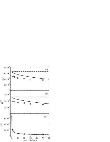
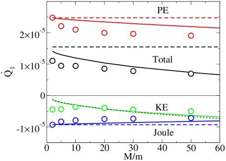
Using scaling arguments, Derényi-Astumian derenyi99 and Hondou-Sekimoto hondou00 predicted that the kinetic energy contribution diverges as at . Figure 4 clearly shows such a singularity in good agreement with their theory and confirms . We also find from Fig. 4 that result obtained from the inertial Langevin equation approaches the MD simulation result as the mass ratio increases. Even for small , the inertial Langevin equation predicts the correct order of magnitude of the motor velocity and the heat flows, though, in general, the Langevin approach is not applicable in such a case. The motor velocity and heat flow via potential energy predicted by the overdamped model, deviate from the inertial Langevin equation and MD simulation result as the mass ratio increases because the inertial effect becomes too large to be ignored. The good agreement between the inertial Langevin equation and the molecular dynamics simulation, shows that Sekimoto’s definition of stochastic energetics predicts the heat correctly even when temperature is spatially inhomogeneous.
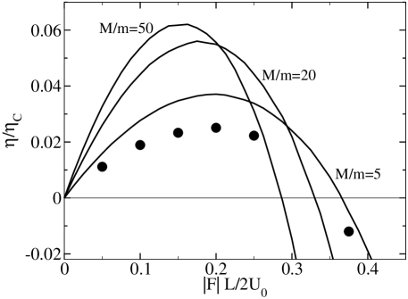
In Fig. 5, we plot the efficiency of the motor normalized by Carnot efficiency , as a function of the external load normalized by the magnitude of the force exerted by the periodic potential energy. In contradiction to the overdamped model, the efficiency is far below the Carnot limit. While this result was phenomenologically argued for in derenyi99 ; hondou00 , here we confirmed with molecular dynamics simulation and numerical solution of inertial Langevin equation that the kinetic energy contribution greatly reduces the efficiency. Even when the motor is operated at the quasistatic limit with a stall force, the irreversible heat transfer via kinetic energy persists and thus the Carnot limit is unattainable. Furthermore, the divergence of at diminishes the efficiency of the motor to zero, in the overdamped limit.
IV.2 Refrigerator
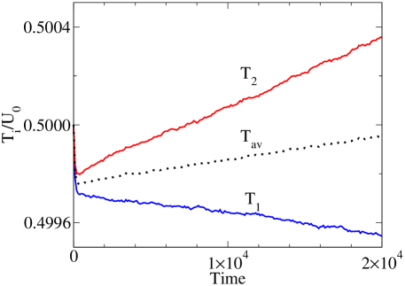
In the refrigerator mode, two cells initially have the same temperature and the Brownian particles are driven by an external force . In Fig. 6, MD simulation illustrates the cooling of cell 1 at the expense of the heating of cell 2. Note however, that the average temperature increases with time as Joule heat is dissipated in both the cells. In the Langevin approach, we cannot see such temperature changes since the temperature needs to be kept constant. However, it allows us to investigate heat transfer between the cells. Figure 7 shows the components of heat from cell 1 to the Brownian particles as a function of . The potential energy contribution increases linearly with whereas Joule heat decreases () as [see Eq. (18)]. For sufficiently small , the potential energy contribution wins and hence the Brownian particles extract heat from cell 1 and dump it in cell 2. There is an optimal at which the cooling effect is maximum. The agreement between the overdamped and inertial Langevin equations and with the molecular dynamics simulation is good for and .
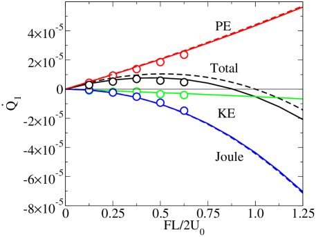
Since temperature is uniform, we don’t expect significant kinetic energy contribution. However in Fig. 7, we found that there is a small amount of kinetic energy contribution which is absent in the overdamped approach. In the overdamped regime we assume that the change in potential energy immediately dissipates into the reservoir. However, with a finite mass, the potential energy is first converted to kinetic energy which dissipates at a later time. For example, when a Brownian particle slides down the potential slope near a cell boundary, the potential energy change is transported to the next cell as kinetic energy where it is dissipated as heat. The amount of “unthermalized” kinetic energy the Brownian particles acquire from the potential energy is approximately,
| (22) |
which is linear with through in agreement with the result of the inertial Langevin equation (see Fig. 7). Both this kinetic energy contribution and the potential energy contribution are in proportion to , yet the magnitude of is negligibly smaller than that of at the overdamped limit. Therefore, the refrigeration is still possible. Figure 8 shows that the PE contribution approaches the overdamped model as . The KE contribution approaches to zero as , in good agreement with the phenomenological prediction (22). Figures 7 and 8 both show that the overdamped model is in good agreement with the inertial Langevin equation as well as MD simulation in predicting the velocity and heat flows.
The overdamped Langevin equation seems to work well for the refrigerator. However, the cooling effect creates a temperature difference between the two reservoirs and the overdamped approach again fails. In turn, the temperature difference induces a thermodynamic force opposing the external force , through the Brownian motor mechanism. As the temperature difference increases, the motor and refrigerator effects eventually cancel each other, so that the average velocity of the Brownian particle becomes zero and the cooling ceases.
IV.3 Onsager symmetry
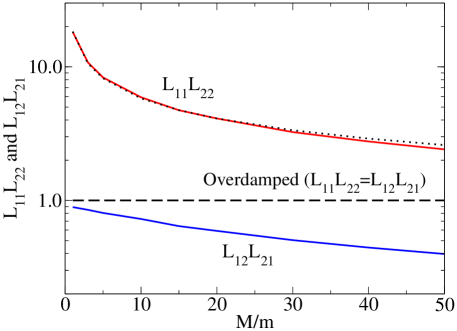
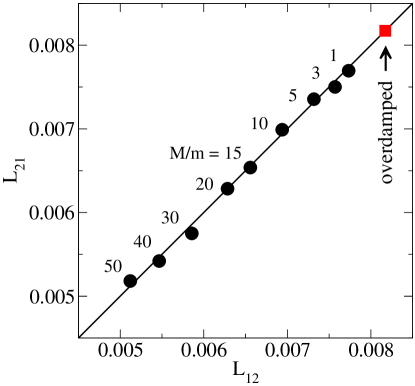
As discussed in section III, we need to evaluate the transport coefficients (20) with a certain care. Since the heat transfer diverges when the limit is taken before , we first evaluate the coefficients at the finite mass numerically from the response curves like Figs. 2 and 7. Then, we reduce the mass toward . Figure 9 shows that as decreases, the product of off-diagonal coefficients approaches to the result of overdamped Langevin equation obtained from Eq. (21). However, the product of diagonal coefficients diverges as , reflecting the divergence of . As expected, the off-diagonal coefficients do not suffer from the singular inertial effect. Furthermore, Fig. 9 shows that for all values of , indicating large entropy production consistent with the very low efficiency. Finally, Fig. 10 numerically verifies the Onsager symmetry for all masses within the accuracy of simulation and that the overdamped model (21) predicts the correct overdamped limit.
V Discussion
In this paper, we investigated the thermodynamic properties of the BL motor and refrigerator using Langevin equations and molecular dynamics simulation. For mechanical properties such as the velocity of the Brownian particles, we observed reasonable agreement between overdamped Langevin equation and molecular dynamics simulation. However, the overdamped Langevin equation failed to predict thermodynamic properties such as the heat transfer. On the other hand, we found good agreement between the inertial Langevin equation and molecular dynamics simulation even in the overdamped regime. Therefore, we conclude that the inertial mass plays a significant role even in the overdamped limit. The main effect of the inertial mass is the kinetic energy contribution to the heat transfer. We confirmed that the kinetic energy contribution is dominant when two cells have different temperature and verified a previous phenomenological prediction, that the irreversible kinetic energy contribution diverges as at the overdamped limit.
Recently, Van den Broeck vandenbroeck07 investigated the efficiency of Brownian motors using linear irreversible thermodynamics and concluded that, in principle, Carnot efficiency can be attained. He argues that when the load is small, the temperature difference drives the motor in the forward direction and at the same time the motor transfers heat from the high temperature reservoir to the low temperature reservoir. As the load exceeds the stall force, the motor moves backward, transferring heat against the temperature gradient as a heat pump. In an ideal system, the direction of velocity and heat are reversed at the same magnitude of the external force. Hence, the thermodynamic fluxes and simultaneously vanish despite and not being zero. This can only happen when and thus Carnot efficiency is achieved.
In our case, the direction of coincides with the direction of , and both and vanish at the stall force. However, flows from the hot to cold reservoir regardless of the direction of . Therefore, not necessarily vanishes. In fact, it never vanishes and the Carnot efficiency cannot be achieved in the BL system. The efficiency of the BL motor is significantly reduced by the kinetic energy contribution and vanishes at the overdamped limit.
Dérenyi-Astumian derenyi99 have argued that if we could prevent the re-crossing of the Brownian particle over the temperature boundary, such irreversible heat transfer could be arbitrarily reduced and thus the efficiency would be greately improved. They proposed to place a gate at each temperature boundary which prevents Brownian particles from crossing the boundary back and forth multiple times during a short period of time. If such a gate is possible, the motor could reach Carnot efficiency. However, it is not clear at present how to construct such a gate without reducing the particle velocity. Based on a naive consideration one might expect significant reduction of the kinetic energy contribution by optimizing the potential profile and the location of the temperature boundary. Unfortunately, the reduction of heat transfer always results in the reduction of the motor velocity as well and the gain in the efficiency is very limited benjamin .
Recently, Humphrey et al. humphrey02 proposed a quantum Brownian heat engine which achieves Carnot efficiency. In this model, reversible particle exchange between two cells is achieved by filtering the energy of the particle, without violating second law. The filter only allows particles having a certain energy, for which the Fermi-Dirac distribution in the two cells coincide, to pass through. This ensures that the particle flow does not alter the thermal distribution in either cell so that there is no kinetic energy contribution. Hence, the heat engine attains Carnot efficiency in the quasistatic limit. Whether a similar heat engine can be devised in the classical regime is not clear.
VI Acknowledgments
We would like to thank Ken Sekimoto and C. Van den Broeck for useful discussion. The computer simulation was partly carried out at the Alabama Supercomputer Center.
Appendix A Hard Disk Molecular Dynamics Simulation
Our hard disk molecular dynamics simulation is based on a usual event-driven algorithm rapaport . In the case of collision between two gas particles the collision time can be obtained analytically as given in rapaport . However, since the Brownian particle is subject to forces due to the piece-wise linear potential and the external load , the calculation of collision time between a Brownian particle and a gas particle is not straightforward. Suppose that we know the relative position r and relative velocity v of a Brownian particle with respect to a gas particle at time . We want to find the time , at which they collide. The distance between two particles at the moment of impact is and hence
| (23) |
where a is a constant acceleration of the Brownian particle. (Note that the gas particle has no acceleration.) To find , we rewrite Eq. (23) as a quartic equation for
| (24) |
where , , , and . Using a standard method hacke41 , we find four solutions
| (25) |
where,
| (26) | |||||
| (27) | |||||
| (28) |
and is a real solution of an auxiliary equation,
| (29) |
The analytical solutions to the cubic equation (29) are given in press .
The correct collision time corresponds to the smallest positive real root of Eq. (25), if it exists. Despite having analytical solutions this algorithm occasionally fails, particularly when the acceleration is significantly small because some of the coefficients become extremely large causing bit-off errors. To overcome this difficulty, we improve the accuracy of the roots by iterating the Newton-Raphson press steps a few times starting from the analytical solution to Eq. (29). We found that the present algorithm is faster than directly solving the quartic equation (24) by the Newton-Raphson method.
Appendix B Analytical Expressions in Overdamped Case
We derive analytical expressions for steady state density and current . The Fokker-Planck equation for steady states is simply , where the particle current is defined by
| (30) |
In our model, the Fokker-Planck equation for the -th cell is given by
| (31) |
where the net force is defined as . We consider only weak external forces so that it does not destroy the potential barrier and hence we assume . Then, we find general solutions:
| (32) | ||||
| (33) |
where and are the constants of integration. The corresponding currents are . Since temperature and frictional coefficient are discontinuous at the cell boundaries, the density does not have to be continuous. However, the current must be continuous (). From Eq. (30), we find the magnitude of the density discontinuity as and boundary . These boundary conditions along with normalization of the density are sufficient to determine the integral constants. After obtaining an expression for and the integral constants, we obtain a general expression for the average velocity [Eq. (15)] from a general relation . The particle density in each cell is obtained from Eqs. (32) and (33).
References
- (1) K. Sekimoto, J. Phys. Soc. Jpn. 66, 1234 (1997).
- (2) K. Sekimoto, Prog. Theor. Phys. Suppl. 130, 17 (1998).
- (3) K. Sekimoto, Stochastic Energetics (Springer, in preparation).
- (4) P. Reimann, Phys. Rep. 361, 57 (2002).
- (5) R. P. Feynman, R. B. Leighton, and M. Sands, The Feynman Lectures on Physics (Addison Wesley, Reading, MA, 1966), Vol. I, Chap. 46.
- (6) M. Büttiker, Z. Phys. B 68, 161 (1987).
- (7) R. Landauer, J. Stat. Phys. 53, 233 (1988).
- (8) J. M. R. Parrondo and P. Español, Am. J. Phys. 64, 1125 (1996).
- (9) T. Hondou and F. Takagi, J. Phys. Soc. Jpn. 67, 2974 (1998).
- (10) C. Van den Broeck, R. Kawai, and P. Meurs, Phys. Rev. Lett. 93, 090601 (2004).
- (11) E. Kestemont, C. Van den Broeck, and M. Malek Mansour, Europhys. Lett. 49, 143 (2000).
- (12) C. Van den Broeck, E. Kestemont, and M. Malek Mansour, Europhys. Lett. 56, 771 (2001).
- (13) C. Jarzynski and O. Mazonka, Phys. Rev. E 59, 6448 (1999).
- (14) C. Van den Broeck and R. Kawai, Phys. Rev. Lett. 96, 210601 (2006)
- (15) N. Nakagawa and T. S. Komatsu, Europhys. Lett. 75, 22 (2006)
- (16) M. Bier and R. D. Astumian, Bioelectrochem. Bioenerg. 39, 67 (1996).
- (17) Y. M. Blanter and M. Büttiker, Phys. Rev. Lett. 81, 4040 (1998).
- (18) I. Derényi and R. D. Astumian, Phys. Rev. E 59, R6219 (1999).
- (19) T. Hondou and K. Sekimoto, Phys. Rev. E 62, 6021 (2000).
- (20) M. Matsuo and S. -I. Sasa, Physica A 276, 188 (2000)
- (21) M. Asfaw and M. Bekele, Eur. Phys. J. B 38, 457 (2004); Phys. Rev. E 72, 056109 (2005); Physica A 384, 346 (2007).
- (22) B. -Q. Ai, H. -Z. Xie, D. -H. Wen, X. -M. Liu, and L. -G. Liu, Eur. Phys. J. B 48, 101 (2005); B. -Q. Ai, L. Wang, and L. -G. Liu, Phys. Lett. A 352, 286 (2006).
- (23) N. G. van Kampen, J. Stat. Phys. 63, 1019 (1991).
- (24) N. G. van Kampen, IBM J. Res. Dev. 32, 107 (1988).
- (25) The boundary conditions for a system with inhomogeneous temperature is discussed in Ref. landauer88 . Different boundary conditions, namely and are often used in the literature bier96 ; asfaw04+05+07 . However, these boundary conditions are not consistent with the physical system under consideration. Indeed, the solution obtained with these boundary conditions disagrees with the results of our molecular dynamics simulation both qualitatively and quantatively.
- (26) J. M. Sancho, M. S. Miguel, and D. Duerr, J. Stat. Phys. 28, 291 (1982).
- (27) A. M. Jayannavar and M. C. Mahato, Pramana J. Phys. 45, 369 (1995).
- (28) P. Meurs, C. Van den Broeck, and A. Garcia, Phys. Rev. E 70, 051109 (2004).
- (29) S. R. de Groot and P. Mazur, Non-Equilibrium Thermodynamics (Dover, New York, 1984).
- (30) C. Van den Broeck, Adv. Chem. Phys. 135, 189 (2007).
- (31) R. Benjamin and R. Kawai (in preparation).
- (32) T. E. Humphrey, R. Newbury, R. P. Taylor, and H. Linke, Phys. Rev. Lett. 89, 116801 (2002).
- (33) D. C. Rapaport, The Art of Molecular Dynamics Simulation (Cambridge University Press, Cambridge, UK, 2004).
- (34) J. E. Hacke, Jr., Am. Math. Monthly 48, 327 (1941); See also Handbook of Mathematical Functions With Formulas, Graphs, and Mathematical Tables, ed. M. Abramowitz and I. A. Stegun, (US. National Bureau of Standards, 1972).
- (35) W. H. Press, B. P. Flannery, S. A. Teukolsky, and W. T. Vetterling, Numerical Recipes in FORTRAN, 2nd ed. (Cambridge University Press, Cambridge, England, 1992).