UCLA/08/TEP/10
MIT-CTP-3937
NSF-KITP-08-48
Saclay-IPhT–T08/054
SLAC–PUB–13161
An Automated Implementation of On-Shell Methods for One-Loop Amplitudes
Abstract
We present the first results from BlackHat, an automated C++ program for calculating one-loop amplitudes. The program implements the unitarity method and on-shell recursion to construct amplitudes. As input to the calculation, it uses compact analytic formulæ for tree amplitudes for four-dimensional helicity states. The program performs all related computations numerically. We make use of recently developed on-shell methods for evaluating coefficients of loop integrals, introducing a discrete Fourier projection as a means of improving efficiency and numerical stability. We illustrate the numerical stability of our approach by computing and analyzing six-, seven- and eight-gluon amplitudes in QCD and comparing against previously-obtained analytic results.
pacs:
11.15.Bt, 11.55.Bq, 12.38.BxI Introduction
The Large Hadron Collider (LHC) will soon begin exploration of the electroweak symmetry breaking scale. It is widely anticipated that physics beyond the Standard Model will emerge at this scale, leading to a breakthrough in our understanding of TeV-scale physics. A key ingredient in this quest is the precise understanding of the expected Standard Model backgrounds to new physics from both electroweak and QCD processes. In the absence of such an understanding, new physics signals may remain hidden, or backgrounds may be falsely identified as exciting new physics signals.
Quantitatively reliable QCD predictions require next-to-leading order (NLO) calculations NLMLesHouches . For a few benchmark processes, such as the rapidity distribution of electroweak vector bosons NNLOVrap , the transverse-momentum distribution of the boson at moderate , and the total cross sections for production of top quark pairs and of Higgs bosons HNNLO , the higher precision of next-to-next-to-leading order (NNLO) results may be required NLMLesHouches . For most other processes, NLO precision should suffice. However, there are many relevant processes that need to be computed, particularly those with high final-state multiplicity. Such processes are backgrounds to the production of new particles that have multi-body decays. To date, no complete NLO QCD calculation involving four or more final-state objects (particles or jets) is available. (In electroweak theory, however, fermions has been evaluated ElectroWeak4f using the integral reduction scheme of Denner and Dittmaier Denner .) NLO corrections require as ingredients both real-radiative corrections and virtual corrections to basic amplitudes. The structure of the real-radiative corrections — isolation of infrared singularities and their systematic cancellation against virtual-correction singularities — is well understood, and there are general methods for organizing them GG ; GGK ; CS . Indeed, the most popular of these methods, the Catani-Seymour dipole subtraction method CS , has now been implemented in an automatic fashion GK . The infrared divergences of virtual corrections, needed to cancel the divergences from integrating real radiation over phase space, are also understood in general GG ; KST . The main bottleneck to NLO computations of processes with four or more final-state objects has been the evaluation of the remaining ingredients, the infrared-finite parts of the one-loop virtual corrections.
As the number of external particles increases, the computational difficulty of loop-amplitude calculations using traditional Feynman diagrams grows rapidly. Technologies that have proven useful at tree level, such as the spinor-helicity formalism SpinorHelicity , do not suffice to tame these difficulties. In the past few years, several classes of new methods have been proposed to cope with this rapid growth OtherApproaches ; AguilaPittau ; Binoth ; Denner ; EGZ ; XYZ , including on-shell methods UnitarityMethod ; Zqqgg ; DDimUnitarity ; TwoLoopAllPlus ; BCFUnitarity ; OtherUnitarity ; BCFRecursion ; BCFW ; DoublePole ; Bootstrap ; Genhel ; OtherBootstrap ; BCFCutConstructible ; BMST ; OPP ; BFMassive ; OnShellReview ; Forde ; EGK ; CutTools ; GKM ; OPP2 ; MOPP which are based on the analytic properties of unitarity and factorization that any amplitude must satisfy OldUnitarity ; GeneralizedUnitarityOld . These methods are efficient, and display very mild growth in required computer time with increasing number of external particles, compared to a traditional Feynman-diagrammatic approach. The improved efficiency emerges from effectively reducing loop calculations to tree-like calculations. Efficient algorithms can then be employed for the tree-amplitude ingredients.
One of the principal on-shell technologies is the unitarity method, originally developed in calculations of supersymmetric amplitudes with more than four111The earlier dispersion relation approach OldUnitarity had not been used to construct amplitudes with more than two kinematic invariants. external particles UnitarityMethod ; Fusing . An early version combining unitarity with factorization properties was used to compute the one-loop amplitudes for partons and (by crossing) for amplitudes entering + 2 jets Zqqgg . (The latter have been incorporated into the NLO program MCFM MCFM .) This calculation introduced the concept of generalized unitarity GeneralizedUnitarityOld as an efficient means for performing loop computations. It improves upon basic unitarity because it isolates small sets of terms, and hence makes use of simpler on-shell amplitudes as basic building blocks. On-shell methods have already led to a host of new results at one loop, including the computation of non-trivial amplitudes in QCD with an arbitrary number of external legs DoublePole ; Bootstrap ; OneLoopMHV ; Genhel ; OtherBootstrap . This computation goes well beyond the scope of traditional diagrammatic computations, and provides a clear demonstration of the power of the methods. The reader may find recent reviews and further references in refs. OnShellReview ; NLMLesHouches .
The next challenge is to move beyond analytic calculations of specific processes or classes of processes to produce a complete, numerically stable, efficient computer code based on these new developments. Here we report on an automated computer program — BlackHat — based on on-shell methods, with the stability and efficiency required to compute experimentally-relevant cross sections. Other researchers are constructing numerical programs EGK ; CutTools ; GKM ; OPP2 ; MOPP based on related methods OPP ; GKM ; MOPP .
On-shell methods rely on the unitarity of the theory OldUnitarity and on its factorization properties, which together require that the poles and branch cuts of amplitudes correspond to the physical propagation of particles. In general, any one-loop amplitude computed in a quantum field theory contains terms with branch cuts, and also purely rational terms, that is, terms that have no branch cuts and are rational functions of the external momentum invariants (or more precisely of spinor products). The cut-containing pieces can be determined from unitarity cuts, in which the intermediate states may be treated four-dimensionally UnitarityMethod ; Fusing . Only products of tree-level, four-dimensional helicity amplitudes are needed for this step. The rational terms have their origin in the difference between and four dimensions when using dimensional regularization. They can be obtained222This fact is closely connected to van Neerven’s important observation that dispersion relations for Feynman integrals converge in dimensional regularization VanNeervenUnitarity . within the unitarity method by keeping the full -dimensional dependence of the tree amplitudes DDimUnitarity ; TwoLoopAllPlus ; BMST ; OPP ; BFMassive ; GKM ; OPP2 . Alternatively, to obtain the rational terms, one can use on-shell recursion BCFRecursion ; BCFW to construct the rational remainder from the loop amplitudes’ factorization poles Bootstrap ; OneLoopMHV ; OtherBootstrap . We will follow the latter route in this paper.
A generic one-loop amplitude can be expressed in terms of a set of scalar master integrals multiplied by various rational coefficients, along with the additional purely rational terms IntegralReductions ; BDKIntegrals ; FJT ; BGH ; DuplancicNizic . The relevant master integrals depend on the masses of the physical states that appear, but otherwise require no process-specific computation. At one loop, they consist of box, triangle, bubble and (for massive particles) tadpole integrals. The required integrals are known analytically IntegralsExplicit ; BDKPentagon .
Our task is therefore to determine the coefficients in front of these integrals for each process and helicity configuration. We do so using generalized cuts Zqqgg ; TwoLoopAllPlus ; OtherGeneralized ; BCFUnitarity . Britto, Cachazo and Feng (BCF) observed BCFUnitarity that with complex momenta one can use quadruple cuts to solve for all box coefficients, because massless three-point amplitudes isolated by cuts do not vanish as they would for real massless momenta. Moreover, the solution is purely algebraic, because the loop momentum of the four-dimensional integral is completely frozen by the four cut conditions, and a given quadruple cut isolates a unique box coefficient. This provides an extremely simple method for computing box-integral coefficients. Continuing along these lines, Britto, Buchbinder, Cachazo, Feng, and Mastrolia have developed efficient analytic techniques BCFCutConstructible for evaluating generic one-loop unitarity cuts to compute triangle and bubble coefficients. They use spinor variables and compute integral coefficients via residue extraction.
For the purposes of constructing a numerical code, we use a somewhat different approach. For triangle integrals, we can impose at most three cut conditions. This leaves a one-parameter family of solutions. These conditions no longer isolate the triangle integral uniquely, as a number of box integrals will share the same triple cut. Similar considerations apply to the ordinary two-particle cuts needed to obtain bubble coefficients. As discussed by Ossola, Papadopoulos and Pittau (OPP) OPP , one can construct a general parametric form for the integrand. This form can be understood as a decomposition of the loop momentum in terms of components in the hyperplane of external momenta and components perpendicular to this hyperplane EGK . Coefficients of the various master integrals can be extracted by comparing the expressions obtained from Feynman graphs with the general parametric form, using values of the loop momentum in which different combinations of propagators go on shell. For the quadruple cut, this leads to a computation identical to the method of ref. BCFUnitarity once one further replaces sums of Feynman diagrams by tree amplitudes. OPP solve the problems of box contributions to triangle coefficients, and of box and triangle contributions to bubble coefficients, iteratively by subtracting off previously-determined contributions and solving a particular system of equations numerically. In the OPP approach, the rational terms can be determined by keeping the full -dimensional dependence in all terms OPP ; GKM ; OPP2 .
Forde’s alternative approach makes use of a complex-valued parametrization of the loop momenta Forde (similar to the one used in refs. AguilaPittau ; OPP ) and exploits the different functional dependence on the complex parameters to separate integral contributions to a given triple or ordinary cut. We develop this method one step further, and introduce a discrete Fourier projection in these complex parameters, in conjunction with an OPP subtraction of previously-determined contributions OPP . The projection isolates the desired integral coefficients efficiently, while maintaining good numerical stability in all regions of phase space. It minimizes the instabilities that may arise EGK ; OPP2 ; MOPP from solving a system of linear equations in regions where the system degenerates.
We compute the rational remainder terms using loop-level on-shell recursion relations Bootstrap ; OneLoopMHV ; OtherBootstrap , analogous to the recursion relations at tree level BCFRecursion ; BCFW developed by Britto, Cachazo, Feng and Witten (BCFW). At tree level, gauge-theory amplitudes can be constructed recursively from lower-point amplitudes, by applying a complex deformation to the momenta of a pair of external legs, keeping both legs on shell and preserving momentum conservation. The proof relies only on the factorization properties of the theory and on Cauchy’s theorem, so the method can be applied to a wide variety of theories. At loop level, the construction of an analogous recursion relation for the rational terms requires addressing a number of subtleties, including the presence of spurious singularities. These issues can and have been addressed for specific infinite series of one-loop helicity amplitudes, allowing their recursive construction Bootstrap ; Genhel ; OneLoopMHV ; OtherBootstrap . In order to more easily automate the method of ref. Bootstrap , we modify how the spurious singularities are treated, making use of the availability of the integral coefficients within the numerical program, in a manner to be described below.
In any numerical method, the finite precision of a computation means that instabilities can arise, occasionally leading to substantial errors in evaluating an amplitude at a given point in phase space. We introduce simple tests for the stability of the evaluation. Principally, we check that the sum of bubble integral coefficients agrees with its known value, and we check for the absence of spurious singularities in this sum. A comparison with known analytic answers for a variety of gluon amplitudes shows that these two tests suffice to detect almost all instabilities. If a test fails, we consider the point to be unstable. Various means of dealing with unstable points have been discussed CGM ; GramInterpolate ; Denner ; FJT ; OtherGramMethods ; NLMLesHouches . We simply re-evaluate the fairly small fraction of unstable points at higher precision using the QD package QD . Doing so, we still have an average evaluation time of less than 120 ms for the most complicated of the six-gluon helicity amplitudes, and subtantially better times for the simpler ones. Higher-precision evaluation has also been used recently in ref. CutTools to handle numerically unstable points.
Although BlackHat is written in C++, for algorithm development and prototyping, we found it extremely useful to use symbolic languages such as Maple Maple and Mathematica Mathematica , and in particular the Mathematica implementation of the spinor-helicity formalism provided by the package S@M SAM . At present BlackHat computes multi-gluon loop amplitudes. Once we implement a wider class of processes in the same framework, we intend to release the code publicly.
The present paper is organized as follows. In section II, we discuss how we compute the coefficients of the various integral functions, and introduce the discrete Fourier projection. In section III, we outline the calculation of the purely-rational terms, describing in particular our treatment of the spurious singularities. We also introduce our criteria for ensuring the numerical stability of the computed amplitude. We show results for a number of gluon amplitudes with up to eight external legs in section IV, and summarize in section V. We defer a number of technical details to a future paper Future .
II Integral Coefficients from Four-Dimensional Tree Amplitudes

We begin by dividing the dimensionally-regularized amplitude into cut-containing and rational parts. We evaluate the cut parts using the four-dimensional unitarity method UnitarityMethod ; OnShellReview . To extract the box-integral coefficients we use the observation of BCF that the quadruple cuts freeze the loop integration BCFUnitarity . For triangle and bubble integrals we use key elements of both the OPP OPP and Forde Forde approaches. In addition, we introduce a discrete Fourier projection for extracting the integral coefficients. (Alternative on-shell methods for obtaining the integral coefficients have been given in refs. BCFCutConstructible ; BFMassive .)
As the first step, we separate an -point amplitude into a cut part and a rational remainder ,
| (1) |
The cut part is given by a linear combination of scalar basis integrals IntegralsExplicit ; IntegralReductions ; BDKIntegrals ; FJT ; BGH ; DuplancicNizic ,
| (2) |
The integrals are scalar box, triangle, bubble and tadpole integrals, illustrated in fig. 1. For massless particles circulating in the loop, the tadpole integrals vanish in dimensional regularization. The integral coefficients are rational functions of spinor products and momentum invariants of the kinematic variables, and are independent of the dimensional regularization parameter . The index runs over all distinct integrals of each type. The rational terms are defined by setting all scalar integrals to zero,333All contributions from the scalar integrals in eq. (2) are part of , including all and pole terms, factors, and pieces arising from the order term in the scalar bubble integral.
| (3) |
Alternatively, the rational terms can be absorbed into the integral coefficients by keeping their full dependence444The dependence leads only to rational contributions, because it arises from integrals with components of loop momenta in the numerator. Each such integral can be rewritten as the product of with a higher-dimensional integral, which possesses at most a single, ultraviolet pole in , whose residue must be rational Mahlon93 ; DDimUnitarity . on .
In this paper, we obtain the integral coefficients at by using the unitarity method with four-dimensional loop momenta. This method allows us to use powerful four-dimensional spinor techniques SpinorHelicity ; TreeReview to greatly simplify the tree amplitudes that serve as basic building blocks. We will instead obtain the rational terms from on-shell recursion BCFRecursion ; BCFW ; Bootstrap ; Genhel , as explained in the subsequent section.
II.1 Box Coefficients
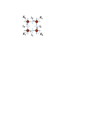
Consider first the coefficients of the box integrals. We obtain them from the quadruple cut shown in fig. 2. The cut propagators correspond to the four propagators of the desired box coefficient. As observed in ref. BCFUnitarity , if we take the loop momentum to be four-dimensional, then the four cut conditions,
| (4) |
match the number of components of the loop momentum, leading to a discrete sum over two solutions for . The integration is effectively frozen. The are the masses of the particles in the cut propagators, which in this paper are taken to vanish. The coefficient of any box integral is then given in terms of a product of four tree amplitudes,
| (5) | |||||
| (6) |
where the sum runs over the two solutions to the on-shell conditions, labeled by “” and “”. The four tree amplitudes in eq. (6) correspond to the tree amplitudes at the four corners of the quadruple cut depicted in fig. 2.
The generic solution for was found in ref. BCFUnitarity . Simpler forms can be found for particular, but still fairly general, kinematical cases. In this paper, we focus on the case of massless particles circulating in the loop. When in addition at least one external leg, say leg 1, of the box integral shown in fig. 2 is also massless, that is , the two solutions to the on-shell conditions (4) can be written in a remarkably simple form,
| (7) |
As illustrated in fig. 2, the are the external momenta of the corners of the box integral under consideration and and are Weyl spinors corresponding to the massless momentum , in the notation of refs. TreeReview . In massless QCD this solution covers all helicity configurations for amplitudes with up to seven external quarks or gluons, and a large fraction of the box coefficients for more external partons. (This solution may also be found in Risager’s Ph.D. thesis RisagerThesis .)
The solution (7) has the advantage of making it manifest that Gram determinants enter only as square roots, one for each power of loop momenta in the numerator of box integrals. Indeed, the Gram determinant is given by the product of the spinor-product strings in the denominators of eq. (7),
| (8) |
where , , is the box Gram determinant for . This property reduces the severity of numerical round-off error due to cancellations between different terms, in the regions of phase space where the Gram determinant vanishes.
II.2 Triangle Coefficients from Discrete Fourier Projection
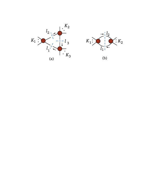
To evaluate the coefficients of the triangle and bubble integrals, we make use of elements from the approaches of both OPP OPP and Forde Forde . First consider the triangle integrals. To obtain the coefficients in eq. (2) we use the triple cut depicted in fig. 3(a). In contrast to the quadruple cut, the triple cut does not freeze the integral, but leaves one degree of freedom which we denote by . Moreover, the triple cut also contains box integral contributions. This makes the extraction of the triangle coefficients somewhat more intricate than the box coefficients.
For massless internal particles, the solution of the cut condition () is AguilaPittau ; OPP ; Forde
| (9) |
and, using momentum conservation, , . Here is a complex parameter corresponding to the one component of the loop momentum not fixed by the cut condition. Following ref. Forde we have,
| (10) |
with , , and and are both massless. (In comparison with ref. Forde , we have rescaled and relabeled these massless momenta, and here we take all external momenta to be outgoing.) The variables , and are defined as follows,
| (11) |
where
| (12) |
with running over (or any other pair). To determine the coefficients of integrals we must sum over the two solutions corresponding to and . It turns out that for the three-external-mass case, these solutions are related by taking . In addition, when a corner of the triangle is massless, simpler forms of the solutions can be obtained. These issues will be discussed elsewhere Future . A similar solution to eq. (9) has been given in the massive case KilgoreCut .
OPP OPP showed that after subtracting the known box contributions from the triple cut integrand, one is left with seven independent coefficients. One of these seven corresponds to the coefficient of the scalar triangle we seek, while the remaining six correspond to terms that integrate to zero. Evaluating the subtracted triple-cut integrand at seven selected kinematic points leads to a system of linear equations for these coefficients. As discussed in ref. EGK , however, numerical stability issues can arise from inverting this linear system of equations. The OPP approach of solving a system of equations is currently being implemented in numerical programs, with initial results reported in refs. EGK ; CutTools ; GKM ; OPP2 ; NLMLesHouches ; MOPP . In the alternative approach of Forde Forde , the coefficient is instead extracted from the analytic behavior of the triple cut in the limit that the complex variable becomes large.
We choose to use a hybrid of these approaches, subtracting box contributions from the triple cuts following OPP, but in a way that makes manifest the analytic properties in the complex variable following Forde. The triple cut is,
| (13) |
Each of the box contributions to the triple cut (13) contains a fourth Feynman propagator, for some . Hence develops a pole in whenever the inverse propagator vanishes, say
| (14) |
The pole locations and coefficients are determined from the form of , after inserting the triple-cut loop momentum parametrization (9).
The residues at the poles also involve the coefficients of the box integral, evaluated on the two solutions to the quadruple cuts. The can be computed prior to the triangle calculation, and their contribution subtracted to form the difference,
| (15) |
Equation (15) is slightly schematic, omitting a few subtleties that depend in part on how many of the triangle legs are massive. For example, in the three-mass case we should either sum over and , or else make use of the relation between the two triple-cut solutions to eliminate one of them Future . The main point is that proper subtraction of the box contributions removes all poles at finite values of , so that has poles only at and , as sketched in fig. 4. Thus we can write,
| (16) |
From eq. (9) we see that the maximum power of in eq. (16), denoted by , is equal to the maximum tensor rank encountered at the level of triangle integrals. In a generic renormalizable theory such as QCD, this value is .
As explained in ref. Forde , the desired coefficient of the triangle integral is given by , which can be extracted by taking the limit and keeping only the contribution. This “Inf” operation can be applied to either or the box-subtracted triple cut integrand , because the box contributions vanish as . In the language of OPP, the terms with in eq. (16) correspond to terms that integrate to zero.
We can also express the triangle coefficient using a contour integral around ,
| (17) |
as depicted in fig. 4. However, because of the special analytic form (16) of , it is much more efficient numerically to evaluate this contour integral by means of a discrete Fourier projection,
| (18) |
where is an arbitrary complex number. This projection removes the remaining coefficients , . As it turns out, we do need the other coefficients in order to subtract out triangle contributions when evaluating bubble coefficients Future . We can obtain them from the same evaluations of , by multiplying or dividing by factors of before carrying out the Fourier sum,
| (19) |
As we shall discuss in section IV, the discrete Fourier projection provides excellent numerical stability.
II.3 Bubble Coefficients
Next consider the bubble coefficients. To parametrize the remaining degrees of freedom left by the two-particle cuts shown in fig. 3(b), we make use of a lightlike vector constructed from the external momentum and an arbitrary lightlike vector . The associated spinors are and . The normalization of is determined by the constraint that , which ensures that
| (20) |
is lightlike. Note that this definition of differs from the one (10) in the triangle discussion, and is used exclusively for the two-particle cuts associated with the bubble coefficient. The cut conditions () are solved by the momenta,
| (21) |
In the two-particle cuts it is sometimes useful to restrict the cut loop momenta to be real. In this case, for , the cut corresponds to a physical rescattering process. It is convenient to view the rescattering in the center-of-mass frame, in which , the energies of the intermediate momenta are fixed to be , and the phase space can be parametrized alternatively by the polar and azimuthal angles and for one of the two momenta, say . The relation between the two parametrizations is given by,
| (22) |
Then is real and restricted to , while with .
After subtracting box and triangle contributions from the two-particle cut under consideration OPP ; EGK ,
| (23) |
we are left with a tensorial expression in terms of the loop momentum , with maximal rank . (In general, if the maximal rank of the triangle integrals is , the maximal rank of bubble integrals is .) In terms of the parametrization (21), is a order polynomial expression in terms of the monomials , and . The bubble coefficient is then given by the integral Future ,
| (24) |
The factor of is a Jacobian for the change of variables (22) from to .
As in the case of the triangle coefficients, the special analytic form of the subtracted two-particle cut allows the integral (24) to be evaluated efficiently using a discrete Fourier projection. Two observations are important here: the integration projects onto the terms independent of , which are of maximal power in ; also, the integration amounts to replacing positive powers of by rational numbers Forde . Following similar logic as in the triangle case, we can extract the bubble coefficient with a double discrete Fourier projection on the subtracted two-particle cut,
| (25) |
where and are arbitrary complex constants. For the case , we use the fact that for , the desired combination can be written as . In this way it is possible to reduce the number of values of required, from three in eq. (25) to two:
| (26) |
One can also reduce the number of values of sampled, from five down to three or four, using lower-order roots of unity (independently of how is treated). In a similar fashion to eq. (19), higher-rank tensor bubble coefficients may be extracted by weighting the sum (25) differently. (Such coefficients would feed into the calculation of tadpole coefficients. They are not needed for the case of massless internal lines treated in this paper.)
Due to the physical interpretation of the two-particle cut as a rescattering, with real intermediate momenta living on a sphere, an alternative projection formula from eqs. (25) and (26) may be found in terms of spherical harmonics . To do so we change from the variables and to the spherical coordinates and via eq. (22). In these variables, the loop momentum (21) is linear in the spherical harmonics with and , because
| (27) |
The two-particle cut with box and triangle contributions subtracted is then a superposition of spherical harmonics,
| (28) |
The scalar bubble coefficient is just , up to a normalization constant. Using eq. (21), the higher spherical-harmonic coefficients can be related to the coefficients of the higher-rank tensor integrals.
III Rational Contributions
We now turn to the question of computing the rational terms in the amplitude (1). Here we use the on-shell recursive approach for one-loop amplitudes Bootstrap ; Genhel , modifying it to make it more amenable to numerical evaluation in an automated program. As is true for the cut parts, an important feature of on-shell recursion is that it displays a modest growth in computational resource requirements — compared to the rapid growth with a traditional Feynman-diagram approach — as the number of external particles increases.
At one loop, as at tree level, on-shell recursion provides a systematic means of determining rational functions, using knowledge of their poles and residues. At loop level, however, a number of new issues must be addressed, including the appearance of branch cuts, spurious singularities, and the behavior of loop amplitudes under large complex deformations. In some cases, “unreal poles” develop DoublePole , which are poles present with complex but not real momenta. The appearance of branch cuts does not present any difficulties because we use on-shell recursion only for the cut-free rational remainders . As noted in ref. Genhel , we can sidestep the problems of unreal poles by choosing appropriate shifts within the class given below in eq. (29). Finally, we may determine the behavior of amplitudes under large complex deformations by using auxiliary recursion relations.
III.1 General Principles
On-shell recursion relations may be derived by considering deformations of amplitudes characterized by a single complex parameter , such that all external momenta are left on shell BCFW . In the massless case, it is particularly convenient to shift the momenta of two external legs, say and ,
| (29) | |||||
We denote the shift in eq. (29) as a shift. This shift has the required property that the momentum conservation is left undisturbed, while shifted momenta are left on-shell, .
On-shell recursion relations follow from evaluating the contour integral,
| (30) |
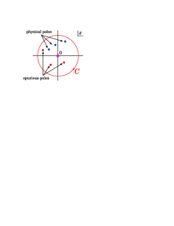
where the contour is taken around the circle at infinity, as depicted in fig. 5, and is evaluated at the shifted momenta (29). If the rational terms under consideration vanish as , the contour integral vanishes and Cauchy’s theorem gives us a relationship between the desired rational contributions at , and a sum over residues of the poles of , located at ,
| (31) |
On the other hand, if the amplitude does not vanish as , there are additional contributions, which we can obtain from an auxiliary recursion relation Genhel .

Poles in the -shifted one-loop rational terms, labeled by in eq. (31), may be separated into two classes as shown in fig. 5: physical and spurious. The physical poles are present in the full amplitude , and correspond to genuine, physical factorization poles (collinear or multiparticle). The spurious poles are not poles of ; they cancel between the cut parts and rational parts . They arise from the presence of tensor integrals in the underlying field-theory representation of the amplitude. Our method avoids the need to perform the reduction of such tensor integrals explicitly, because of the use of a basis of master integrals. The reduction happens implicitly, and leaves its trace in the presence of Gram determinant denominators. These denominators give rise to spurious singularities in individual terms. Separating the different contributions, we may write,
| (32) |
where contains all contributions from physical poles, the contributions from spurious poles, and the possible contributions from large deformation parameter , if does not vanish there. More explicitly, from elementary complex variable theory, under the shift (29) the rational terms can be expressed as a sum over pole terms and possibly a polynomial in ,
| (33) | |||||
where the coefficients are functions of the external momenta. The poles in in eq. (33) are shown in fig. 5. The physical poles labeled by are generically single poles. (Some shift choices may lead to double poles DoublePole ; we can generally avoid such shifts Genhel .) In general, in a renormalizable gauge theory, the spurious poles, labeled by , may be either single or double poles Future . If vanishes for large , the are all zero. If not, then gives a contribution to the physical rational terms, .
The contributions of the physical poles may be obtained efficiently using the on-shell recursive terms represented by the diagrams in fig. 6. The tree “vertices” labeled by “” denote tree-level on-shell amplitudes , while the loop vertices “”are the rational parts of on-shell (lower-point) one-loop amplitudes , , as defined in eq. (3). The contribution in fig. 6(c) involves the rational part of the additional factorization function BernChalmers . It only appears in multi-particle channels, and only if the tree amplitude contains a pole in that channel. Each diagram is associated with a physical pole in the plane, illustrated in fig. 5, whose location is given by,
| (34) |
where . This pole arises from the vanishing of shifted propagators, . Generically the sum over is replaced by a double sum over , labeling the recursive diagrams, where legs labeled and always appear on opposite sides of the propagator in fig. 6. The computation of the recursive diagrams has been described in refs. Bootstrap ; OneLoopMHV ; OnShellReview , to which we refer the reader for further details.
What about the contributions of the spurious poles? One approach is to find a “cut completion” Bootstrap ; Genhel , which is designed by adding appropriate rational terms to in order to cancel entirely the spurious poles in within the redefined cut terms . Because the complete amplitude is free of the spurious poles, this procedure ensures that the redefined rational terms are free of them. The cut completion makes it unnecessary to compute residues of spurious poles (although additional “overlap” diagrams are introduced). It is very helpful for deriving compact analytic expressions for the amplitudes. This approach has led to the computation of the rational terms for a variety of one-loop MHV amplitudes with an arbitrary number of external legs Bootstrap ; OtherBootstrap ; Genhel , as well as for six-point amplitudes. In general, it should be possible to construct a set of cut completions using integral functions of the type given in ref. CGM to absorb spurious singularities.
For the purposes of a numerical program, however, it is simpler to extract the spurious residues from the known cut parts. These residues are guaranteed to be the negatives of the spurious-pole residues in the rational part. That is, the spurious contributions are,
| (35) |
where is the shifted cut part appearing in eq. (1). The spurious poles correspond to the vanishing of shifted Gram determinants, for , associated with bubble, triangle and box integrals. (In the case of massless internal propagators, the bubble Gram determinant does not generate any spurious poles.)
A simple example of a spurious singularity in the cut part (2) is from a bubble term of the form,
| (36) |
where is smooth as , and for some massless momentum . The denominator factor is the square root of the Gram determinant for a triangle integral with two massive legs, and , and one massless leg, . Under the shift, there will be a value of , , for which the shifted denominator vanishes linearly, (unless and both belong to the same massive momentum cluster, or , in which case the Gram determinant is unshifted). From eq. (35) we see that we only need the rational pieces of the spurious-pole residues of the cut part, because is rational. From eq. (36), we see that there can only be a rational piece if we have to series expand the logarithm to compute the residue. Hence the spurious pole in the bubble coefficient must be of at least second order in . At order , box and triangle integrals contain dilogarithms and squared logarithms, which must be expanded to second order to obtain a rational piece. Thus the spurious poles of box and triangle coefficients must be at least of third order for rational terms to be generated.
To extract a residue from , we evaluate the integral coefficients numerically for complex, shifted momenta in the vicinity of the spurious pole, using our implementation of the results of section II. We also need to evaluate the loop integrals. First, however, we perform an analytic series expansion of the integrals around the vanishing Gram determinants. For example, the three-mass triangle integral, , close to the surface of its vanishing Gram determinant,
| (37) |
behaves as,
| (38) | |||||
where the index on the shifted invariant, , is defined mod 3. In this expression the logarithms are to be expanded according to,
| (39) |
where , and is the value of the shifted invariant at the location of the spurious pole. The leading order of eq. (38) matches the expansion found in ref. CGM . In the integral expansions we need keep only rational terms, including terms that can become rational after further series expansion around a generic point, such as eq. (39). Thus we may avoid computing any logarithms or polylogarithms at complex momentum values. The expression obtained by replacing according to these rules, in the vicinity of , will be denoted by . In ref. Future we present the complete set of integral expansions needed in the calculations, as well as a convenient method for generating them from a dimension-shifting formula BDKIntegrals .
III.2 Discrete Fourier Sum for Spurious Residues
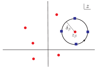
Similarly to the case of triangle and bubble coefficients, we extract each required spurious-pole residue from the cut parts by using a discrete Fourier sum. We evaluate at points equally spaced around a circle of radius in the plane, centered on the pole location , as depicted in fig. 7; i.e., , for . In contrast to the -plane analysis used earlier to obtain triangle coefficients, however, we do not know the residues at other poles a priori, so we cannot subtract them easily. (Indeed, the function we are analyzing is only rational in the vicinity of , due to our use of the rational parts of the integral expansions around this point.) Here the discrete Fourier sum is an approximation to the contour integral, whereas in the previous section it was exact. We can make the approximation arbitrarily accurate in principle, by choosing to be arbitrarily small. With finite precision, however, numerical round-off error forces us to work at finite . When extracting the residue of a spurious pole we must also ensure that there are no other poles inside or near the circle. To obtain the contributions of the spurious poles to in eq. (35) we evaluate,
| (40) |
The sum over runs over the location of all spurious Gram determinant poles that contribute to rational terms. Equivalently, we can extract the coefficients and in eq. (33) via,
| (41) |
For the results presented in the next section we choose points in the discrete sum. In general, an increase in increases the precision, but at the cost of computation time.
We choose to be much smaller than the distance to nearby poles, but not so small as to lose numerical precision. Typically at “standard” double precision we use a value of . If the contributions from the nearby poles are unusually large, then we find a large variation in the absolute value of each term in the sum. If this happens we reduce until either the variation is acceptable, or we cross a minimum value of , beyond which the point becomes unstable because of round-off error. We deal with such points as described below.
III.3 Numerical Stability
In addition to the value of becoming too small, other cancellations can also sometimes cause a loss of precision, giving rise to a potentially unstable kinematic point. In order to identify such phase-space points more generally, we apply consistency checks independently to the cut and rational parts of the amplitude. For the cut part we test how well the known, non-logarithmic singularities are reproduced. Because the only source of such poles are the bubble integrals, for the -gluon amplitudes, for example, we have GG ; KST ,
| (42) |
where is the number of quark flavors and the sum on runs over all bubble integrals. As a practical matter it is sufficient to check that the divergent term divided by the tree amplitude is real. (For helicity configurations with vanishing tree amplitudes the cut contributions vanish, so no check is required.) Because bubble coefficients are computed from expressions where triangle and box contributions have been subtracted, any instabilities in the latter are also detected with this consistency check.
In general this test is not sufficient for finding all the unstable points of the full amplitude, because some of the instability comes from computing the spurious residues for rational terms. A related test, which suffices to find all remaining instabilities, comes from the requirement that each spurious singularity must cancel in the sum over bubble coefficients. This cancellation can be understood by applying the shift to eq. (42), and making use of the fact that has no spurious poles. For each spurious-pole residue that contributes to the rational part, we therefore check that the sum of discrete Fourier sums over all bubble coefficients,
| (43) |
vanishes to within a specified tolerance.
If a phase-space point fails the above stability conditions we recalculate the point in a manner that improves its stability. Various strategies have been proposed in the literature to handle unstable points. One approach is to modify the standard integral basis (2) so as to absorb the Gram determinant singularities into well-defined functions FiveGluon ; Zqqgg ; CGM ; Denner ; Binoth . This approach is related to using a cut completion Bootstrap . Other approaches are to interpolate across the singular region or to series expand the integrals in the singular region GramInterpolate ; Denner . A third approach is to simply redo unstable points at higher precision, e.g. as in ref. CutTools .
We have found the high-precision approach to be effective for eliminating the remaining instabilities in our program. It is robust and simple to implement; a detailed analysis of the instabilities is not needed, and we can use the standard basis of integrals with no interpolations or expansions of the integrals around unstable points. Our implementation of on-shell methods already has only a small fraction of unstable phase-space points; hence the overhead of recomputing them at higher precision is relatively small. We use the QD package QD , switching to “double-double” precision, that is approximately 32 decimal digits. If the stability test were to fail at this level of precision, we switch to “quadruple-double” precision, corresponding to approximately 64 digits of precision; for all amplitudes calculated here, this happens rarely, if ever. To compute the integrals to higher precision, we implement the polylogarithms which enter the integrals using a series expansion to a sufficiently high order. If the test (42) fails then we recompute the entire cut part at higher precision, but if the spurious-pole test (43) fails we only recompute those pieces containing unstable Gram determinant singularities.
Further details, as well as all integral expansions used to extract the spurious residues from the cut part, will be given elsewhere Future .
IV Results
We now discuss the numerical stability of our implementation. Our stability tests use sets of 100,000 points for gluon scattering, generated with a flat phase-space distribution using the RAMBO RAMBO algorithm. We impose kinematic cuts on the outgoing gluons, following ref. EGK :
| (44) |
where is the gluon transverse energy, is the pseudorapidity, and is the separation cut between pairs of gluons. The center-of-mass energy is chosen to be TeV and the scale parameter (arising from divergent loop integrals) is set to TeV.
We computed one-loop six-, seven- and eight-gluon amplitudes for with BlackHat at each phase-space point, and compared the output against a target expression, obtained either from known analytic results, or from BlackHat itself using quadruple-double precision ( digits). As an additional test, we also used ordinary double precision to compare to the numerical results of refs. EGZ ; GKM at the quoted phase-space points. We find agreement for the five- and six-gluon amplitudes for all helicity configurations, to within their quoted accuracy, after accounting for external phase conventions and the incoming-particle convention implicitly used in ref. GKM . We also find agreement with the numerical results of ref. Genhel at the quoted phase-space points for the six-, seven- and eight-point maximally helicity violating (MHV) amplitudes presented here.
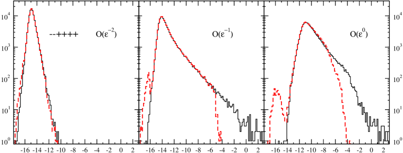
The histograms in figs. 8–10 show the results of our study of numerical precision. For these plots, the horizontal axis is the logarithmic relative error,
| (45) |
for each of the , and components of the numerical amplitude obtained from BlackHat. The vertical axis in these plots shows the number of phase-space points in a bin that agree with the target to a specified relative precision. We use a logarithmic vertical scale to visually enhance the tail of the distribution, so as to illustrate the numerical stability.
For the MHV amplitudes in figs. 8 and 9, we used analytic expressions from refs. UnitarityMethod ; Fusing ; Bootstrap ; OneLoopMHV as the target expressions . For the next-to-MHV (NMHV) amplitudes, analytic expressions are available Fusing ; BCFCutConstructible ; XYZ ; Genhel , although for fig. 10, we generated the target with BlackHat, using quadruple-double precision. This is more than sufficient to ensure numerical stability in target expressions for the purposes of the comparison. We note that the ability to switch easily to higher precision is quite helpful in assessing numerical stability in any new calculation.
First consider the MHV six-point amplitude . Fig. 8 illustrates the numerical stability of BlackHat for this amplitude, with and without the use of higher precision on the points identified as unstable. The plots show the distribution of relative errors for the , and components over 100,000 phase-space points. The distribution has extremely small errors, peaking at a relative error of nearly , while the right-side tail falls rapidly. For the and finite components the peaks shift to the right, to a relative precision of around and , and fall less steeply. This feature is not surprising, because of the larger number of computational steps needed for these parts of the amplitudes: for terms, only box coefficients contribute (for this helicity pattern triangle integrals do not appear); for the contribution, bubble coefficients contribute too; for the finite part, rational terms contribute as well. As one proceeds from box to triangle, bubble, and then to rational terms, each step relies on previous steps, and so numerical errors accumulate.
In each plot in fig. 8 the solid (black) curve corresponds to the exclusive use of ordinary double precision (16 decimal digits), showing good stability for the raw algorithm for all three components. The dashed (red) curve shows the effect of turning on higher precision for contributions identified as unstable, using the criteria discussed in section III. This completely suppresses the already-small tail above a relative error of about . The points populating the right-hand tail in the ordinary double precision calculation, displayed in the solid (black) curve, then move to the left in the dashed (red) curve, giving rise to a secondary peak around a relative error of machine precision, or . (The comparison with the target is performed in ordinary double-precision, even though higher precision is used in intermediate steps.) This twin-peak feature is visible in the and components. It is due our recalculation of the entire cut part, at higher precision, whenever a phase-space point fails the consistency check (42). When the spurious-pole stability test (43) fails, the point generally falls to the right of the secondary peak, because we only recalculate those pieces that contain the unstable spurious singularity.
Another important feature that can be observed in fig. 8 is that the “effective cutoff” is sharp: for the terms almost no points below are identified as unstable. In a practical calculation, given Monte-Carlo integration errors and other uncertainties, a cutoff in the relative error of is overly stringent. It does, however, illustrate the control over instabilities achieved in BlackHat, which becomes more important for more complicated processes. It is interesting to note that modest additional computation time is required to achieve a cutoff of , compared to, say, .
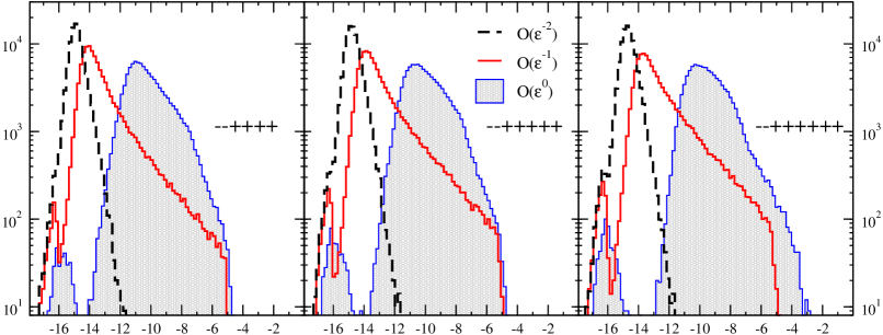
Next consider the behavior as the number of external gluons increases. In fig. 9 we show relative error distributions for the set of MHV amplitudes , and . For each of these amplitudes the dashed (black) curve shows the relative error in the coefficient of the singularity. Similarly, the relative errors in the and contributions are given by the solid (red) curve and shaded (blue) distribution. The relative precision of the singularities is better than for these six-, seven- and eight-point amplitudes. The computational-stability scaling properties in going from six- to seven- and then eight-point amplitudes in fig. 9 are also rather striking. There is little change in the shape of the curves as we increase the number of legs.
| helicity | cut part | full amplitude | full amplitude |
|---|---|---|---|
| double prec. only | with multi-prec. | ||
| 2.4 ms | 7 ms | 11 ms | |
| 4.2 ms | 11 ms | 23 ms | |
| 6.1 ms | 29 ms | 43 ms | |
| 3.1 ms | 18 ms | 32 ms | |
| 3.3 ms | 61 ms | 96 ms | |
| 4.4 ms | 12 ms | 22 ms | |
| 5.9 ms | 47 ms | 64 ms | |
| 7.0 ms | 72 ms | 114 ms |
Even more striking is the modest increase in computation time. As mentioned earlier, the tree-like nature of on-shell methods leads us to expect only mild scaling for a given helicity pattern, in stark contrast with the rapid increase in required computational resources for ordinary Feynman diagrams. These expectations are borne out by the values for the average computation time shown in Table 1. The table shows the average time on a 2.33 GHz Xeon processor for computing a color-ordered amplitude of a given helicity configuration at a single phase-space point. The first three rows show the timing for the six-, seven- and eight-point MHV amplitudes corresponding to fig. 9. Even for the eight-point case we obtain an average evaluation time of less than 50 ms, including running the phase-space points marked as unstable at higher precision. It is also interesting to note the relatively modest increase in computation time due to turning on higher precision for unstable points, even in this initial implementation. (The time in the third column includes the evaluation of bubble coefficients used in the spurious-pole test (43).)
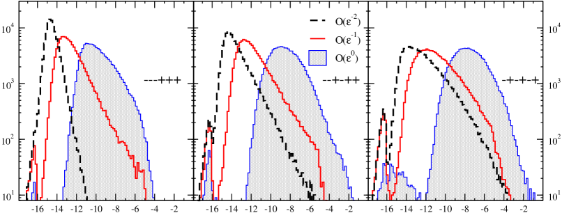
Finally, consider the six-gluon NMHV amplitudes. Figure 10 illustrates the numerical stability properties of the complete set of independent six-gluon NMHV amplitudes not related by symmetries, , and , compared against a quadruple-precision target computed with BlackHat. For each one of these amplitudes, the contributions to the , and finite terms are shown in a similar format as the MHV case. These NMHV curves are all shifted to the right compared to the MHV cases in in fig. 9. This property is not surprising; it is due to the more complicated nature of the NMHV amplitudes. In particular, the amplitudes contain higher powers of the box Gram determinants in denominators of the box coefficients, which then feed into triangle, bubble and rational contributions. As in the MHV cases, when one goes from to to , the curves shift to the right again, reflecting the more complicated calculations. Nevertheless, they all exhibit excellent numerical stability, with the distributions of relative errors for the finite pieces peaking at or better. We identify points as unstable, and automatically recompute such points at higher precision, using the same criteria as for the MHV amplitudes. In the NMHV case, the fall-off is not as sharp as in the MHV case. Nevertheless, the accuracy obtained is more than sufficient for use in an NLO program.
The average evaluation time in the current version, for all independent six-gluon helicity configurations needed at NLO, including the NMHV ones, is given in Table 1. One can see that alternating-helicity configurations do take longer to compute. However, in all cases the cut parts are evaluated in under 8 ms and the full amplitudes in under 120 ms. Although we have not run systematic tests of NMHV amplitudes beyond six points, initial studies at seven points indicate that the scaling behavior of the NMHV amplitudes is not quite as good as for the MHV case, but still very good.
V Conclusions
In this paper we presented the first results from BlackHat, an automated implementation of on-shell methods, focusing on the key practical issues of numerical stability and computational time. We illustrated the numerical stability by computing a variety of complete six-, seven- and eight-gluon helicity amplitudes and comparing the results against previously-obtained analytic results or against higher precision calculations. In this initial version we achieved reasonable speed, an average computation time of 114 ms per phase-space point for the most complicated of the six-gluon helicity amplitudes, and substantially better for the simpler helicities. We expect this speed and stability to be sufficient for carrying out phenomenological studies of backgrounds at the LHC, even as we expect further improvements with continuing optimization of the code. After the code is stable and tested for a wide variety of processes, we plan to make it publicly available.
BlackHat uses the unitarity method with four-dimensional loop momenta UnitarityMethod ; Fusing . This method allows the use of compact tree-level helicity amplitudes as the basic building blocks. We compute the box coefficients using quadruple cuts BCFUnitarity . For box integrals with massless internal propagators and at least one massless corner, we presented a simple solution to the cut conditions. The solution makes manifest the presence of square roots, rather than full powers, of a spurious (Gram determinant) singularity for each power of the loop momentum in the numerator. We evaluated the triangle- and bubble-integral coefficients using Forde’s approach Forde to expose their complex-analytic structure. Another important ingredient in our procedure is the OPP OPP subtraction of boxes from triple cuts when computing triangle coefficients, and of boxes and triangles from ordinary (double) cuts when computing bubble coefficients. Viewed in terms of Forde’s complex-valued parametrization approach, the OPP subtraction cleans the complex plane of poles, using previously-computed coefficients. We then introduced a discrete Fourier projection, as an efficient and numerically stable method for extracting the desired coefficients. In the bubble case, this procedure can be recast in terms of spherical harmonics.
We computed the purely rational terms using loop-level on-shell recursion, modifying the treatment of spurious singularities compared to refs. Bootstrap ; Genhel . We used a discrete Fourier sum to compute the spurious-pole residues from the cut parts. These contributions are then subtracted from the recursively-computed rational terms in order to cancel spurious singularities implicit in the latter, and thereby make the full amplitude free of spurious singularities as required.
The computation of most points in phase space proceeds using ordinary double-precision arithmetic to an accuracy of or less. This is far better than the Monte-Carlo integration errors that will inevitably arise in any use of amplitudes in an NLO parton-level or parton-shower code (not to mention parton distribution, scale, shower and hadronization uncertainties). Nonetheless, the computation of the amplitude at a small percentage of phase-space points does manifest a loss of precision, resulting in an instability and larger error. In order to identify such unstable points as may arise, we impose the requirements that all spurious singularities cancel amongst bubble coefficients, and that the coefficients of the singularity (corresponding to -singular terms in bubble integrals) be correct. Whenever the calculation at a given phase-space point fails these criteria we simply recalculate the point at higher precision. There are other possible means for dealing with Gram-determinant singularities FJT ; OtherGramMethods ; GramInterpolate ; Denner ; NLMLesHouches , but we prefer this approach because of its simplicity CutTools . In practice, it has a relatively modest impact on the overall speed of the program. In the most complicated of the six-gluon helicity amplitudes, higher-precision evaluation causes the time to increase modestly, from 72 ms to 114 ms. We expect to see further improvements with additional refinements.
It is important to validate a numerical method against known analytic results. For this purpose, we made use of MHV configurations, which contain two gluons of helicity opposite to that of the others. In particular, we considered the case where the two opposite helicities are nearest neighbors in the color order. In earlier work, these amplitudes were computed for an arbitrary number of external gluons Bootstrap ; OneLoopMHV , using on-shell methods. We used these results to confirm that BlackHat returns the correct values through eight gluons. We also verified numerical stability for non-MHV amplitudes by comparing results for all six-gluon amplitudes against a reference computation done entirely using quadruple-precision arithmetic.
We defer discussion of amplitudes with external fermions, or with massive quarks and vector bosons, to the future. (Some work directly relevant to the question of adding massive particles may be found in refs. Massivetree ; BFMassive ; KilgoreCut .) We will also present further details, including the integral expansions we use around spurious singularities, in a future publication Future .
The excellent numerical stability and timing performance of BlackHat is due to a variety of ideas described in this paper. Because the unitarity method uses gauge-invariant tree amplitudes as the basic input into the calculation, we avoid the large gauge cancellations inherent in Feynman-diagram calculations. In addition we made use of very compact four-dimensional tree-level helicity amplitudes as the basic input to the calculations. All steps in our computation of the rational terms, as well as the integral coefficients, are carried out in four dimensions. Our simple quadruple-cut solution (7) also helps maintain numerical stability in the box contributions. Our parametrization choices for triple and double cuts, and the OPP subtraction of previously-computed coefficients are additional important ingredients. Finally, our use of discrete Fourier projections helps considerably.
The resulting C++ code BlackHat is efficient and numerically stable, as we have illustrated with the computation of various one-loop gluon amplitudes and their comparison to known analytic expressions. Based on the results presented here, we expect BlackHat to make possible the computation of a wide variety of new one-loop amplitudes for collider physics that have been inaccessible with traditional methods. We hope that BlackHat, in conjunction with automated programs GK for combining the real and virtual contributions at NLO, will soon enable the computation of phenomenologically important cross-sections at the LHC.
Acknowledgments
We would like to thank John Joseph Carrasco, Tanju Gleisberg, Henrik Johansson and Michael Peskin for helpful discussions. We are grateful to the Galileo Galilei Institute for Theoretical Physics for hospitality while part of this work was carried out. We also thank Academic Technology Services at UCLA for computer support. This research was supported by the US Department of Energy under contracts DE–FG03–91ER40662 and DE–AC02–76SF00515. CFB’s research was supported in part by funds provided by the U.S. Department of Energy (D.O.E.) under cooperative research agreement DE-FC02-94ER40818, and in part by the National Science Foundation under Grant No. PHY05-51164. DAK’s research is supported by the Agence Nationale de la Recherce of France under grant ANR–05–BLAN–0073–01. The work of DM was supported by the Swiss National Science Foundation (SNF) under contract PBZH2-117028.
References
- (1) Z. Bern et al., 0803.0494 [hep-ph].
-
(2)
C. Anastasiou, L. J. Dixon, K. Melnikov and F. Petriello,
Phys. Rev. D 69, 094008 (2004)
[hep-ph/0312266];
K. Melnikov and F. Petriello, Phys. Rev. Lett. 96, 231803 (2006) [hep-ph/0603182]; Phys. Rev. D 74, 114017 (2006) [hep-ph/0609070];
S. Frixione and M. L. Mangano, JHEP 0405, 056 (2004) [hep-ph/0405130];
N. E. Adam, V. Halyo and S. A. Yost, 0802.3251 [hep-ph]. -
(3)
R. V. Harlander and W. B. Kilgore,
Phys. Rev. Lett. 88, 201801 (2002)
[hep-ph/0201206];
C. Anastasiou and K. Melnikov, Nucl. Phys. B 646, 220 (2002) [hep-ph/0207004];
C. Anastasiou, K. Melnikov and F. Petriello, Phys. Rev. Lett. 93, 262002 (2004) [hep-ph/0409088];
Nucl. Phys. B 724, 197 (2005) [hep-ph/0501130];
G. Davatz et al., JHEP 0607, 037 (2006) [hep-ph/0604077];
C. Anastasiou, G. Dissertori, F. Stöckli and B. R. Webber, JHEP 0803, 017 (2008) [0801.2682 [hep-ph]]. - (4) A. Denner, S. Dittmaier, M. Roth and L. H. Wieders, Phys. Lett. B 612, 223 (2005) [hep-ph/0502063]; Nucl. Phys. B 724, 247 (2005) [hep-ph/0505042].
- (5) A. Denner and S. Dittmaier, Nucl. Phys. B 734, 62 (2006) [hep-ph/0509141].
- (6) W. T. Giele and E. W. N. Glover, Phys. Rev. D 46, 1980 (1992).
-
(7)
W. T. Giele, E. W. N. Glover and D. A. Kosower,
Nucl. Phys. B 403, 633 (1993)
[hep-ph/9302225];
S. Frixione, Z. Kunszt and A. Signer, Nucl. Phys. B 467, 399 (1996) [hep-ph/9512328]. - (8) S. Catani and M. H. Seymour, Phys. Lett. B 378, 287 (1996) [hep-ph/9602277]; Nucl. Phys. B 485, 291 (1997) [Erratum-ibid. B 510, 503 (1998)] [hep-ph/9605323].
-
(9)
T. Gleisberg and F. Krauss,
Eur. Phys. J. C 53, 501 (2008)
[0709.2881 [hep-ph]];
M. H. Seymour and C. Tevlin, 0803.2231 [hep-ph]. -
(10)
Z. Kunszt, A. Signer and Z. Trócsányi,
Nucl. Phys. B 420, 550 (1994)
[hep-ph/9401294];
S. Catani, Phys. Lett. B 427, 161 (1998) [hep-ph/9802439]. -
(11)
F. A. Berends, R. Kleiss, P. De Causmaecker, R. Gastmans and T. T. Wu,
Phys. Lett. B 103, 124 (1981);
P. De Causmaecker, R. Gastmans, W. Troost and T. T. Wu, Nucl. Phys. B 206, 53 (1982);
Z. Xu, D. H. Zhang and L. Chang, TUTP-84/3-TSINGHUA;
R. Kleiss and W. J. Stirling, Nucl. Phys. B 262, 235 (1985);
J. F. Gunion and Z. Kunszt, Phys. Lett. B 161, 333 (1985);
Z. Xu, D. H. Zhang and L. Chang, Nucl. Phys. B 291, 392 (1987). -
(12)
A. Denner and S. Dittmaier,
Nucl. Phys. B 658, 175 (2003)
[hep-ph/0212259];
Z. Nagy and D. E. Soper,
JHEP 0309, 055 (2003)
[hep-ph/0308127];
Phys. Rev. D 74, 093006 (2006)
[hep-ph/0610028];
W. T. Giele and E. W. N. Glover, JHEP 0404, 029 (2004) [hep-ph/0402152];
R. K. Ellis, W. T. Giele and G. Zanderighi, Phys. Rev. D 72, 054018 (2005) [Erratum-ibid. D 74, 079902 (2006)] [hep-ph/0506196]; Phys. Rev. D 73, 014027 (2006) [hep-ph/0508308];
C. Anastasiou and A. Daleo, JHEP 0610, 031 (2006) [hep-ph/0511176];
A. Brandhuber, B. Spence and G. Travaglini, JHEP 0702, 088 (2007) [hep-th/0612007];
A. Lazopoulos, K. Melnikov and F. Petriello, Phys. Rev. D 76, 014001 (2007) [hep-ph/0703273];
A. Brandhuber, B. Spence, G. Travaglini and K. Zoubos, JHEP 0707, 002 (2007) [0704.0245 [hep-th]];
M. Moretti, F. Piccinini and A. D. Polosa, 0802.4171 [hep-ph]. - (13) F. del Aguila and R. Pittau, JHEP 0407, 017 (2004) [hep-ph/0404120].
- (14) T. Binoth, J. P. Guillet, G. Heinrich, E. Pilon and C. Schubert, JHEP 0510, 015 (2005) [hep-ph/0504267].
- (15) R. K. Ellis, W. T. Giele and G. Zanderighi, JHEP 0605, 027 (2006) [hep-ph/0602185].
-
(16)
Z. Xiao, G. Yang and C. J. Zhu,
Nucl. Phys. B 758, 1 (2006)
[hep-ph/0607015];
Nucl. Phys. B 758, 53 (2006)
[hep-ph/0607017];
T. Binoth, J. P. Guillet and G. Heinrich, JHEP 0702, 013 (2007) [hep-ph/0609054]. - (17) Z. Bern, L. J. Dixon, D. C. Dunbar and D. A. Kosower, Nucl. Phys. B 425, 217 (1994) [hep-ph/9403226].
- (18) Z. Bern, L. J. Dixon and D. A. Kosower, Nucl. Phys. B 513, 3 (1998) [hep-ph/9708239].
-
(19)
Z. Bern and A. G. Morgan,
Nucl. Phys. B 467, 479 (1996)
[hep-ph/9511336];
Z. Bern, L. J. Dixon and D. A. Kosower, Ann. Rev. Nucl. Part. Sci. 46, 109 (1996) [hep-ph/9602280];
Z. Bern, L. J. Dixon, D. C. Dunbar and D. A. Kosower, Phys. Lett. B 394, 105 (1997) [hep-th/9611127]. - (20) Z. Bern, L. J. Dixon and D. A. Kosower, JHEP 0001, 027 (2000) [hep-ph/0001001].
- (21) R. Britto, F. Cachazo and B. Feng, Nucl. Phys. B 725, 275 (2005) [hep-th/0412103].
-
(22)
R. Britto, F. Cachazo and B. Feng,
Phys. Rev. D 71, 025012 (2005)
[hep-th/0410179];
S. J. Bidder, N. E. J. Bjerrum-Bohr, L. J. Dixon and D. C. Dunbar, Phys. Lett. B 606, 189 (2005) [hep-th/0410296];
S. J. Bidder, N. E. J. Bjerrum-Bohr, D. C. Dunbar and W. B. Perkins, Phys. Lett. B 612, 75 (2005) [hep-th/0502028];
S. J. Bidder, D. C. Dunbar and W. B. Perkins, JHEP 0508, 055 (2005) [hep-th/0505249];
Z. Bern, N. E. J. Bjerrum-Bohr, D. C. Dunbar and H. Ita, JHEP 0511, 027 (2005) [hep-ph/0507019];
N. E. J. Bjerrum-Bohr, D. C. Dunbar and W. B. Perkins, 0709.2086 [hep-ph]. - (23) R. Britto, F. Cachazo and B. Feng, Nucl. Phys. B 715, 499 (2005) [hep-th/0412308].
- (24) R. Britto, F. Cachazo, B. Feng and E. Witten, Phys. Rev. Lett. 94, 181602 (2005) [hep-th/0501052].
- (25) Z. Bern, L. J. Dixon and D. A. Kosower, Phys. Rev. D 71, 105013 (2005) [hep-th/0501240]; Phys. Rev. D 72, 125003 (2005) [hep-ph/0505055].
- (26) Z. Bern, L. J. Dixon and D. A. Kosower, Phys. Rev. D 73, 065013 (2006) [hep-ph/0507005].
- (27) C. F. Berger, Z. Bern, L. J. Dixon, D. Forde and D. A. Kosower, Phys. Rev. D 74, 036009 (2006) [hep-ph/0604195].
-
(28)
C. F. Berger, V. Del Duca and L. J. Dixon,
Phys. Rev. D 74, 094021 (2006)
[Erratum-ibid. D 76, 099901 (2007)]
[hep-ph/0608180];
S. D. Badger, E. W. N. Glover and K. Risager, JHEP 0707, 066 (2007) [0704.3914 [hep-ph]]. -
(29)
R. Britto, E. Buchbinder, F. Cachazo and B. Feng,
Phys. Rev. D 72, 065012 (2005)
hep-ph/0503132];
R. Britto, B. Feng and P. Mastrolia, Phys. Rev. D 73, 105004 (2006) [hep-ph/0602178];
P. Mastrolia, Phys. Lett. B 644, 272 (2007) [hep-th/0611091]. - (30) A. Brandhuber, S. McNamara, B. J. Spence and G. Travaglini, JHEP 0510, 011 (2005) [hep-th/0506068].
- (31) G. Ossola, C. G. Papadopoulos and R. Pittau, Nucl. Phys. B 763, 147 (2007) [hep-ph/0609007].
-
(32)
C. Anastasiou, R. Britto, B. Feng, Z. Kunszt and P. Mastrolia,
Phys. Lett. B 645, 213 (2007)
[hep-ph/0609191];
JHEP 0703, 111 (2007)
[hep-ph/0612277];
R. Britto and B. Feng, Phys. Rev. D 75, 105006 (2007) [hep-ph/0612089]. JHEP 0802, 095 (2008) [0711.4284 [hep-ph]];
R. Britto, B. Feng and P. Mastrolia, 0803.1989 [hep-ph];
R. Britto, B. Feng and G. Yang, 0803.3147 [hep-ph]. - (33) Z. Bern, L. J. Dixon and D. A. Kosower, Annals Phys. 322, 1587 (2007) [0704.2798 [hep-ph]].
- (34) D. Forde, Phys. Rev. D 75, 125019 (2007) [0704.1835 [hep-ph]].
- (35) R. K. Ellis, W. T. Giele and Z. Kunszt, JHEP 0803, 003 (2008) [0708.2398 [hep-ph]].
- (36) G. Ossola, C. G. Papadopoulos and R. Pittau, JHEP 0803, 042 (2008) [0711.3596 [hep-ph]].
- (37) W. T. Giele, Z. Kunszt and K. Melnikov, 0801.2237 [hep-ph].
- (38) G. Ossola, C. G. Papadopoulos and R. Pittau, 0802.1876 [hep-ph].
- (39) P. Mastrolia, G. Ossola, C. G. Papadopoulos and R. Pittau, 0803.3964 [hep-ph].
-
(40)
L. D. Landau,
Nucl. Phys. 13, 181 (1959);
S. Mandelstam, Phys. Rev. 112, 1344 (1958); Phys. Rev. 115, 1741 (1959). - (41) R. J. Eden, P. V. Landshoff, D. I. Olive, J. C. Polkinghorne, The Analytic S Matrix (Cambridge University Press, 1966).
- (42) Z. Bern, L. J. Dixon, D. C. Dunbar and D. A. Kosower, Nucl. Phys. B 435, 59 (1995) [hep-ph/9409265].
-
(43)
J. Campbell and R. K. Ellis,
Phys. Rev. D 65, 113007 (2002)
[hep-ph/0202176];
J. Campbell, R. K. Ellis and D. L. Rainwater, Phys. Rev. D 68, 094021 (2003) [hep-ph/0308195]. -
(44)
D. Forde and D. A. Kosower,
Phys. Rev. D 73, 061701 (2006)
[hep-ph/0509358];
C. F. Berger, Z. Bern, L. J. Dixon, D. Forde and D. A. Kosower, Phys. Rev. D 75, 016006 (2007) [hep-ph/0607014]. - (45) W. L. van Neerven, Nucl. Phys. B 268, 453 (1986).
-
(46)
L. M. Brown and R. P. Feynman,
Phys. Rev. 85, 231 (1952);
L.M. Brown, Nuovo Cim. 21, 3878 (1961);
B. Petersson, J. Math. Phys. 6, 1955 (1965);
G. Källén and J.S. Toll, J. Math. Phys. 6, 299 (1965);
D. B. Melrose, Nuovo Cim. 40, 181 (1965);
G. Passarino and M. J. G. Veltman, Nucl. Phys. B 160, 151 (1979);
W. L. van Neerven and J. A. M. Vermaseren, Phys. Lett. B 137, 241 (1984). - (47) Z. Bern, L. J. Dixon and D. A. Kosower, Phys. Lett. B 302, 299 (1993) [Erratum-ibid. B 318, 649 (1993)] [hep-ph/9212308].
- (48) J. Fleischer, F. Jegerlehner and O. V. Tarasov, Nucl. Phys. B 566, 423 (2000) [hep-ph/9907327].
- (49) T. Binoth, J. P. Guillet and G. Heinrich, Nucl. Phys. B 572, 361 (2000) [hep-ph/9911342].
- (50) G. Duplanc̆ić and B. Niz̆ić, Eur. Phys. J. C 35, 105 (2004) [hep-ph/0303184].
-
(51)
G. ’t Hooft and M. J. G. Veltman,
Nucl. Phys. B 153, 365 (1979);
G. J. van Oldenborgh and J. A. M. Vermaseren, Z. Phys. C 46, 425 (1990);
W. Beenakker and A. Denner, Nucl. Phys. B 338, 349 (1990);
A. Denner, U. Nierste and R. Scharf, Nucl. Phys. B 367, 637 (1991);
T. Hahn and M. Pérez-Victoria, Comput. Phys. Commun. 118, 153 (1999) [hep-ph/9807565];
R. K. Ellis and G. Zanderighi, JHEP 0802, 002 (2008) [0712.1851 [hep-ph]]. - (52) Z. Bern, L. J. Dixon and D. A. Kosower, Nucl. Phys. B 412, 751 (1994) [hep-ph/9306240].
-
(53)
Z. Bern, L. J. Dixon and D. A. Kosower,
JHEP 0408, 012 (2004)
[hep-ph/0404293];
Z. Bern, V. Del Duca, L. J. Dixon and D. A. Kosower, Phys. Rev. D 71, 045006 (2005) [hep-th/0410224]. - (54) J. M. Campbell, E. W. N. Glover and D. J. Miller, Nucl. Phys. B 498, 397 (1997) [hep-ph/9612413].
- (55) V. Del Duca, W. Kilgore, C. Oleari, C. Schmidt and D. Zeppenfeld, Nucl. Phys. B 616, 367 (2001) [hep-ph/0108030].
-
(56)
A. Ferroglia, M. Passera, G. Passarino and S. Uccirati,
Nucl. Phys. B 650, 162 (2003)
[hep-ph/0209219];
W. Giele, E. W. N. Glover and G. Zanderighi, Nucl. Phys. Proc. Suppl. 135, 275 (2004) [hep-ph/0407016]. - (57) Y. Hida, X. S. Li and D. H. Bailey, http://crd.lbl.gov/~dhbailey/mpdist, report LBNL-46996.
- (58) Maplesoft, Maple User Manual, Maplesoft, 2005.
- (59) S. Wolfram, The Mathematica book, 5th edition, Wolfram Media, Inc., 2003.
- (60) D. Maître and P. Mastrolia, 0710.5559 [hep-ph].
- (61) C. F. Berger, et al., to appear.
- (62) G. Mahlon, Phys. Rev. D 49, 2197 (1994) [hep-ph/9311213].
-
(63)
M. L. Mangano and S. J. Parke,
Phys. Rept. 200, 301 (1991);
L. J. Dixon, in QCD & Beyond: Proceedings of TASI ’95, ed. D. E. Soper (World Scientific, 1996) [hep-ph/9601359]. - (64) K. Risager, U. Copenhagen Ph.D. thesis (2008).
- (65) W. B. Kilgore, 0711.5015 [hep-ph].
- (66) Z. Bern and G. Chalmers, Nucl. Phys. B 447, 465 (1995) [hep-ph/9503236].
- (67) Z. Bern, L. J. Dixon and D. A. Kosower, Phys. Rev. Lett. 70, 2677 (1993) [hep-ph/9302280].
- (68) R. Kleiss, W. J. Stirling and S. D. Ellis, Comput. Phys. Commun. 40, 359 (1986).
-
(69)
S. D. Badger, E. W. N. Glover, V. V. Khoze and P. Svrček,
JHEP 0507, 025 (2005)
[hep-th/0504159];
K. J. Ozeren and W. J. Stirling, Eur. Phys. J. C 48, 159 (2006) [hep-ph/0603071];
C. Schwinn and S. Weinzierl, JHEP 0704, 072 (2007) [hep-ph/0703021];
A. Hall, Phys. Rev. D 77, 025011 (2008) [0710.1300 [hep-ph]].