Exploring the meson spectrum with twisted mass lattice QCD

Robert G. Petrya, Derek Harnettb, Randy Lewisa,c, R. M. Woloshynd aDepartment of Physics, University of Regina, Regina, SK, S4S 0A2, Canada
bDepartment of Physics, University College of the Fraser Valley, Abbotsford, BC, V2S 7M8, Canada
cDepartment of Physics and Astronomy, York University, Toronto, ON, M3J 1P3, Canada
dTRIUMF, 4004 Wesbrook Mall, Vancouver, BC, V6T 2A3, Canada
(March 28, 2008)
Abstract

Numerical simulations with access to all possible meson quantum numbers, JPCsuperscript𝐽𝑃𝐶J^{PC}, are presented using two-flavor (up and down) quenched twisted mass lattice QCD with three different lattice spacings and four different quark masses. The connection between the quantum numbers (P𝑃P and C𝐶C) and the symmetries of the twisted mass action is discussed, as is the connection between J𝐽J and the lattice rotation group, for the 400 operators used in this study. Curve fitting of this large data set is accomplished by using an evolutionary fitting algorithm. Results are reported for conventional and exotic quantum numbers.

pacs:
12.38.Gc, 14.40.-n, 02.60.Ed

I Introduction

Although many mesons have been observed in nature, the spectrum of known mesons does not include all the states expected in Quantum Chromodynamics. Experimental searches and theoretical studies are continuing, but gaps in current knowledge leave room for new approaches. Lattice QCD is an established method for extracting numerical predictions directly from the underlying quantum field theory, but lattice explorations of the full spectrum of mesons still suffer from limitations. For reviews of both theory and experiment for light-quark mesons, see Refs. Godfrey and Napolitano (1999); Close (2002); Klempt and Zaitsev (2007).

A helpful framework for beginning the discussion of light-quark mesons is provided by the constituent quark model, where mesons are considered to be composed of a system of two bound quarks whose spins can couple to a singlet (S=0𝑆0S=0) or triplet (S=1𝑆1S=1) total spin which in turn can couple with relative angular momentum L𝐿L between the quarks to produce a total observed angular momentum J𝐽J. Using spectroscopic notation for the states LJ2S+1superscriptsubscript𝐿𝐽2𝑆1{}^{2S+1}L_{J}, one obtains the familiar list of accessible JPCsuperscript𝐽𝑃𝐶J^{PC}, as shown in Table 1.

Since in QCD gluon fields are also present, it is possible for gluonic excitations in mesons to contribute non-trivially to the observed quantum numbers of a meson. Such hybrid mesons with the same JPCsuperscript𝐽𝑃𝐶J^{PC} as conventional mesons are difficult to distinguish but, as shown in Table 1, there is a subclass of hybrid mesons, called exotic mesons, with quantum numbers unattainable in the quark model, eg. 0superscript0absent0^{--}, 0+superscript0absent0^{+-}, 1+superscript1absent1^{-+}, 2+superscript2absent2^{+-}, and 3+superscript3absent3^{-+}. These exotic mesons, for which there is yet no definitive experimental evidence, would offer a clear signature for excited gluon dynamics.

Table 1: States accessible in the constituent quark model for different total spin S𝑆S and orbital angular momentum L𝐿L labeled by spectroscopic notation LJ2S+1superscriptsubscript𝐿𝐽2𝑆1{}^{2S+1}L_{J} with corresponding JPCsuperscript𝐽𝑃𝐶J^{PC}.
      S=0𝑆0S=0 (singlet)          S=1𝑆1S=1 (triplet)
L𝐿L LJ2S+1superscriptsubscript𝐿𝐽2𝑆1{}^{2S+1}L_{J} JPCsuperscript𝐽𝑃𝐶J^{PC} LJ2S+1superscriptsubscript𝐿𝐽2𝑆1{}^{2S+1}L_{J}         JPCsuperscript𝐽𝑃𝐶J^{PC}
S𝑆S S01superscriptsubscript𝑆01~{}~{}^{1}S_{0} 0+superscript0absent0^{-+} S13superscriptsubscript𝑆13~{}~{}^{3}S_{1} 1superscript1absent1^{--}
P𝑃P P11superscriptsubscript𝑃11~{}~{}^{1}P_{1} 1+superscript1absent1^{+-} PJ3superscriptsubscript𝑃𝐽3~{}~{}^{3}P_{J} 0++,1++,2++superscript0absentsuperscript1absentsuperscript2absent0^{++},~{}1^{++},~{}2^{++}
D𝐷D D21superscriptsubscript𝐷21~{}~{}^{1}D_{2} 2+superscript2absent2^{-+} DJ3superscriptsubscript𝐷𝐽3~{}~{}^{3}D_{J} 1,2,3superscript1absentsuperscript2absentsuperscript3absent1^{--},~{}2^{--},~{}3^{--}
F𝐹F F31superscriptsubscript𝐹31~{}~{}^{1}F_{3} 3+superscript3absent3^{+-} FJ3superscriptsubscript𝐹𝐽3~{}~{}^{3}F_{J} 2++,3++,4++superscript2absentsuperscript3absentsuperscript4absent2^{++},~{}3^{++},~{}4^{++}

Twisted mass lattice QCD (tmLQCD) Frezzotti and Rossi (2004); Frezzotti et al. (2001) is used for the lattice simulations in this work. It is not clear a priori whether tmLQCD is a very favorable action for lattice simulations of the full meson spectrum. The fact that tmLQCD does not respect parity P𝑃P may be seen as an obstacle, but we will show that it is not insurmountable. Meanwhile, tmLQCD has the advantages of offering a cost-effective approach to the chiral limit as well as a simple removal of the leading, i.e. O(a)𝑂𝑎O(a), lattice spacing errors. In this work, it is shown that tmLQCD’s reduced symmetries can be understood and accounted for in practical simulations, thereby allowing the reader to make an informed decision as to whether this option is preferable for future studies of the meson spectrum. The issues specific to tmLQCD that affect our operators are discussed in Section III.

Much of the discussion of meson operators is not specific to tmLQCD. See Section II for this tmLQCD-independent presentation. In particular, we choose meson correlators that can be built from quark and anti-quark propagators originating at a single lattice site augmented by gauge field links defined on extended spatial paths.

All possible quantum numbers are obtained by using a variety of options for the paths of gauge fields connecting quark to anti-quark. (Gauge fields are subsequently smeared at both source and sink, but quarks are only smeared at the sink in this work.) With just one quark propagator inversion, these “excited glue” operators are minimally expensive, and the results of our simulations allow us to tabulate the relative strengths of the overlaps that various mesons have with various operators. It is interesting to see the extent to which these “excited glue” operators couple to exotic mesons, and also to conventional quantum numbers.

Meson masses are extracted from lattice QCD simulations by fitting a linear combination of exponentials to correlators as a function of Euclidean time. It is a delicate business. For example, the number of exponentials that should be used for a certain fit depends on the particular channel being studied and also on the quality and quantity of data. Our study of the meson spectrum will include hundreds of correlators, some of which should be fit simultaneously since each meson will appear in multiple correlators. Because sink smearing is more easily varied than source smearing due to the expense of recomputing quark propagators, we want a fitting method that does not require computation of a complete correlator matrix, i.e. we want the freedom to consider more sink options than source options.

To address all of the delicate issues of fitting, the evolutionary algorithm introduced in Refs. von Hippel et al. (2008, 2007) is used. The workings of the algorithm are well-understood in terms of the basic principles underlying biological evolution, but it is a black box algorithm in the sense that human intervention, and therefore human bias, is avoided. For example, the algorithm will identify the number of exponentials that minimize the χ2/ndofsuperscript𝜒2subscript𝑛𝑑𝑜𝑓\chi^{2}/n_{dof} for a given fit. This black box method is also general enough to handle multi-correlator fits with no need of a complete correlator matrix. The data-fitting technique proposed in Refs. von Hippel et al. (2008, 2007) is independent of tmLQCD. This is its first application to such a large set of lattice QCD data, and the implementation is described in Section IV.

Section V explains the parameter choices used in our numerical simulations. The present study is exploratory, and we have therefore chosen to perform quenched simulations.111For the status of dynamical tmLQCD, see Ref. Boucaud et al. (2008) and references therein. Lessons learned in this study about extended meson operators, fitting algorithms, tmLQCD and the meson spectrum are applicable to future studies beyond the quenched approximation. Section VI presents and discusses the results.

Section VII draws some conclusions about the meson spectrum. It also highlights properties of our chosen operators, comments on the appropriateness of the twisted mass action to this physics, and underscores the valuable qualities of the evolutionary fitting technique.

II Lattice-symmetrized meson operators

Lighter quark mass calculations require improved statistics for hadron mass resolution. This requirement and the need to disentangle physical states with the same quantum numbers may be accomplished in part through the creation of more operators that represent the channel in question. The creation of more elaborate operators also allows for the study of hybrid and exotic mesons.

Operators with displaced quarks have been constructed using group theoretical techniques but their usage requires the calculation of quark propagators from multiple lattice sites. (See, for example, Refs. Lacock et al. (1996); Basak et al. (2005a, b).) Consideration of the operators available through gluonic extension alone therefore is numerically expedient. Moreover, it allows investigation of the coupling of operators with “excited glue” to conventional and exotic states. This section provides a complete discussion of the operators (first introduced in Ref. Harnett et al. (2006)) used in our simulation.

II.1 Lattice symmetry group

While parity (P𝑃P) and charge conjugation (C𝐶C) may be conserved by lattice actions, the continuous rotational symmetry of nature is broken and one requires operators adapted to the symmetry group of the lattice. For mesons this is the octahedral group O𝑂O with 242424 elements. The group O𝑂O has five conjugacy classes conventionally labeled {E,3C42,8C3,6C4,6C2}𝐸3superscriptsubscript𝐶428subscript𝐶36subscript𝐶46subscript𝐶2\{E,3C_{4}^{2},8C_{3},6C_{4},6C_{2}\} and therefore admits five (unitary) irreducible representations (irreps): two one-dimensional irreps A1subscript𝐴1A_{1} and A2subscript𝐴2A_{2}, one two-dimensional irrep E𝐸E, and two three-dimensional irreps T1subscript𝑇1T_{1} and T2subscript𝑇2T_{2}. The direct product of the parity, charge conjugation, and octahedral groups is denoted OPCsuperscript𝑂𝑃𝐶O^{PC}.

For an operator adapted to the representation ΛPCsuperscriptΛ𝑃𝐶\Lambda^{PC}, where Λ{A1,A2,E,T1,T2}Λsubscript𝐴1subscript𝐴2𝐸subscript𝑇1subscript𝑇2\Lambda\in\{A_{1},A_{2},E,T_{1},T_{2}\} is an irrep of O𝑂O and P,C{+,}𝑃𝐶P,C\in\{+,-\}, one identifies the possible physical states JPCsuperscript𝐽𝑃𝐶J^{PC} to which it corresponds using Table 2 which shows the number of copies nΛJsubscriptsuperscript𝑛𝐽Λn^{J}_{\Lambda} of irrep ΛΛ\Lambda contained in the reduction of the subduced continuum rotation group (SO(3)𝑆𝑂3SO(3)) irrep J𝐽J Johnson (1982). For example, an operator transforming as the irrep E+superscript𝐸absentE^{+-} could have spin content (JPC=2+superscript𝐽𝑃𝐶superscript2absentJ^{PC}=2^{+-}, 4+superscript4absent4^{+-}, 5+superscript5absent5^{+-}, \ldots). In theory one needs many operators of each ΛPCsuperscriptΛ𝑃𝐶\Lambda^{PC} to resolve the range of physical spins JPCsuperscript𝐽𝑃𝐶J^{PC} in the tower of states to which ΛPCsuperscriptΛ𝑃𝐶\Lambda^{PC} corresponds.

Table 2: Number of copies nΛJsubscriptsuperscript𝑛𝐽Λn^{J}_{\Lambda} of the irrep ΛΛ\Lambda of O𝑂O in the reduction of the subduced representation of the continuum irrep J𝐽J of SO(3)𝑆𝑂3SO(3).

JA1A2ET1T2JA1A2ET1T2010000301011100010410111200101500121missing-subexpressionmissing-subexpressionmissing-subexpressionmissing-subexpressionmissing-subexpressionmissing-subexpressionmissing-subexpressionmissing-subexpressionmissing-subexpressionmissing-subexpressionmissing-subexpressionmissing-subexpression𝐽subscript𝐴1subscript𝐴2𝐸subscript𝑇1subscript𝑇2𝐽subscript𝐴1subscript𝐴2𝐸subscript𝑇1subscript𝑇2missing-subexpressionmissing-subexpressionmissing-subexpressionmissing-subexpressionmissing-subexpressionmissing-subexpressionmissing-subexpressionmissing-subexpressionmissing-subexpressionmissing-subexpressionmissing-subexpressionmissing-subexpression010000301011100010410111200101500121\begin{array}[]{|r|rrrrr||r|rrrrr|}\hline\cr J&A_{1}&A_{2}&E&T_{1}&T_{2}&J&A_{1}&A_{2}&E&T_{1}&T_{2}\\ \hline\cr 0&1&0&0&0&0&3&0&1&0&1&1\\ 1&0&0&0&1&0&4&1&0&1&1&1\\ 2&0&0&1&0&1&5&0&0&1&2&1\\ \hline\cr\end{array}

Table 2 is arrived at through a consideration of the character table of O𝑂O shown in Table 3. The trace of the rotation group matrix for spin J𝐽J and rotation angle θ(ξ)𝜃𝜉\theta(\xi) corresponding to class ξ𝜉\xi is given by222This formula is to be interpreted as a limit in the event the denominator vanishes.

χ(J)(ξ)=sin[(J+1/2)θ(ξ)]/sin[θ(ξ)/2].superscript𝜒𝐽𝜉𝐽12𝜃𝜉𝜃𝜉2\chi^{(J)}(\xi)\ =\sin[(J+1/2)\theta(\xi)]/\sin[\theta(\xi)/2]\;. (1)

Those matrices in the continuous irrep J𝐽J which correspond to the subgroup O𝑂O of SO(3)𝑆𝑂3SO(3) form a representation of O𝑂O which is, in general, now reducible. Equation (1) combined with Table 3, allows one to determine the subduction of continuum J𝐽J to discrete ΛΛ\Lambda of O𝑂O via the decomposition formula

nΛJ=1gOξpξχ(Λ)(ξ)χ(J)(ξ)subscriptsuperscript𝑛𝐽Λ1subscript𝑔𝑂subscript𝜉subscript𝑝𝜉superscript𝜒Λsuperscript𝜉superscript𝜒𝐽𝜉n^{J}_{\Lambda}=\frac{1}{g_{\scriptscriptstyle{{O}}}}\sum_{\xi}p_{\xi}\chi^{(\Lambda)}(\xi)^{*}\chi^{(J)}(\xi) (2)

for the number nΛJsubscriptsuperscript𝑛𝐽Λn^{J}_{\Lambda} of copies of ΛΛ\Lambda in the subduction of J𝐽J. Here pξsubscript𝑝𝜉p_{\xi} is the number of elements in class ξ𝜉\xi and gOsubscript𝑔𝑂g_{\scriptscriptstyle{{O}}} is the order of the octahedral group.

Table 3: Character table of O𝑂O showing the character χ𝜒\chi for the given class ξ𝜉\xi in the irrep ΛΛ\Lambda. The final line displays the angle of rotation θ𝜃\theta common to the elements in each class required in Equation (1).

Λ\ξE3C428C36C46C2A111111A211111E22100T131011T231011θ(ξ)2ππ2π/3π/2πmissing-subexpressionmissing-subexpressionmissing-subexpressionmissing-subexpressionmissing-subexpressionmissing-subexpression\Λ𝜉𝐸3superscriptsubscript𝐶428subscript𝐶36subscript𝐶46subscript𝐶2missing-subexpressionmissing-subexpressionmissing-subexpressionmissing-subexpressionmissing-subexpressionmissing-subexpressionsubscript𝐴111111subscript𝐴211111𝐸22100subscript𝑇131011subscript𝑇231011missing-subexpressionmissing-subexpressionmissing-subexpressionmissing-subexpressionmissing-subexpressionmissing-subexpression𝜃𝜉2𝜋𝜋2𝜋3𝜋2𝜋\begin{array}[]{|c|rrrrr|}\hline\cr\Lambda\backslash\xi&E&3C_{4}^{2}&8C_{3}&6C_{4}&6C_{2}\\ \hline\cr A_{1}&1&1&1&1&1\\ A_{2}&1&1&1&-1&-1\\ E&2&2&-1&0&0\\ T_{1}&3&-1&0&1&-1\\ T_{2}&3&-1&0&-1&1\\ \hline\cr\theta(\xi)&2\pi&\pi&2\pi/3&\pi/2&\pi\\ \hline\cr\end{array}

II.2 Operator building blocks

One may construct zero-momentum operators transforming as irreps of OPCsuperscript𝑂𝑃𝐶O^{PC} from the space of operators spanned by

Mj,k,a,b(t)=𝐱ψ¯a(x)Uj,k(x)ψb(x),subscript𝑀𝑗𝑘𝑎𝑏𝑡subscript𝐱subscript¯𝜓𝑎𝑥subscript𝑈𝑗𝑘𝑥subscript𝜓𝑏𝑥M_{j,k,a,b}(t)=\sum_{\mathbf{x}}\overline{\psi}_{a}(x)U_{j,k}(x)\psi_{b}(x)\ , (3)

where the gauge link part of our operators is defined via

Uj,k(x)Uj(x)Uk(x+j^)Uj(x+j^+k^)Uk(x+k^).subscript𝑈𝑗𝑘𝑥subscript𝑈𝑗𝑥subscript𝑈𝑘𝑥^𝑗subscript𝑈𝑗𝑥^𝑗^𝑘subscript𝑈𝑘𝑥^𝑘U_{j,k}(x)\equiv U_{j}(x)U_{k}(x+\hat{{j}})U_{-j}(x+\hat{{j}}+\hat{{k}})U_{-k}(x+\hat{{k}})\ . (4)

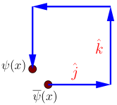
Here j,k=±1,±2,±3;jkformulae-sequence𝑗𝑘plus-or-minus1plus-or-minus2plus-or-minus3𝑗𝑘j,k=\pm 1,\pm 2,\pm 3;j\neq k and a𝑎a and b𝑏b are spinor indices for a total of 24×16=384241638424\times 16=384 operators. The j^^𝑗\hat{j} denotes a four-vector of unit length along the spatial axis j𝑗j. See Figure 1 for a diagrammatic representation of the building block operator.
Refer to caption
Figure 1: Diagrammatic representation of the building block operator.

Superpositions of such operators for meson spectrum analysis have been suggested and used previously in special cases Mandula (1984); Jorysz and Michael (1988); Lacock et al. (1996); Bernard et al. (1997). Evaluation of correlators constructed from operators of this form requires only calculation of propagators from a single source. Construction of operators transforming as irrep ΛPCsuperscriptΛ𝑃𝐶\Lambda^{PC} is facilitated by observing that one can effectively consider the transformation of the spinor and link paths independently and then combine them via octahedral Clebsch-Gordan coefficients. Link smearing can be performed on operators at both the source and sink of the correlator, and quark smearing at one end to suppress high energy states with no change to the symmetry of the symmetrized operators.

II.3 Spinor contribution to group structure

The contribution to the group structure due to spinor indices is determined by the 161616 bilinears ψ¯Fψ¯𝜓𝐹𝜓\overline{\psi}F\psi, where F𝐹F represents one of sixteen 4×4444\times 4 matrices, {I,γ5,γ4,γ4γ5,γi,γiγ5,σ4i,ϵijkσjk}𝐼subscript𝛾5subscript𝛾4subscript𝛾4subscript𝛾5subscript𝛾𝑖subscript𝛾𝑖subscript𝛾5subscript𝜎4𝑖subscriptitalic-ϵ𝑖𝑗𝑘subscript𝜎𝑗𝑘\{I,\gamma_{5},\gamma_{4},\gamma_{4}\gamma_{5},\gamma_{i},\gamma_{i}\gamma_{5},\sigma_{4i},\epsilon_{ijk}\sigma_{jk}\}. The first four bilinears are scalars while the last four three-index objects are vectors under the rotation group in the Euclidean continuum.

Parity (P𝑃P) and charge conjugation (C𝐶C) of the bilinears are identified via

𝒞ψ𝒞=(ψ¯C)T,𝒫ψ𝒫=γ4ψ,𝒞ψ¯𝒞=(Cψ)T,𝒫ψ¯𝒫=ψ¯γ4,𝒞𝜓superscript𝒞superscript¯𝜓superscript𝐶𝑇missing-subexpression𝒫𝜓superscript𝒫subscript𝛾4𝜓𝒞¯𝜓superscript𝒞superscript𝐶𝜓𝑇missing-subexpression𝒫¯𝜓superscript𝒫¯𝜓subscript𝛾4\begin{array}[]{ccc}\mathcal{C}\psi\mathcal{C}^{\dagger}=\left(\overline{\psi}C^{\dagger}\right)^{T},&&\mathcal{P}\psi\mathcal{P}^{\dagger}=\gamma_{4}\psi,\\ \mathcal{C}\overline{\psi}\mathcal{C}^{\dagger}=-\left(C\psi\right)^{T},&&\mathcal{P}\overline{\psi}\mathcal{P}^{\dagger}=\overline{\psi}\gamma_{4},\end{array} (5)

where C𝐶C is the matrix implementing charge conjugation and we have suppressed the action on coordinates, which under parity sees x=(x1,x2,x3,x4)xP𝑥subscript𝑥1subscript𝑥2subscript𝑥3subscript𝑥4subscript𝑥𝑃x=(x_{1},x_{2},x_{3},x_{4})\to x_{P}, where

xP=(x1,x2,x3,x4).subscript𝑥𝑃subscript𝑥1subscript𝑥2subscript𝑥3subscript𝑥4x_{P}=(-x_{1},-x_{2},-x_{3},x_{4}). (6)

To classify the bilinears into irreps of O𝑂O one uses its character table found in Table 3 to project out the octahedral irreps from the representations generated by the bilinears. Since the bilinears are scalars and vectors in the continuum it follows that their respective spans are also invariant under O𝑂O. By inspection it is straightforward to show that the character table for the scalar and vector bilinears is identical with that of A1subscript𝐴1A_{1} and T1subscript𝑇1T_{1} respectively. Since the multiplicity nΛJsubscriptsuperscript𝑛𝐽Λn^{J}_{\Lambda} of irrep ΛΛ\Lambda in any representation J𝐽J is given by Equation (2), it follows trivially that the scalar and vector bilinears form the basis of A1subscript𝐴1A_{1} and T1subscript𝑇1T_{1} irreps respectively.

Furthermore it may be verified that the ithsuperscript𝑖𝑡i^{th} vector bilinear component transforms as the ithsuperscript𝑖𝑡i^{th} row for our choice of matrix representation Γ(T1)(R)superscriptΓsubscript𝑇1𝑅\Gamma^{({T_{1}})}({R}) given in Table 4. Since the action on the spinor under rotation R𝑅R is ψ¯ψ¯S(R)¯𝜓¯𝜓𝑆𝑅\overline{\psi}\rightarrow\overline{\psi}S(R) and ψS(R)ψ𝜓superscript𝑆𝑅𝜓\psi\rightarrow S^{\dagger}(R)\psi, this amounts to verifying that

S(R)FiS(R)=jΓji(T1)(R)Fj,𝑆𝑅subscript𝐹𝑖superscript𝑆𝑅subscript𝑗subscriptsuperscriptΓsubscript𝑇1𝑗𝑖𝑅subscript𝐹𝑗S(R)F_{i}S^{\dagger}(R)=\sum_{j}\Gamma^{({T_{1}})}_{{j}{i}}({R})F_{j}\;, (7)

for the elements R𝑅R of O𝑂O and the four different vector bilinears F𝐹F. Here S(R)𝑆𝑅S(R) is the matrix implementing the rotation on the spinors. It is sufficient to verify Equation (7) for the two generators, namely the π/2𝜋2\pi/2 rotations about the y𝑦y and z𝑧z axes, C4ysubscript𝐶4𝑦C_{4y} and C4zsubscript𝐶4𝑧C_{4z}, for which these matrices are given by

S(C4y)𝑆subscript𝐶4𝑦\displaystyle S(C_{4y}) =\displaystyle= 12(1+γ1γ3),121subscript𝛾1subscript𝛾3\displaystyle\frac{1}{\sqrt{2}}(1+\gamma_{1}\gamma_{3})\;, (8)
S(C4z)𝑆subscript𝐶4𝑧\displaystyle S(C_{4z}) =\displaystyle= 12(1+γ2γ1).121subscript𝛾2subscript𝛾1\displaystyle\frac{1}{\sqrt{2}}(1+\gamma_{2}\gamma_{1})\;. (9)
Table 4: Matrices ΓΓ\Gamma for the generators C4ysubscript𝐶4𝑦C_{4y} and C4zsubscript𝐶4𝑧C_{4z} of the octahedral group for each irrep ΛΛ\Lambda.
ΛΛ\Lambda Γ(Λ)(C4y)superscriptΓΛsubscript𝐶4𝑦\Gamma^{({\Lambda})}({C_{4y}}) Γ(Λ)(C4z)superscriptΓΛsubscript𝐶4𝑧\Gamma^{({\Lambda})}({C_{4z}})
A1subscript𝐴1A_{1} [1]delimited-[]1\left[\begin{array}[]{c}1\end{array}\right] [1]delimited-[]1\left[\begin{array}[]{c}1\end{array}\right]
A2subscript𝐴2A_{2} [1]delimited-[]1\left[\begin{array}[]{c}-1\end{array}\right] [1]delimited-[]1\left[\begin{array}[]{c}-1\end{array}\right]
E𝐸E 12[1331]12delimited-[]1331\frac{1}{2}\left[\begin{array}[]{cc}1&\sqrt{3}\\ \sqrt{3}&-1\end{array}\right] [1001]delimited-[]1001\left[\begin{array}[]{cc}-1&0\\ 0&1\end{array}\right]
T1subscript𝑇1T_{1} [001010100]delimited-[]001010100\left[\begin{array}[]{ccc}0&0&1\\ 0&1&0\\ -1&0&0\end{array}\right] [010100001]delimited-[]010100001\left[\begin{array}[]{ccc}0&-1&0\\ 1&0&0\\ 0&0&1\end{array}\right]
T2subscript𝑇2T_{2} [010100001]delimited-[]010100001\left[\begin{array}[]{ccc}0&1&0\\ -1&0&0\\ 0&0&-1\end{array}\right] [100001010]delimited-[]100001010\left[\begin{array}[]{ccc}-1&0&0\\ 0&0&1\\ 0&-1&0\end{array}\right]

Hence the reduction of the spinor structure of our operators is given in Table 5, where now each bilinear may be classified uniquely by its irrep ΛPCsuperscriptΛ𝑃𝐶\Lambda^{PC}, row λ𝜆\lambda, and irrep multiplicity index α𝛼\alpha as FλΛαPCsubscriptsuperscript𝐹superscriptΛ𝛼𝑃𝐶𝜆F^{\Lambda^{{\alpha}PC}}_{\lambda}.

Table 5: Octahedral symmetries of the spinor bilinears. The operators have been separated into quadrants according to their dependency on twist angle as discussed in Ref. Harnett et al. (2006).

FΛPCλαFΛPCλαIA1++11γiT1i1γ5A1+11γiγ5T1++i1γ4A1+11σ4iT1i2γ4γ5A1+12ϵijkσjkT1+i1missing-subexpressionmissing-subexpressionmissing-subexpressionmissing-subexpressionmissing-subexpressionmissing-subexpressionmissing-subexpressionmissing-subexpression𝐹superscriptΛ𝑃𝐶𝜆𝛼𝐹superscriptΛ𝑃𝐶𝜆𝛼missing-subexpressionmissing-subexpressionmissing-subexpressionmissing-subexpressionmissing-subexpressionmissing-subexpressionmissing-subexpressionmissing-subexpressionmissing-subexpressionmissing-subexpressionmissing-subexpressionmissing-subexpressionmissing-subexpressionmissing-subexpressionmissing-subexpressionmissing-subexpression𝐼superscriptsubscript𝐴1absent11subscript𝛾𝑖superscriptsubscript𝑇1absent𝑖1subscript𝛾5superscriptsubscript𝐴1absent11subscript𝛾𝑖subscript𝛾5superscriptsubscript𝑇1absent𝑖1missing-subexpressionmissing-subexpressionmissing-subexpressionmissing-subexpressionmissing-subexpressionmissing-subexpressionmissing-subexpressionmissing-subexpressionsubscript𝛾4superscriptsubscript𝐴1absent11subscript𝜎4𝑖superscriptsubscript𝑇1absent𝑖2subscript𝛾4subscript𝛾5superscriptsubscript𝐴1absent12subscriptitalic-ϵ𝑖𝑗𝑘subscript𝜎𝑗𝑘superscriptsubscript𝑇1absent𝑖1\begin{array}[]{|c|c|c|c||c|c|c|c|}\hline\cr F&\rule{0.0pt}{10.76385pt}\Lambda^{PC}&\lambda&{\alpha}&F&\rule{0.0pt}{10.76385pt}\Lambda^{PC}&\lambda&{\alpha}\\ \hline\cr\hline\cr{I}&\rule{0.0pt}{10.76385pt}{A_{1}^{++}}&{1}&{1}&{\gamma_{i}}&\rule{0.0pt}{10.76385pt}{T_{1}^{--}}&{i}&{1}\\ {\gamma_{5}}&\rule{0.0pt}{10.76385pt}{A_{1}^{-+}}&{1}&{1}&{\gamma_{i}\gamma_{5}}&\rule{0.0pt}{10.76385pt}{T_{1}^{++}}&{i}&{1}\\ \hline\cr{\gamma_{4}}&\rule{0.0pt}{10.76385pt}{A_{1}^{+-}}&{1}&{1}&{\sigma_{4i}}&\rule{0.0pt}{10.76385pt}{T_{1}^{--}}&{i}&{2}\\ {\gamma_{4}\gamma_{5}}&\rule{0.0pt}{10.76385pt}{A_{1}^{-+}}&{1}&{2}&{\epsilon_{ijk}\sigma_{jk}}&\rule{0.0pt}{10.76385pt}{T_{1}^{+-}}&{i}&{1}\\ \hline\cr\end{array}

II.4 Link contribution to group structure

As with the spinors, one can simplify the discussion of the rotational properties of the gauge links by considering first the parity and charge conjugation and only then the rotations in O𝑂O. Parity of a link about the point x𝑥x is implemented via inversion about all three spatial axes as usual. Charge conjugation sees UU𝑈superscript𝑈U\rightarrow U^{*}, however to compensate for an overall transpose arising from the transformation of our quark bilinear, we formally transform UU𝑈superscript𝑈U\rightarrow U^{\dagger} to achieve the correct overall charge conjugation properties of our operators. The parity and charge conjugation contributions due to this link structure can then be taken into account by defining the PC𝑃𝐶PC-adapted superpositions,

Ui,jPC=12(Uj,k+PUj,k+CUk,j+PCUk,j),subscriptsuperscript𝑈𝑃𝐶𝑖𝑗12subscript𝑈𝑗𝑘𝑃subscript𝑈𝑗𝑘𝐶subscript𝑈𝑘𝑗𝑃𝐶subscript𝑈𝑘𝑗U^{PC}_{i,j}=\frac{1}{2}\left(U_{j,k}+PU_{-j,-k}+CU_{k,j}+PCU_{-k,-j}\right)\;, (10)

where k𝑘k is defined via k^=i^×j^^𝑘^𝑖^𝑗\hat{k}=\hat{i}\times\hat{j}. Diagrammatically, Ui,jPCsubscriptsuperscript𝑈𝑃𝐶𝑖𝑗U^{PC}_{i,j} is shown in Figure 2.

Refer to caption
Figure 2: PC𝑃𝐶PC-symmetrized basis elements for gauge field links. We have suppressed the overall normalization factor of 1/2121/2.

For fixed P𝑃P and C𝐶C the space spanned by Ui,jPCsubscriptsuperscript𝑈𝑃𝐶𝑖𝑗U^{PC}_{i,j} is invariant under O𝑂O and will generate a representation UPCsuperscript𝑈𝑃𝐶U^{PC} of the group. A basis for the six-dimensional space may be found by restricting (i,j)𝑖𝑗(i,j) to {(1,2),(1,3),(2,3),(2,1),(3,1),(3,2)}121323213132\{(1,2),(1,3),(2,3),(2,1),(3,1),(3,2)\} and this will in turn induce the particular matrix representation Γ(i,j)(m,n)(UPC)(R)subscriptsuperscriptΓsuperscript𝑈𝑃𝐶𝑖𝑗𝑚𝑛𝑅\Gamma^{({U^{PC}})}_{{(i,j)}{(m,n)}}({R}).

In order to determine how each of these four six-dimensional representations reduces, it is convenient to calculate their respective character tables. A straightforward consideration of the effect of a single element from each class of O𝑂O on the basis vectors allows one to find the character table for UPCsuperscript𝑈𝑃𝐶U^{PC} shown in Table 6.

Table 6: Character table showing χ(UPC)(ξ)superscript𝜒superscript𝑈𝑃𝐶𝜉\chi^{(U^{PC})}(\xi) for representation UPCsuperscript𝑈𝑃𝐶U^{PC} induced by Ui,jPCsubscriptsuperscript𝑈𝑃𝐶𝑖𝑗U^{PC}_{i,j}. Here positive and negative are to be interpreted as +11+1 and 11-1 in the entries.

E3C428C36C46C262P00(P+1)Cmissing-subexpressionmissing-subexpressionmissing-subexpressionmissing-subexpressionmissing-subexpression𝐸3superscriptsubscript𝐶428subscript𝐶36subscript𝐶46subscript𝐶2missing-subexpressionmissing-subexpressionmissing-subexpressionmissing-subexpressionmissing-subexpression62𝑃00𝑃1𝐶\begin{array}[]{|ccccc|}\hline\cr E&3C_{4}^{2}&8C_{3}&6C_{4}&6C_{2}\\ \hline\cr 6&2P&0&0&(P+1)C\\ \hline\cr\end{array}

Use of Equation (2) with J𝐽J as UPCsuperscript𝑈𝑃𝐶U^{PC} reduces the latter to irreps ΛPCsuperscriptΛ𝑃𝐶\Lambda^{PC} of OPCsuperscript𝑂𝑃𝐶O^{PC} as shown in Table 7. So, for example, U++=A1++E++T2++superscript𝑈absentdirect-sumsuperscriptsubscript𝐴1absentsuperscript𝐸absentsuperscriptsubscript𝑇2absentU^{++}=A_{1}^{++}\oplus E^{++}\oplus T_{2}^{++}.

Table 7: Reduction of UPCsuperscript𝑈𝑃𝐶U^{PC} to irreps ΛPCsuperscriptΛ𝑃𝐶\Lambda^{PC} of OPCsuperscript𝑂𝑃𝐶O^{PC}.

PCA1PCA2PCEPCT1PCT2PC++10101+01110+0001100011missing-subexpressionmissing-subexpressionmissing-subexpressionmissing-subexpressionmissing-subexpressionmissing-subexpressionmissing-subexpression𝑃𝐶superscriptsubscript𝐴1𝑃𝐶superscriptsubscript𝐴2𝑃𝐶superscript𝐸𝑃𝐶superscriptsubscript𝑇1𝑃𝐶superscriptsubscript𝑇2𝑃𝐶missing-subexpressionmissing-subexpressionmissing-subexpressionmissing-subexpressionmissing-subexpressionmissing-subexpressionmissing-subexpression10101011100001100011\begin{array}[]{|cc|ccccc|}\hline\cr P&C&\rule{0.0pt}{10.76385pt}A_{1}^{PC}&A_{2}^{PC}&E^{PC}&T_{1}^{PC}&T_{2}^{PC}\\ \hline\cr+&+&1&0&1&0&1\\ +&-&0&1&1&1&0\\ -&+&0&0&0&1&1\\ -&-&0&0&0&1&1\\ \hline\cr\end{array}

To arrive at the explicit form of the lattice-symmetrized gauge links, note that, by Table 7, each of our spaces reduces to no more than a single copy of each irrep. For such simply reducible representations the reduction is straightforward333See Ref. (Cornwell, 1997, page 74) where the Clebsch-Gordan coefficients for a simply reducible direct product representation are given. In the case at hand one simply considers an arbitrary representation in place of the direct product to arrive at our result. and in our case one has the following formula for the symmetrized link fields:

UλΛPC(x)=subscriptsuperscript𝑈superscriptΛ𝑃𝐶𝜆𝑥absent\displaystyle U^{\Lambda^{PC}}_{\lambda}(x)=
(i,j)ROΓ(i,j)(m,n)(UPC)(R)Γλμ(Λ)(R)[gOdΛROΓ(m,n)(m,n)(UPC)(R)Γμμ(Λ)(R)]12Ui,jPC(x),subscript𝑖𝑗subscript𝑅𝑂subscriptsuperscriptΓsuperscript𝑈𝑃𝐶𝑖𝑗𝑚𝑛𝑅subscriptsuperscriptΓΛ𝜆𝜇superscript𝑅superscriptdelimited-[]subscript𝑔𝑂subscript𝑑Λsubscript𝑅𝑂subscriptsuperscriptΓsuperscript𝑈𝑃𝐶𝑚𝑛𝑚𝑛𝑅subscriptsuperscriptΓΛ𝜇𝜇superscript𝑅12subscriptsuperscript𝑈𝑃𝐶𝑖𝑗𝑥\displaystyle\sum_{(i,j)}\frac{\sum_{R\in O}\Gamma^{({U^{PC}})}_{{(i,j)}{(m,n)}}({R})\Gamma^{({\Lambda})}_{{\lambda}{\mu}}({R})^{*}}{\left[\frac{g_{\scriptscriptstyle{{O}}}}{d_{\Lambda}}\sum_{R\in O}\Gamma^{({U^{PC}})}_{{(m,n)}{(m,n)}}({R})\Gamma^{({\Lambda})}_{{\mu}{\mu}}({R})^{*}\right]^{\frac{1}{2}}}U^{PC}_{i,j}(x)\ ,

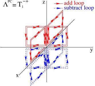
where (m,n)𝑚𝑛(m,n) and μ𝜇\mu are chosen so the denominator does not vanish and the accessible ΛPCsuperscriptΛ𝑃𝐶\Lambda^{PC} are taken from Table 7. Here Γλμ(Λ)(R)subscriptsuperscriptΓΛ𝜆𝜇𝑅\Gamma^{({\Lambda})}_{{\lambda}{\mu}}({R}) is the matrix representation for the irrep ΛΛ\Lambda of dimension dΛsubscript𝑑Λd_{\Lambda} taken from Table 4. Lowercase Greek denotes row indices of the group O𝑂O, and the sum is taken over the six pairs (i,j)𝑖𝑗(i,j) listed above. The UλΛPC(x)subscriptsuperscript𝑈superscriptΛ𝑃𝐶𝜆𝑥U^{\Lambda^{PC}}_{\lambda}(x) transform as the row λ𝜆\lambda of irrep ΛPCsuperscriptΛ𝑃𝐶\Lambda^{PC} and may be uniquely identified by these latter parameters. (Since each ΛPCsuperscriptΛ𝑃𝐶\Lambda^{PC} occurs only once in Table 7 there is no need, unlike in the spinor case, to further identify a multiplicity for the irrep.) Using the explicit irrep generator matrices in Table 4 to construct the full matrix representations for each irrep, one can evaluate Equation (II.4) to produce the final lattice-symmetrized gauge links. The results are tabulated in Table 8. A diagram of a lattice-symmetrized gauge link structure is shown in Figure 3.

In Equation (10), all the link structures with PC++PC\neq++ are suppressed by powers of lattice spacing relative to PC=++PC=++. Further factors of lattice spacing can appear when Equation (10) is used to form a gauge structure like the one shown in Figure 3. Such overall factors of lattice spacing will not be of direct relevance to our study of the mass spectrum, but would be of greater interest for decay constants and matrix elements.
Refer to caption
Figure 3: Extended gauge structure UλΛPC=U3T1+subscriptsuperscript𝑈superscriptΛ𝑃𝐶𝜆subscriptsuperscript𝑈superscriptsubscript𝑇1absent3U^{\Lambda^{PC}}_{\lambda}=U^{T_{1}^{-+}}_{3} is shown. Parity and charge conjugation symmetries are readily verified. The T1subscript𝑇1T_{1} irrep has three rows, this being the λ=3𝜆3\lambda=3 component which is symmetric about the z𝑧z-axis. Illustrations of other lattice-symmetrized gauge structures may be found in Ref. von Hippel et al. (2007).
Table 8: Shown are the lattice-symmetrized gauge links, UλΛPC(x)subscriptsuperscript𝑈superscriptΛ𝑃𝐶𝜆𝑥U^{\Lambda^{PC}}_{\lambda}(x), derived from Equation (II.4) in terms of the PC𝑃𝐶PC-adapted gauge field structures Ui,jPC(x)subscriptsuperscript𝑈𝑃𝐶𝑖𝑗𝑥U^{PC}_{i,j}(x). Each subtable corresponds to a different PC𝑃𝐶PC combination and contains the lattice-symmetrized gauge link combinations along the top, denoted by ΛλsuperscriptΛ𝜆\Lambda^{\lambda}, and the PC𝑃𝐶PC-adapted structures along the left, denoted by U(i,j)𝑈𝑖𝑗U(i,j). For irreps of dimension one the superscript denoting the row λ𝜆\lambda of the lattice-symmetrized link structure is suppressed. The actual coefficient equals the sign of the entry times the square root of the absolute value of the entry in the table. Thus, for example, one has U3T1+=(U1,2++U1,3++U2,3+U2,1+)/2subscriptsuperscript𝑈superscriptsubscript𝑇1absent3subscriptsuperscript𝑈absent12subscriptsuperscript𝑈absent13subscriptsuperscript𝑈absent23subscriptsuperscript𝑈absent212U^{T_{1}^{-+}}_{3}=\left(U^{-+}_{1,2}+U^{-+}_{1,3}+U^{-+}_{2,3}-U^{-+}_{2,1}\right)/2, which in turn can be expanded via Equation (10) to arrive at Figure 3.
PC=++A1E1E2T21T22T23U(1,2) 1/6 1/41/12 0 1/2 0U(1,3) 1/6 1/41/12 01/2 0U(2,3) 1/61/41/12 0 0 1/2U(2,1) 1/61/41/12 0 01/2U(3,1) 1/6 0 1/3 1/2 0 0U(3,2) 1/6 0 1/31/2 0 0\begin{array}[]{|c|rrrrrr|}\hline\cr\hline\cr PC=++&A_{1}&E^{1}&E^{2}&T_{2}^{1}&T_{2}^{2}&T_{2}^{3}\\ \hline\cr U(1,2)&\ 1/6&\ 1/4&-1/12&\ \ \ 0&\ 1/2&\ \ \ 0\\ U(1,3)&\ 1/6&\ 1/4&-1/12&\ \ \ 0&-1/2&\ \ \ 0\\ U(2,3)&\ 1/6&-1/4&-1/12&\ \ \ 0&\ \ \ 0&\ 1/2\\ U(2,1)&\ 1/6&-1/4&-1/12&\ \ \ 0&\ \ \ 0&-1/2\\ U(3,1)&\ 1/6&\ \ \ 0&\ 1/3&\ 1/2&\ \ \ 0&\ \ \ 0\\ U(3,2)&\ 1/6&\ \ \ 0&\ 1/3&-1/2&\ \ \ 0&\ \ \ 0\\ \hline\cr\hline\cr\end{array} PC=+A2E1E2T11T12T13U(1,2) 1/61/12 1/4  1/2 0 0U(1,3)1/61/121/4  1/2 0 0U(2,3) 1/61/121/4 0  1/2 0U(2,1)1/61/12 1/4 0  1/2 0U(3,1) 1/61/3 0 0 0  1/2U(3,2)1/6 1/3 0 0 0  1/2\begin{array}[]{|c|rrrrrr|}\hline\cr\hline\cr PC=+-&A_{2}&E^{1}&E^{2}&T_{1}^{1}&T_{1}^{2}&T_{1}^{3}\\ \hline\cr U(1,2)&\ 1/6&1/12&\ 1/4&\ \;1/2&\ \ \ 0&\ \ \ 0\\ U(1,3)&-1/6&-1/12&-1/4&\ \;1/2&\ \ \ 0&\ \ \ 0\\ U(2,3)&\ 1/6&1/12&-1/4&\ \ \ 0&\ \;1/2&\ \ \ 0\\ U(2,1)&-1/6&-1/12&\ 1/4&\ \ \ 0&\ \;1/2&\ \ \ 0\\ U(3,1)&\ 1/6&-1/3&\ \ \ 0&\ \ \ 0&\ \ \ 0&\ \;1/2\\ U(3,2)&-1/6&\ 1/3&\ \ \ 0&\ \ \ 0&\ \ \ 0&\ \;1/2\\ \hline\cr\hline\cr\end{array}
PC=+T11T12T13T21T22T23U(1,2) 0 1/4 1/4 1/4 01/4U(1,3) 01/4 1/4 1/4 0 1/4U(2,3) 1/4 0 1/41/4 1/4 0U(2,1) 1/4 01/4 1/4 1/4 0U(3,1) 1/4 1/4 0 01/4 1/4U(3,2)1/4 1/4 0 0 1/4 1/4\begin{array}[]{|c|rrrrrr|}\hline\cr\hline\cr PC=-+&T_{1}^{1}&T_{1}^{2}&T_{1}^{3}&T_{2}^{1}&T_{2}^{2}&T_{2}^{3}\\ \hline\cr U(1,2)&\ \ \ 0&\ 1/4&\ 1/4&\ 1/4&\ \ \ 0&-1/4\\ U(1,3)&\ \ \ 0&-1/4&\ 1/4&\ 1/4&\ \ \ 0&\ 1/4\\ U(2,3)&\ 1/4&\ \ \ 0&\ 1/4&-1/4&\ 1/4&\ \ \ 0\\ U(2,1)&\ 1/4&\ \ \ 0&-1/4&\ 1/4&\ 1/4&\ \ \ 0\\ U(3,1)&\ 1/4&\ 1/4&\ \ \ 0&\ \ \ 0&-1/4&\ 1/4\\ U(3,2)&-1/4&\ 1/4&\ \ \ 0&\ \ \ 0&\ 1/4&\ 1/4\\ \hline\cr\hline\cr\end{array} PC=T11T12T13T21T22T23U(1,2) 01/4 1/4 1/4 0 1/4U(1,3) 01/41/41/4 0 1/4U(2,3) 1/4 01/4 1/4 1/4 0U(2,1)1/4 01/4 1/41/4 0U(3,1)1/4 1/4 0 0 1/4 1/4U(3,2)1/41/4 0 0 1/41/4\begin{array}[]{|c|rrrrrr|}\hline\cr\hline\cr PC=--&T_{1}^{1}&T_{1}^{2}&T_{1}^{3}&T_{2}^{1}&T_{2}^{2}&T_{2}^{3}\\ \hline\cr U(1,2)&\ \ \ 0&-1/4&\ 1/4&\ 1/4&\ \ \ 0&\ 1/4\\ U(1,3)&\ \ \ 0&-1/4&-1/4&-1/4&\ \ \ 0&\ 1/4\\ U(2,3)&\ 1/4&\ \ \ 0&-1/4&\ 1/4&\ 1/4&\ \ \ 0\\ U(2,1)&-1/4&\ \ \ 0&-1/4&\ 1/4&-1/4&\ \ \ 0\\ U(3,1)&-1/4&\ 1/4&\ \ \ 0&\ \ \ 0&\ 1/4&\ 1/4\\ U(3,2)&-1/4&-1/4&\ \ \ 0&\ \ \ 0&\ 1/4&-1/4\\ \hline\cr\hline\cr\end{array}

II.5 Total representation reduction and operator construction

Having classified the spinor and link components of our operators into irreps of OPCsuperscript𝑂𝑃𝐶O^{PC}, it remains to combine them and reduce all possible direct product representations. Parity and charge conjugation for the product representations are given by

P=PfPuC=CfCu,𝑃subscript𝑃𝑓subscript𝑃𝑢missing-subexpression𝐶subscript𝐶𝑓subscript𝐶𝑢\begin{array}[]{ccc}P=P_{f}P_{u}&&C=C_{f}C_{u}\ ,\end{array} (12)

where f𝑓f corresponds to the fermionic part and u𝑢u corresponds to the gauge part. Noting that the character of a direct product representation like ΛfΛutensor-productsubscriptΛ𝑓subscriptΛ𝑢\Lambda_{f}\otimes\Lambda_{u} satisfies χ(ΛfΛu)(ξ)=χ(Λf)(ξ)χ(Λu)(ξ)superscript𝜒tensor-productsubscriptΛ𝑓subscriptΛ𝑢𝜉superscript𝜒subscriptΛ𝑓𝜉superscript𝜒subscriptΛ𝑢𝜉\chi^{(\Lambda_{f}\otimes\Lambda_{u})}(\xi)=\chi^{(\Lambda_{f})}(\xi)\chi^{(\Lambda_{u})}(\xi) and using Equation (2) with J=ΛfΛu𝐽tensor-productsubscriptΛ𝑓subscriptΛ𝑢J=\Lambda_{f}\otimes\Lambda_{u} and the characters in Table 3, one may reduce the octahedral part of each direct product into irreps of O𝑂O as shown in Table 9.

Table 9: Reduction of product representations ΛfΛutensor-productsubscriptΛ𝑓subscriptΛ𝑢\Lambda_{f}\otimes\Lambda_{u} into irreps of O𝑂O. Only irreps A1subscript𝐴1A_{1} and T1subscript𝑇1T_{1} are accessible for ΛfsubscriptΛ𝑓\Lambda_{f}. Reduction of other octahedral direct products may be inferred from Table 11.

A1A2ET1T2A1A1A2ET1T2T1T1T2T1T2A1ET1T2A2ET1T2missing-subexpressionmissing-subexpressionmissing-subexpressionmissing-subexpressionmissing-subexpressionmissing-subexpressiontensor-productsubscript𝐴1subscript𝐴2𝐸subscript𝑇1subscript𝑇2missing-subexpressionmissing-subexpressionmissing-subexpressionmissing-subexpressionmissing-subexpressionmissing-subexpressionsubscript𝐴1subscript𝐴1subscript𝐴2𝐸subscript𝑇1subscript𝑇2subscript𝑇1subscript𝑇1subscript𝑇2direct-sumsubscript𝑇1subscript𝑇2direct-sumsubscript𝐴1𝐸subscript𝑇1subscript𝑇2direct-sumsubscript𝐴2𝐸subscript𝑇1subscript𝑇2\begin{array}[]{|c|ccccc|}\hline\cr\otimes&A_{1}&A_{2}&E&T_{1}&T_{2}\\ \hline\cr A_{1}&A_{1}&A_{2}&E&T_{1}&T_{2}\\ T_{1}&T_{1}&T_{2}&T_{1}\oplus T_{2}&A_{1}\oplus E\oplus T_{1}\oplus T_{2}&A_{2}\oplus E\oplus T_{1}\oplus T_{2}\\ \hline\cr\end{array}

The results shown in Tables 5, 7, and 9 along with Equation (12) finally allow the 384384384-dimensional representation generated by the space spanned by Mj,k,a,b(t)subscript𝑀𝑗𝑘𝑎𝑏𝑡M_{j,k,a,b}(t) to be reduced into irreps of OPCsuperscript𝑂𝑃𝐶O^{PC} as shown in Table 10. It is of note that while the local quark operators can access only irreps of the form A1PCsuperscriptsubscript𝐴1𝑃𝐶A_{1}^{PC} and T1PCsuperscriptsubscript𝑇1𝑃𝐶T_{1}^{PC} of OPCsuperscript𝑂𝑃𝐶O^{PC}, the addition of extended gauge field structure admits operators of every possible irrep. In principle, then, this set of operators can couple to all meson states.

Table 10: Reduction of the representation generated by the span of Mj,k,a,b(t)subscript𝑀𝑗𝑘𝑎𝑏𝑡M_{j,k,a,b}(t) into OPCsuperscript𝑂𝑃𝐶O^{PC} irreps. The 384-dimensional representation reduces into the sum of the irreps listed in this table with multiplicities shown.

Λ\PC++++A14462A24426E8888T112121014T212121410missing-subexpressionmissing-subexpressionmissing-subexpressionmissing-subexpressionmissing-subexpression\Λ𝑃𝐶missing-subexpressionmissing-subexpressionmissing-subexpressionmissing-subexpressionmissing-subexpressionsubscript𝐴14462subscript𝐴24426𝐸8888subscript𝑇112121014subscript𝑇212121410\begin{array}[]{|c|rrrr|}\hline\cr\Lambda\backslash PC&++&+-&-+&--\\ \hline\cr A_{1}&4&4&6&2\\ A_{2}&4&4&2&6\\ E&8&8&8&8\\ T_{1}&12&12&10&14\\ T_{2}&12&12&14&10\\ \hline\cr\end{array}

The construction of the lattice-symmetrized operators themselves is accomplished by combining the spinor and link operator components FλΛαPCsubscriptsuperscript𝐹superscriptΛ𝛼𝑃𝐶𝜆F^{\Lambda^{{\alpha}PC}}_{\lambda} and UλΛPCsubscriptsuperscript𝑈superscriptΛ𝑃𝐶𝜆U^{\Lambda^{PC}}_{\lambda} using the same formulae for parity and charge conjugation given in Equation (12) and by combining the irreps of O𝑂O using Clebsch-Gordan (C-G) coefficients for the reduction of a direct product of two irreps of O𝑂O, Λ1Λ2tensor-productsubscriptΛ1subscriptΛ2{\Lambda_{1}}\otimes{\Lambda_{2}}. As suggested by Table 9, the direct product representations for irreps of O𝑂O are simply reducible, allowing one to use the formula

(Λ1Λ2Λλ1λ2λ)=subscriptΛ1subscriptΛ2Λsubscript𝜆1subscript𝜆2𝜆absent\displaystyle\left(\begin{array}[]{cc|c}{\Lambda_{1}}&{\Lambda_{2}}&\Lambda\\ {\lambda_{1}}&{\lambda_{2}}&\lambda\end{array}\right)= (16)
ROΓλ1μ1(Λ1)(R)Γλ2μ2(Λ2)(R)Γλμ(Λ)(R)[gOdΛROΓμ1μ1(Λ1)(R)Γμ2μ2(Λ2)(R)Γμμ(Λ)(R)]12subscript𝑅𝑂subscriptsuperscriptΓsubscriptΛ1subscript𝜆1subscript𝜇1𝑅subscriptsuperscriptΓsubscriptΛ2subscript𝜆2subscript𝜇2𝑅subscriptsuperscriptΓΛ𝜆𝜇superscript𝑅superscriptdelimited-[]subscript𝑔𝑂subscript𝑑Λsubscript𝑅𝑂subscriptsuperscriptΓsubscriptΛ1subscript𝜇1subscript𝜇1𝑅subscriptsuperscriptΓsubscriptΛ2subscript𝜇2subscript𝜇2𝑅subscriptsuperscriptΓΛ𝜇𝜇superscript𝑅12\displaystyle\frac{\sum_{R\in O}\Gamma^{({{\Lambda_{1}}})}_{{{\lambda_{1}}}{{\mu_{1}}}}({R})\Gamma^{({{\Lambda_{2}}})}_{{{\lambda_{2}}}{{\mu_{2}}}}({R})\Gamma^{({\Lambda})}_{{\lambda}{\mu}}({R})^{*}}{\left[\frac{g_{\scriptscriptstyle{{O}}}}{d_{\Lambda}}\sum_{R\in O}\Gamma^{({{\Lambda_{1}}})}_{{{\mu_{1}}}{{\mu_{1}}}}({R})\Gamma^{({{\Lambda_{2}}})}_{{{\mu_{2}}}{{\mu_{2}}}}({R})\Gamma^{({\Lambda})}_{{\mu}{\mu}}({R})^{*}\right]^{\frac{1}{2}}}

to determine the C-G coefficients. (See Ref. (Cornwell, 1997, page 74).) Here μ𝜇\mu, μ1subscript𝜇1{\mu_{1}}, and μ2subscript𝜇2{\mu_{2}} are chosen so the denominator does not vanish. Using the irrep generators given in Table 4, these C-G coefficients have been calculated and are given in Table 11. The lattice-symmetrized operators, MλΛPC(t)subscriptsuperscript𝑀superscriptΛ𝑃𝐶𝜆𝑡M^{\Lambda^{PC}}_{\lambda}(t), are finally

MλΛPC,ΛfαfPfCf,ΛuPuCu(t)=superscriptsubscript𝑀𝜆superscriptΛ𝑃𝐶superscriptsubscriptΛ𝑓subscript𝛼𝑓subscript𝑃𝑓subscript𝐶𝑓superscriptsubscriptΛ𝑢subscript𝑃𝑢subscript𝐶𝑢𝑡absent\displaystyle M_{\lambda}^{\Lambda^{PC},\Lambda_{f}^{{\alpha}_{f}P_{f}C_{f}},\Lambda_{u}^{P_{u}C_{u}}}(t)= (20)
𝐱λf,λu(ΛfΛuΛλfλuλ)ψ¯(x)FλfΛfαfPfCfUλuΛuPuCu(x)ψ(x),subscript𝐱subscriptsubscript𝜆𝑓subscript𝜆𝑢subscriptΛ𝑓subscriptΛ𝑢Λsubscript𝜆𝑓subscript𝜆𝑢𝜆¯𝜓𝑥subscriptsuperscript𝐹superscriptsubscriptΛ𝑓subscript𝛼𝑓subscript𝑃𝑓subscript𝐶𝑓subscript𝜆𝑓subscriptsuperscript𝑈superscriptsubscriptΛ𝑢subscript𝑃𝑢subscript𝐶𝑢subscript𝜆𝑢𝑥𝜓𝑥\displaystyle{\displaystyle\sum_{\mathbf{{x}}}\sum_{\lambda_{f},\lambda_{u}}}\left(\begin{array}[]{cc|c}\Lambda_{f}&\Lambda_{u}&\Lambda\\ \lambda_{f}&\lambda_{u}&\lambda\end{array}\right)\overline{\psi}(x)F^{\Lambda_{f}^{{\alpha}_{f}P_{f}C_{f}}}_{\lambda_{f}}U^{\Lambda_{u}^{P_{u}C_{u}}}_{\lambda_{u}}(x)\psi(x)\;,

where the allowed irreps for the spinor bilinear and link components are determined by Tables 5 and 7. These fix P𝑃P and C𝐶C for the operator while the irreps ΛΛ\Lambda of O𝑂O are those allowed by the C-G series in Table 9. Dirac indices on F𝐹F and color indices on U𝑈U and both indices on the spinors have been suppressed. We note that each operator is thus uniquely identified by its irrep ΛΛ\Lambda, its row λ𝜆\lambda, and the direct product from which it originates, ΛfαfPfCfΛuPuCutensor-productsuperscriptsubscriptΛ𝑓subscript𝛼𝑓subscript𝑃𝑓subscript𝐶𝑓superscriptsubscriptΛ𝑢subscript𝑃𝑢subscript𝐶𝑢\Lambda_{f}^{{\alpha}_{f}P_{f}C_{f}}\otimes\Lambda_{u}^{P_{u}C_{u}}.

Table 11: Octahedral group Clebsch-Gordan coefficients derived from Equation (16). The actual coefficient equals the sign of the entry times the square root of its absolute value. Superscripts on irreps denote the row. If the irrep is one-dimensional the superscript is suppressed. Since the C-G coefficients for Λ1Λ2tensor-productsubscriptΛ1subscriptΛ2{\Lambda_{1}}\otimes{\Lambda_{2}} are the same as for Λ2Λ1tensor-productsubscriptΛ2subscriptΛ1{\Lambda_{2}}\otimes{\Lambda_{1}} only one combination is listed.
A1A1A1A1A1 1missing-subexpressionmissing-subexpressionmissing-subexpressionmissing-subexpressiontensor-productsubscript𝐴1subscript𝐴1subscript𝐴1missing-subexpressionmissing-subexpressionsubscript𝐴1subscript𝐴11missing-subexpressionmissing-subexpression\begin{array}[]{|c|r|}\hline\cr\hline\cr A_{1}\otimes A_{1}&A_{1}\\ \hline\cr A_{1}A_{1}&\ \ \ 1\\ \hline\cr\hline\cr\end{array}
A1A2A2A1A2 1missing-subexpressionmissing-subexpressionmissing-subexpressionmissing-subexpressiontensor-productsubscript𝐴1subscript𝐴2subscript𝐴2missing-subexpressionmissing-subexpressionsubscript𝐴1subscript𝐴21missing-subexpressionmissing-subexpression\begin{array}[]{|c|r|}\hline\cr\hline\cr A_{1}\otimes A_{2}&A_{2}\\ \hline\cr A_{1}A_{2}&\ \ \ 1\\ \hline\cr\hline\cr\end{array}
A2A2A1A2A2 1missing-subexpressionmissing-subexpressionmissing-subexpressionmissing-subexpressiontensor-productsubscript𝐴2subscript𝐴2subscript𝐴1missing-subexpressionmissing-subexpressionsubscript𝐴2subscript𝐴21missing-subexpressionmissing-subexpression\begin{array}[]{|c|r|}\hline\cr\hline\cr A_{2}\otimes A_{2}&A_{1}\\ \hline\cr A_{2}A_{2}&\ \ \ 1\\ \hline\cr\hline\cr\end{array}
A1EE1E2A1E1 1 0A1E2 0 1missing-subexpressionmissing-subexpressionmissing-subexpressionmissing-subexpressionmissing-subexpressionmissing-subexpressiontensor-productsubscript𝐴1𝐸superscript𝐸1superscript𝐸2missing-subexpressionmissing-subexpressionmissing-subexpressionsubscript𝐴1superscript𝐸11 0subscript𝐴1superscript𝐸2 01missing-subexpressionmissing-subexpressionmissing-subexpression\begin{array}[]{|c|rr|}\hline\cr\hline\cr A_{1}\otimes E&E^{1}&E^{2}\\ \hline\cr A_{1}E^{1}&\ \ \ 1&\ \ \ 0\\ A_{1}E^{2}&\ \ \ 0&\ \ \ 1\\ \hline\cr\hline\cr\end{array}
A2EE1E2A2E1 0 1A2E21 0missing-subexpressionmissing-subexpressionmissing-subexpressionmissing-subexpressionmissing-subexpressionmissing-subexpressiontensor-productsubscript𝐴2𝐸superscript𝐸1superscript𝐸2missing-subexpressionmissing-subexpressionmissing-subexpressionsubscript𝐴2superscript𝐸1 01subscript𝐴2superscript𝐸21 0missing-subexpressionmissing-subexpressionmissing-subexpression\begin{array}[]{|c|rr|}\hline\cr\hline\cr A_{2}\otimes E&E^{1}&E^{2}\\ \hline\cr A_{2}E^{1}&\ \ \ 0&\ \ \ 1\\ A_{2}E^{2}&\ \ -1&\ \ \ 0\\ \hline\cr\hline\cr\end{array}
A1T1T11T12T13A1T11 1 0 0A1T12 0 1 0A1T13 0 0 1missing-subexpressionmissing-subexpressionmissing-subexpressionmissing-subexpressionmissing-subexpressionmissing-subexpressionmissing-subexpressionmissing-subexpressiontensor-productsubscript𝐴1subscript𝑇1superscriptsubscript𝑇11superscriptsubscript𝑇12superscriptsubscript𝑇13missing-subexpressionmissing-subexpressionmissing-subexpressionmissing-subexpressionsubscript𝐴1superscriptsubscript𝑇111 0 0subscript𝐴1superscriptsubscript𝑇12 01 0subscript𝐴1superscriptsubscript𝑇13 0 01missing-subexpressionmissing-subexpressionmissing-subexpressionmissing-subexpression\begin{array}[]{|c|rrr|}\hline\cr\hline\cr A_{1}\otimes T_{1}&T_{1}^{1}&T_{1}^{2}&T_{1}^{3}\\ \hline\cr A_{1}T_{1}^{1}&\ \ \ 1&\ \ \ 0&\ \ \ 0\\ A_{1}T_{1}^{2}&\ \ \ 0&\ \ \ 1&\ \ \ 0\\ A_{1}T_{1}^{3}&\ \ \ 0&\ \ \ 0&\ \ \ 1\\ \hline\cr\hline\cr\end{array} A1T2T21T22T23A1T21 1 0 0A1T22 0 1 0A1T23 0 0 1missing-subexpressionmissing-subexpressionmissing-subexpressionmissing-subexpressionmissing-subexpressionmissing-subexpressionmissing-subexpressionmissing-subexpressiontensor-productsubscript𝐴1subscript𝑇2superscriptsubscript𝑇21superscriptsubscript𝑇22superscriptsubscript𝑇23missing-subexpressionmissing-subexpressionmissing-subexpressionmissing-subexpressionsubscript𝐴1superscriptsubscript𝑇211 0 0subscript𝐴1superscriptsubscript𝑇22 01 0subscript𝐴1superscriptsubscript𝑇23 0 01missing-subexpressionmissing-subexpressionmissing-subexpressionmissing-subexpression\begin{array}[]{|c|rrr|}\hline\cr\hline\cr A_{1}\otimes T_{2}&T_{2}^{1}&T_{2}^{2}&T_{2}^{3}\\ \hline\cr A_{1}T_{2}^{1}&\ \ \ 1&\ \ \ 0&\ \ \ 0\\ A_{1}T_{2}^{2}&\ \ \ 0&\ \ \ 1&\ \ \ 0\\ A_{1}T_{2}^{3}&\ \ \ 0&\ \ \ 0&\ \ \ 1\\ \hline\cr\hline\cr\end{array}
A2T1T21T22T23A2T11 0 1 0A2T12 0 0 1A2T13 1 0 0missing-subexpressionmissing-subexpressionmissing-subexpressionmissing-subexpressionmissing-subexpressionmissing-subexpressionmissing-subexpressionmissing-subexpressiontensor-productsubscript𝐴2subscript𝑇1superscriptsubscript𝑇21superscriptsubscript𝑇22superscriptsubscript𝑇23missing-subexpressionmissing-subexpressionmissing-subexpressionmissing-subexpressionsubscript𝐴2superscriptsubscript𝑇11 01 0subscript𝐴2superscriptsubscript𝑇12 0 01subscript𝐴2superscriptsubscript𝑇131 0 0missing-subexpressionmissing-subexpressionmissing-subexpressionmissing-subexpression\begin{array}[]{|c|rrr|}\hline\cr\hline\cr A_{2}\otimes T_{1}&T_{2}^{1}&T_{2}^{2}&T_{2}^{3}\\ \hline\cr A_{2}T_{1}^{1}&\ \ \ 0&\ \ \ 1&\ \ \ 0\\ A_{2}T_{1}^{2}&\ \ \ 0&\ \ \ 0&\ \ \ 1\\ A_{2}T_{1}^{3}&\ \ \ 1&\ \ \ 0&\ \ \ 0\\ \hline\cr\hline\cr\end{array} A2T2T11T12T13A2T21 0 0 1A2T22 1 0 0A2T23 0 1 0missing-subexpressionmissing-subexpressionmissing-subexpressionmissing-subexpressionmissing-subexpressionmissing-subexpressionmissing-subexpressionmissing-subexpressiontensor-productsubscript𝐴2subscript𝑇2superscriptsubscript𝑇11superscriptsubscript𝑇12superscriptsubscript𝑇13missing-subexpressionmissing-subexpressionmissing-subexpressionmissing-subexpressionsubscript𝐴2superscriptsubscript𝑇21 0 01subscript𝐴2superscriptsubscript𝑇221 0 0subscript𝐴2superscriptsubscript𝑇23 01 0missing-subexpressionmissing-subexpressionmissing-subexpressionmissing-subexpression\begin{array}[]{|c|rrr|}\hline\cr\hline\cr A_{2}\otimes T_{2}&T_{1}^{1}&T_{1}^{2}&T_{1}^{3}\\ \hline\cr A_{2}T_{2}^{1}&\ \ \ 0&\ \ \ 0&\ \ \ 1\\ A_{2}T_{2}^{2}&\ \ \ 1&\ \ \ 0&\ \ \ 0\\ A_{2}T_{2}^{3}&\ \ \ 0&\ \ \ 1&\ \ \ 0\\ \hline\cr\hline\cr\end{array}
EEA1A2E1E2E1E1 1/2 0 0 1/2E1E2 0 1/2 1/2 0E2E1 01/2 1/2 0E2E2 1/2 0 01/2missing-subexpressionmissing-subexpressionmissing-subexpressionmissing-subexpressionmissing-subexpressionmissing-subexpressionmissing-subexpressionmissing-subexpressionmissing-subexpressionmissing-subexpressiontensor-product𝐸𝐸subscript𝐴1subscript𝐴2superscript𝐸1superscript𝐸2missing-subexpressionmissing-subexpressionmissing-subexpressionmissing-subexpressionmissing-subexpressionsuperscript𝐸1superscript𝐸112 0 012superscript𝐸1superscript𝐸2 01212 0superscript𝐸2superscript𝐸1 01212 0superscript𝐸2superscript𝐸212 0 012missing-subexpressionmissing-subexpressionmissing-subexpressionmissing-subexpressionmissing-subexpression\begin{array}[]{|c|rrrr|}\hline\cr\hline\cr E\otimes E&A_{1}&A_{2}&E^{1}&E^{2}\\ \hline\cr E^{1}E^{1}&\ 1/2&\ \ \ 0&\ \ \ 0&\ 1/2\\ E^{1}E^{2}&\ \ \ 0&\ 1/2&\ 1/2&\ \ \ 0\\ E^{2}E^{1}&\ \ \ 0&-1/2&\ 1/2&\ \ \ 0\\ E^{2}E^{2}&\ 1/2&\ \ \ 0&\ \ \ 0&-1/2\\ \hline\cr\hline\cr\end{array}
ET1T11T12T13T21T22T23E1T11 3/4 0 0 0 1/4 0E1T12 03/4 0 0 0 1/4E1T13 0 0 01 0 0E2T111/4 0 0 0 3/4 0E2T12 01/4 0 0 03/4E2T13 0 0 1 0 0 0missing-subexpressionmissing-subexpressionmissing-subexpressionmissing-subexpressionmissing-subexpressionmissing-subexpressionmissing-subexpressionmissing-subexpressionmissing-subexpressionmissing-subexpressionmissing-subexpressionmissing-subexpressionmissing-subexpressionmissing-subexpressiontensor-product𝐸subscript𝑇1superscriptsubscript𝑇11superscriptsubscript𝑇12superscriptsubscript𝑇13superscriptsubscript𝑇21superscriptsubscript𝑇22superscriptsubscript𝑇23missing-subexpressionmissing-subexpressionmissing-subexpressionmissing-subexpressionmissing-subexpressionmissing-subexpressionmissing-subexpressionsuperscript𝐸1superscriptsubscript𝑇1134 0 0 014 0superscript𝐸1superscriptsubscript𝑇12 034 0 0 014superscript𝐸1superscriptsubscript𝑇13 0 0 01 0 0superscript𝐸2superscriptsubscript𝑇1114 0 0 034 0superscript𝐸2superscriptsubscript𝑇12 014 0 0 034superscript𝐸2superscriptsubscript𝑇13 0 01 0 0 0missing-subexpressionmissing-subexpressionmissing-subexpressionmissing-subexpressionmissing-subexpressionmissing-subexpressionmissing-subexpression\begin{array}[]{|c|rrrrrr|}\hline\cr\hline\cr E\otimes T_{1}&T_{1}^{1}&T_{1}^{2}&T_{1}^{3}&T_{2}^{1}&T_{2}^{2}&T_{2}^{3}\\ \hline\cr E^{1}T_{1}^{1}&\ 3/4&\ \ \ 0&\ \ \ 0&\ \ \ 0&\ 1/4&\ \ \ 0\\ E^{1}T_{1}^{2}&\ \ \ 0&-3/4&\ \ \ 0&\ \ \ 0&\ \ \ 0&\ 1/4\\ E^{1}T_{1}^{3}&\ \ \ 0&\ \ \ 0&\ \ \ 0&\ \ -1&\ \ \ 0&\ \ \ 0\\ E^{2}T_{1}^{1}&-1/4&\ \ \ 0&\ \ \ 0&\ \ \ 0&\ 3/4&\ \ \ 0\\ E^{2}T_{1}^{2}&\ \ \ 0&-1/4&\ \ \ 0&\ \ \ 0&\ \ \ 0&-3/4\\ E^{2}T_{1}^{3}&\ \ \ 0&\ \ \ 0&\ \ \ 1&\ \ \ 0&\ \ \ 0&\ \ \ 0\\ \hline\cr\hline\cr\end{array}
ET2T11T12T13T21T22T23E1T21 0 0 1 0 0 0E1T221/4 0 0 0 3/4 0E1T23 01/4 0 0 03/4E2T21 0 0 0 1 0 0E2T223/4 0 0 01/4 0E2T23 0 3/4 0 0 01/4missing-subexpressionmissing-subexpressionmissing-subexpressionmissing-subexpressionmissing-subexpressionmissing-subexpressionmissing-subexpressionmissing-subexpressionmissing-subexpressionmissing-subexpressionmissing-subexpressionmissing-subexpressionmissing-subexpressionmissing-subexpressiontensor-product𝐸subscript𝑇2superscriptsubscript𝑇11superscriptsubscript𝑇12superscriptsubscript𝑇13superscriptsubscript𝑇21superscriptsubscript𝑇22superscriptsubscript𝑇23missing-subexpressionmissing-subexpressionmissing-subexpressionmissing-subexpressionmissing-subexpressionmissing-subexpressionmissing-subexpressionsuperscript𝐸1superscriptsubscript𝑇21 0 01 0 0 0superscript𝐸1superscriptsubscript𝑇2214 0 0 034 0superscript𝐸1superscriptsubscript𝑇23 014 0 0 034superscript𝐸2superscriptsubscript𝑇21 0 0 01 0 0superscript𝐸2superscriptsubscript𝑇2234 0 0 014 0superscript𝐸2superscriptsubscript𝑇23 034 0 0 014missing-subexpressionmissing-subexpressionmissing-subexpressionmissing-subexpressionmissing-subexpressionmissing-subexpressionmissing-subexpression\begin{array}[]{|c|rrrrrr|}\hline\cr\hline\cr E\otimes T_{2}&T_{1}^{1}&T_{1}^{2}&T_{1}^{3}&T_{2}^{1}&T_{2}^{2}&T_{2}^{3}\\ \hline\cr E^{1}T_{2}^{1}&\ \ \ 0&\ \ \ 0&\ \ \ 1&\ \ \ 0&\ \ \ 0&\ \ \ 0\\ E^{1}T_{2}^{2}&-1/4&\ \ \ 0&\ \ \ 0&\ \ \ 0&\ 3/4&\ \ \ 0\\ E^{1}T_{2}^{3}&\ \ \ 0&-1/4&\ \ \ 0&\ \ \ 0&\ \ \ 0&-3/4\\ E^{2}T_{2}^{1}&\ \ \ 0&\ \ \ 0&\ \ \ 0&\ \ \ 1&\ \ \ 0&\ \ \ 0\\ E^{2}T_{2}^{2}&-3/4&\ \ \ 0&\ \ \ 0&\ \ \ 0&-1/4&\ \ \ 0\\ E^{2}T_{2}^{3}&\ \ \ 0&\ 3/4&\ \ \ 0&\ \ \ 0&\ \ \ 0&-1/4\\ \hline\cr\hline\cr\end{array}
T1T1A1E1E2T11T12T13T21T22T23T11T11 1/3 1/21/6 0 0 0 0 0 0T11T12 0 0 0 0 0 1/2 1/2 0 0T11T13 0 0 0 01/2 0 0 0 1/2T12T11 0 0 0 0 01/2 1/2 0 0T12T12 1/31/21/6 0 0 0 0 0 0T12T13 0 0 0 1/2 0 0 0 1/2 0T13T11 0 0 0 0 1/2 0 0 0 1/2T13T12 0 0 01/2 0 0 0 1/2 0T13T13 1/3 0 2/3 0 0 0 0 0 0missing-subexpressionmissing-subexpressionmissing-subexpressionmissing-subexpressionmissing-subexpressionmissing-subexpressionmissing-subexpressionmissing-subexpressionmissing-subexpressionmissing-subexpressionmissing-subexpressionmissing-subexpressionmissing-subexpressionmissing-subexpressionmissing-subexpressionmissing-subexpressionmissing-subexpressionmissing-subexpressionmissing-subexpressionmissing-subexpressiontensor-productsubscript𝑇1subscript𝑇1subscript𝐴1superscript𝐸1superscript𝐸2superscriptsubscript𝑇11superscriptsubscript𝑇12superscriptsubscript𝑇13superscriptsubscript𝑇21superscriptsubscript𝑇22superscriptsubscript𝑇23missing-subexpressionmissing-subexpressionmissing-subexpressionmissing-subexpressionmissing-subexpressionmissing-subexpressionmissing-subexpressionmissing-subexpressionmissing-subexpressionmissing-subexpressionsuperscriptsubscript𝑇11superscriptsubscript𝑇11131216 0 0 0 0 0 0superscriptsubscript𝑇11superscriptsubscript𝑇12 0 0 0 0 01212 0 0superscriptsubscript𝑇11superscriptsubscript𝑇13 0 0 0 012 0 0 012superscriptsubscript𝑇12superscriptsubscript𝑇11 0 0 0 0 01212 0 0superscriptsubscript𝑇12superscriptsubscript𝑇12131216 0 0 0 0 0 0superscriptsubscript𝑇12superscriptsubscript𝑇13 0 0 012 0 0 012 0superscriptsubscript𝑇13superscriptsubscript𝑇11 0 0 0 012 0 0 012superscriptsubscript𝑇13superscriptsubscript𝑇12 0 0 012 0 0 012 0superscriptsubscript𝑇13superscriptsubscript𝑇1313 023 0 0 0 0 0 0missing-subexpressionmissing-subexpressionmissing-subexpressionmissing-subexpressionmissing-subexpressionmissing-subexpressionmissing-subexpressionmissing-subexpressionmissing-subexpressionmissing-subexpression\begin{array}[]{|c|rrrrrrrrr|}\hline\cr\hline\cr T_{1}\otimes T_{1}&A_{1}&E^{1}&E^{2}&T_{1}^{1}&T_{1}^{2}&T_{1}^{3}&T_{2}^{1}&T_{2}^{2}&T_{2}^{3}\\ \hline\cr T_{1}^{1}T_{1}^{1}&\ 1/3&\ 1/2&-1/6&\ \ \ 0&\ \ \ 0&\ \ \ 0&\ \ \ 0&\ \ \ 0&\ \ \ 0\\ T_{1}^{1}T_{1}^{2}&\ \ \ 0&\ \ \ 0&\ \ \ 0&\ \ \ 0&\ \ \ 0&\ 1/2&\ 1/2&\ \ \ 0&\ \ \ 0\\ T_{1}^{1}T_{1}^{3}&\ \ \ 0&\ \ \ 0&\ \ \ 0&\ \ \ 0&-1/2&\ \ \ 0&\ \ \ 0&\ \ \ 0&\ 1/2\\ T_{1}^{2}T_{1}^{1}&\ \ \ 0&\ \ \ 0&\ \ \ 0&\ \ \ 0&\ \ \ 0&-1/2&\ 1/2&\ \ \ 0&\ \ \ 0\\ T_{1}^{2}T_{1}^{2}&\ 1/3&-1/2&-1/6&\ \ \ 0&\ \ \ 0&\ \ \ 0&\ \ \ 0&\ \ \ 0&\ \ \ 0\\ T_{1}^{2}T_{1}^{3}&\ \ \ 0&\ \ \ 0&\ \ \ 0&\ 1/2&\ \ \ 0&\ \ \ 0&\ \ \ 0&\ 1/2&\ \ \ 0\\ T_{1}^{3}T_{1}^{1}&\ \ \ 0&\ \ \ 0&\ \ \ 0&\ \ \ 0&\ 1/2&\ \ \ 0&\ \ \ 0&\ \ \ 0&\ 1/2\\ T_{1}^{3}T_{1}^{2}&\ \ \ 0&\ \ \ 0&\ \ \ 0&-1/2&\ \ \ 0&\ \ \ 0&\ \ \ 0&\ 1/2&\ \ \ 0\\ T_{1}^{3}T_{1}^{3}&\ 1/3&\ \ \ 0&\ 2/3&\ \ \ 0&\ \ \ 0&\ \ \ 0&\ \ \ 0&\ \ \ 0&\ \ \ 0\\ \hline\cr\hline\cr\end{array}
T1T2A2E1E2T11T12T13T21T22T23T11T21 0 0 0 0 1/2 0 0 0 1/2T11T22 1/3 1/6 1/2 0 0 0 0 0 0T11T23 0 0 0 0 0 1/21/2 0 0T12T21 0 0 0 1/2 0 0 01/2 0T12T22 0 0 0 0 0 1/2 1/2 0 0T12T23 1/3 1/61/2 0 0 0 0 0 0T13T21 1/32/3 0 0 0 0 0 0 0T13T22 0 0 0 0 1/2 0 0 01/2T13T23 0 0 0 1/2 0 0 0 1/2 0missing-subexpressionmissing-subexpressionmissing-subexpressionmissing-subexpressionmissing-subexpressionmissing-subexpressionmissing-subexpressionmissing-subexpressionmissing-subexpressionmissing-subexpressionmissing-subexpressionmissing-subexpressionmissing-subexpressionmissing-subexpressionmissing-subexpressionmissing-subexpressionmissing-subexpressionmissing-subexpressionmissing-subexpressionmissing-subexpressiontensor-productsubscript𝑇1subscript𝑇2subscript𝐴2superscript𝐸1superscript𝐸2superscriptsubscript𝑇11superscriptsubscript𝑇12superscriptsubscript𝑇13superscriptsubscript𝑇21superscriptsubscript𝑇22superscriptsubscript𝑇23missing-subexpressionmissing-subexpressionmissing-subexpressionmissing-subexpressionmissing-subexpressionmissing-subexpressionmissing-subexpressionmissing-subexpressionmissing-subexpressionmissing-subexpressionsuperscriptsubscript𝑇11superscriptsubscript𝑇21 0 0 0 012 0 0 012superscriptsubscript𝑇11superscriptsubscript𝑇22131612 0 0 0 0 0 0superscriptsubscript𝑇11superscriptsubscript𝑇23 0 0 0 0 01212 0 0superscriptsubscript𝑇12superscriptsubscript𝑇21 0 0 012 0 0 012 0superscriptsubscript𝑇12superscriptsubscript𝑇22 0 0 0 0 01212 0 0superscriptsubscript𝑇12superscriptsubscript𝑇23131612 0 0 0 0 0 0superscriptsubscript𝑇13superscriptsubscript𝑇211323 0 0 0 0 0 0 0superscriptsubscript𝑇13superscriptsubscript𝑇22 0 0 0 012 0 0 012superscriptsubscript𝑇13superscriptsubscript𝑇23 0 0 012 0 0 012 0missing-subexpressionmissing-subexpressionmissing-subexpressionmissing-subexpressionmissing-subexpressionmissing-subexpressionmissing-subexpressionmissing-subexpressionmissing-subexpressionmissing-subexpression\begin{array}[]{|c|rrrrrrrrr|}\hline\cr\hline\cr T_{1}\otimes T_{2}&A_{2}&E^{1}&E^{2}&T_{1}^{1}&T_{1}^{2}&T_{1}^{3}&T_{2}^{1}&T_{2}^{2}&T_{2}^{3}\\ \hline\cr T_{1}^{1}T_{2}^{1}&\ \ \ 0&\ \ \ 0&\ \ \ 0&\ \ \ 0&\ 1/2&\ \ \ 0&\ \ \ 0&\ \ \ 0&\ 1/2\\ T_{1}^{1}T_{2}^{2}&\ 1/3&\ 1/6&\ 1/2&\ \ \ 0&\ \ \ 0&\ \ \ 0&\ \ \ 0&\ \ \ 0&\ \ \ 0\\ T_{1}^{1}T_{2}^{3}&\ \ \ 0&\ \ \ 0&\ \ \ 0&\ \ \ 0&\ \ \ 0&\ 1/2&-1/2&\ \ \ 0&\ \ \ 0\\ T_{1}^{2}T_{2}^{1}&\ \ \ 0&\ \ \ 0&\ \ \ 0&\ 1/2&\ \ \ 0&\ \ \ 0&\ \ \ 0&-1/2&\ \ \ 0\\ T_{1}^{2}T_{2}^{2}&\ \ \ 0&\ \ \ 0&\ \ \ 0&\ \ \ 0&\ \ \ 0&\ 1/2&\ 1/2&\ \ \ 0&\ \ \ 0\\ T_{1}^{2}T_{2}^{3}&\ 1/3&\ 1/6&-1/2&\ \ \ 0&\ \ \ 0&\ \ \ 0&\ \ \ 0&\ \ \ 0&\ \ \ 0\\ T_{1}^{3}T_{2}^{1}&\ 1/3&-2/3&\ \ \ 0&\ \ \ 0&\ \ \ 0&\ \ \ 0&\ \ \ 0&\ \ \ 0&\ \ \ 0\\ T_{1}^{3}T_{2}^{2}&\ \ \ 0&\ \ \ 0&\ \ \ 0&\ \ \ 0&\ 1/2&\ \ \ 0&\ \ \ 0&\ \ \ 0&-1/2\\ T_{1}^{3}T_{2}^{3}&\ \ \ 0&\ \ \ 0&\ \ \ 0&\ 1/2&\ \ \ 0&\ \ \ 0&\ \ \ 0&\ 1/2&\ \ \ 0\\ \hline\cr\hline\cr\end{array}
T2T2A1E1E2T11T12T13T21T22T23T21T21 1/3 0 2/3 0 0 0 0 0 0T21T22 0 0 0 0 1/2 0 0 0 1/2T21T23 0 0 01/2 0 0 0 1/2 0T22T21 0 0 0 01/2 0 0 0 1/2T22T22 1/3 1/21/6 0 0 0 0 0 0T22T23 0 0 0 0 0 1/2 1/2 0 0T23T21 0 0 0 1/2 0 0 0 1/2 0T23T22 0 0 0 0 01/2 1/2 0 0T23T23 1/31/21/6 0 0 0 0 0 0missing-subexpressionmissing-subexpressionmissing-subexpressionmissing-subexpressionmissing-subexpressionmissing-subexpressionmissing-subexpressionmissing-subexpressionmissing-subexpressionmissing-subexpressionmissing-subexpressionmissing-subexpressionmissing-subexpressionmissing-subexpressionmissing-subexpressionmissing-subexpressionmissing-subexpressionmissing-subexpressionmissing-subexpressionmissing-subexpressiontensor-productsubscript𝑇2subscript𝑇2subscript𝐴1superscript𝐸1superscript𝐸2superscriptsubscript𝑇11superscriptsubscript𝑇12superscriptsubscript𝑇13superscriptsubscript𝑇21superscriptsubscript𝑇22superscriptsubscript𝑇23missing-subexpressionmissing-subexpressionmissing-subexpressionmissing-subexpressionmissing-subexpressionmissing-subexpressionmissing-subexpressionmissing-subexpressionmissing-subexpressionmissing-subexpressionsuperscriptsubscript𝑇21superscriptsubscript𝑇2113 023 0 0 0 0 0 0superscriptsubscript𝑇21superscriptsubscript𝑇22 0 0 0 012 0 0 012superscriptsubscript𝑇21superscriptsubscript𝑇23 0 0 012 0 0 012 0superscriptsubscript𝑇22superscriptsubscript𝑇21 0 0 0 012 0 0 012superscriptsubscript𝑇22superscriptsubscript𝑇22131216 0 0 0 0 0 0superscriptsubscript𝑇22superscriptsubscript𝑇23 0 0 0 0 01212 0 0superscriptsubscript𝑇23superscriptsubscript𝑇21 0 0 012 0 0 012 0superscriptsubscript𝑇23superscriptsubscript𝑇22 0 0 0 0 01212 0 0superscriptsubscript𝑇23superscriptsubscript𝑇23131216 0 0 0 0 0 0missing-subexpressionmissing-subexpressionmissing-subexpressionmissing-subexpressionmissing-subexpressionmissing-subexpressionmissing-subexpressionmissing-subexpressionmissing-subexpressionmissing-subexpression\begin{array}[]{|c|rrrrrrrrr|}\hline\cr\hline\cr T_{2}\otimes T_{2}&A_{1}&E^{1}&E^{2}&T_{1}^{1}&T_{1}^{2}&T_{1}^{3}&T_{2}^{1}&T_{2}^{2}&T_{2}^{3}\\ \hline\cr T_{2}^{1}T_{2}^{1}&\ 1/3&\ \ \ 0&\ 2/3&\ \ \ 0&\ \ \ 0&\ \ \ 0&\ \ \ 0&\ \ \ 0&\ \ \ 0\\ T_{2}^{1}T_{2}^{2}&\ \ \ 0&\ \ \ 0&\ \ \ 0&\ \ \ 0&\ 1/2&\ \ \ 0&\ \ \ 0&\ \ \ 0&\ 1/2\\ T_{2}^{1}T_{2}^{3}&\ \ \ 0&\ \ \ 0&\ \ \ 0&-1/2&\ \ \ 0&\ \ \ 0&\ \ \ 0&\ 1/2&\ \ \ 0\\ T_{2}^{2}T_{2}^{1}&\ \ \ 0&\ \ \ 0&\ \ \ 0&\ \ \ 0&-1/2&\ \ \ 0&\ \ \ 0&\ \ \ 0&\ 1/2\\ T_{2}^{2}T_{2}^{2}&\ 1/3&\ 1/2&-1/6&\ \ \ 0&\ \ \ 0&\ \ \ 0&\ \ \ 0&\ \ \ 0&\ \ \ 0\\ T_{2}^{2}T_{2}^{3}&\ \ \ 0&\ \ \ 0&\ \ \ 0&\ \ \ 0&\ \ \ 0&\ 1/2&\ 1/2&\ \ \ 0&\ \ \ 0\\ T_{2}^{3}T_{2}^{1}&\ \ \ 0&\ \ \ 0&\ \ \ 0&\ 1/2&\ \ \ 0&\ \ \ 0&\ \ \ 0&\ 1/2&\ \ \ 0\\ T_{2}^{3}T_{2}^{2}&\ \ \ 0&\ \ \ 0&\ \ \ 0&\ \ \ 0&\ \ \ 0&-1/2&\ 1/2&\ \ \ 0&\ \ \ 0\\ T_{2}^{3}T_{2}^{3}&\ 1/3&-1/2&-1/6&\ \ \ 0&\ \ \ 0&\ \ \ 0&\ \ \ 0&\ \ \ 0&\ \ \ 0\\ \hline\cr\hline\cr\end{array}

III Twisted mass

It is a feature of twisted mass lattice QCD (tmLQCD) that, at maximal twist, O(a)𝑂𝑎O(a) errors are absent from physical observables Frezzotti et al. (2001); Frezzotti and Rossi (2004). Critical slow-down is softened in tmLQCD and thus it permits simulations with light quark masses. Unlike theories that require the tuning of separate parameters for the improvement of each individual operator, tmLQCD requires the tuning of only one, the standard mass parameter m0subscript𝑚0m_{0}. At maximal twist, information about the physical quark mass is given by the twisted mass parameter μ0subscript𝜇0\mu_{0}. However, the theory modifies the parity symmetry of QCD. The implication of this for meson correlators is examined in this section.

The tmLQCD fermion action is

SF=a4q=u,dx,yq¯(x)Sq1(x,y)q(y),subscript𝑆𝐹superscript𝑎4subscript𝑞𝑢𝑑subscript𝑥𝑦¯𝑞𝑥superscriptsubscript𝑆𝑞1𝑥𝑦𝑞𝑦S_{F}=a^{4}\sum_{q=u,d}\sum_{x,y}\bar{q}(x)S_{q}^{-1}(x,y)q(y)\;, (21)

where

ySq1(x,y)q(y)subscript𝑦superscriptsubscript𝑆𝑞1𝑥𝑦𝑞𝑦\displaystyle\sum_{y}S_{q}^{-1}(x,y)q(y) (22)
=\displaystyle= 12aμγμ[Uμ(x)q(x+aμ^)Uμ(xaμ^)q(xaμ^)]12𝑎subscript𝜇subscript𝛾𝜇delimited-[]subscript𝑈𝜇𝑥𝑞𝑥𝑎^𝜇subscriptsuperscript𝑈𝜇𝑥𝑎^𝜇𝑞𝑥𝑎^𝜇\displaystyle\frac{1}{2a}\sum_{\mu}\gamma_{\mu}\left[U_{\mu}(x)q(x+a\hat{\mu})-U^{\dagger}_{\mu}(x-a\hat{\mu})q(x-a\hat{\mu})\right]
\displaystyle- 12aμ[Uμ(x)q(x+aμ^)+Uμ(xaμ^)q(xaμ^)2q(x)]12𝑎subscript𝜇delimited-[]subscript𝑈𝜇𝑥𝑞𝑥𝑎^𝜇subscriptsuperscript𝑈𝜇𝑥𝑎^𝜇𝑞𝑥𝑎^𝜇2𝑞𝑥\displaystyle\frac{1}{2a}\sum_{\mu}\left[U_{\mu}(x)q(x+a\hat{\mu})+U^{\dagger}_{\mu}(x-a\hat{\mu})q(x-a\hat{\mu})-2q(x)\right]
+\displaystyle+ [m0+iγ5μq]q(x)delimited-[]subscript𝑚0𝑖subscript𝛾5subscript𝜇𝑞𝑞𝑥\displaystyle\left[m_{0}+i\gamma_{5}\mu_{q}\right]q(x)

and

μu=μdμ0subscript𝜇𝑢subscript𝜇𝑑subscript𝜇0\mu_{u}=-\mu_{d}\equiv\mu_{0} (23)

is the twisted mass parameter. The tmLQCD action of Equations (21-22) is displayed in the “twisted basis”. Fermion propagators are computed in that basis and then converted to the “physical basis” via

(Su)physicalsubscriptsubscript𝑆𝑢physical\displaystyle(S_{u})_{\rm physical} =\displaystyle= eiγ5π/4(Su)twistedeiγ5π/4,superscript𝑒𝑖subscript𝛾5𝜋4subscriptsubscript𝑆𝑢twistedsuperscript𝑒𝑖subscript𝛾5𝜋4\displaystyle e^{i\gamma_{5}\pi/4}(S_{u})_{\rm twisted}e^{i\gamma_{5}\pi/4}\;, (24)
(Sd)physicalsubscriptsubscript𝑆𝑑physical\displaystyle(S_{d})_{\rm physical} =\displaystyle= eiγ5π/4(Sd)twistedeiγ5π/4.superscript𝑒𝑖subscript𝛾5𝜋4subscriptsubscript𝑆𝑑twistedsuperscript𝑒𝑖subscript𝛾5𝜋4\displaystyle e^{-i\gamma_{5}\pi/4}(S_{d})_{\rm twisted}e^{-i\gamma_{5}\pi/4}\;. (25)

Except for Equations (21-22) and (40), all discussions in this work are in the physical basis at maximal twist.

While parity P𝑃P defined in standard fashion by Equation (5) is not a symmetry of the tmLQCD action, flavor-parity

P~F2P~𝑃subscript𝐹2𝑃\tilde{P}\equiv F_{2}P (26)

which combines the parity operation with a 180 rotation about the second isospin axis,

2u2=d,2d2=u,2u¯2=d¯,2d¯2=u¯,subscript2𝑢superscriptsubscript2𝑑missing-subexpressionsubscript2𝑑superscriptsubscript2𝑢subscript2¯𝑢superscriptsubscript2¯𝑑missing-subexpressionsubscript2¯𝑑superscriptsubscript2¯𝑢\begin{array}[]{ccc}\mathcal{F}_{2}u\mathcal{F}_{2}^{\dagger}=-d,&&\mathcal{F}_{2}d\mathcal{F}_{2}^{\dagger}=u,\\ \mathcal{F}_{2}\overline{u}\mathcal{F}_{2}^{\dagger}=-\overline{d},&&\mathcal{F}_{2}\overline{d}\mathcal{F}_{2}^{\dagger}=\overline{u},\end{array} (27)

is respected Frezzotti et al. (2001). In our notation, 2subscript2\mathcal{F}_{2} is defined by

2eiπτ2subscript2superscript𝑒𝑖𝜋subscript𝜏2\mathcal{F}_{2}\equiv e^{i\pi\tau_{2}} (28)

where τ2subscript𝜏2\tau_{2} is an isospin operator, defined in Ref. Basak et al. (2005a), whose action on quark fields can be inferred from the commutation relations in Equations (31) and (32) found therein.

Notice the relations involving reflections,

Su1(0,y;U)=γiγ5Sd1(0,yI;UI)γ5γi,superscriptsubscript𝑆𝑢10𝑦𝑈subscript𝛾𝑖subscript𝛾5subscriptsuperscript𝑆1𝑑0subscript𝑦𝐼subscript𝑈𝐼subscript𝛾5subscript𝛾𝑖S_{u}^{-1}(0,y;U)=\gamma_{i}\gamma_{5}S^{-1}_{d}(0,y_{I};U_{I})\gamma_{5}\gamma_{i}\;, (29)

where the subscript I𝐼I refers to the lattice coordinates and links after inversion in the i𝑖ith direction. Applying this relation in all three spatial directions and a consideration of the inverse leads to a flavor-parity relation

Su(x,y;U)=γ4Sd(xP,yP;UP)γ4,subscript𝑆𝑢𝑥𝑦𝑈subscript𝛾4subscript𝑆𝑑subscript𝑥𝑃subscript𝑦𝑃subscript𝑈𝑃subscript𝛾4S_{u}(x,y;U)=\gamma_{4}S_{d}(x_{P},y_{P};U_{P})\gamma_{4}\;, (30)

where xPsubscript𝑥𝑃x_{P} is defined by Equation (6) and UPsubscript𝑈𝑃U_{P} represents the links after inversion under spatial parity. The tmLQCD action also preserves charge conjugation,

Su(U)=CSuT(U)Csubscript𝑆𝑢𝑈𝐶superscriptsubscript𝑆𝑢𝑇superscript𝑈superscript𝐶S_{u}(U)=CS_{u}^{T}(U^{*})C^{\dagger} (31)

and has a Hermiticity relation,

Su(U)=γ5Sd(U)γ5.subscript𝑆𝑢𝑈subscript𝛾5superscriptsubscript𝑆𝑑𝑈subscript𝛾5S_{u}(U)=\gamma_{5}S_{d}^{\dagger}(U)\gamma_{5}\;. (32)

In our simulations we consider charged-meson two-point correlators,

CAB(t)=subscript𝐶𝐴𝐵𝑡absent\displaystyle C_{AB}(t)=
colorsx,spinsu¯(0)γ4(FAUA(0))γ4d(0)d¯(x)FBUB(x)u(x)delimited-⟨⟩subscriptsuperscriptcolors𝑥spins¯𝑢0subscript𝛾4superscriptsuperscript𝐹𝐴superscript𝑈𝐴0subscript𝛾4𝑑0¯𝑑𝑥superscript𝐹𝐵superscript𝑈𝐵𝑥𝑢𝑥\displaystyle\left<\sum_{\stackrel{{\scriptstyle\scriptstyle\vec{x},{\rm spins}}}{{{\rm colors}}}}\bar{u}(0)\gamma_{4}(F^{A}U^{A}(0))^{\dagger}\gamma_{4}d(0)\bar{d}(x)F^{B}U^{B}(x)u(x)\right>

and neutral-meson two-point correlators with disconnected contractions omitted,

NAB(t)=subscript𝑁𝐴𝐵𝑡absent\displaystyle N_{AB}(t)= (34)
colorsx,spinsu¯(0)γ4(FAUA(0))γ4u(0)u¯(x)FBUB(x)u(x)delimited-⟨⟩subscriptsuperscriptcolors𝑥spins¯𝑢0subscript𝛾4superscriptsuperscript𝐹𝐴superscript𝑈𝐴0subscript𝛾4𝑢0¯𝑢𝑥superscript𝐹𝐵superscript𝑈𝐵𝑥𝑢𝑥\displaystyle\left<\sum_{\stackrel{{\scriptstyle\scriptstyle\vec{x},{\rm spins}}}{{{\rm colors}}}}\bar{u}(0)\gamma_{4}(F^{A}U^{A}(0))^{\dagger}\gamma_{4}u(0)\bar{u}(x)F^{B}U^{B}(x)u(x)\right>
+(ud),\displaystyle+(u\leftrightarrow d)\;,

where each of UAsuperscript𝑈𝐴U^{A} and UBsuperscript𝑈𝐵U^{B} is one of the symmetrized link fields UλΛPCsubscriptsuperscript𝑈superscriptΛ𝑃𝐶𝜆U^{\Lambda^{PC}}_{\lambda} defined in Equation (II.4), and each of FIsuperscript𝐹𝐼F^{I} and FJsuperscript𝐹𝐽F^{J} is one of the 16 unique products of Dirac matrices FλΛαPCsubscriptsuperscript𝐹superscriptΛ𝛼𝑃𝐶𝜆F^{\Lambda^{{\alpha}PC}}_{\lambda} defined in Table 5. Choosing FAsuperscript𝐹𝐴F^{A} to be Hermitian or anti-Hermitian and evaluating the (connected) contractions, a few lines of algebra leads to valuable conclusions:

  • In the configuration average, CAA(t)subscript𝐶𝐴𝐴𝑡C_{AA}(t) is real for tmLQCD fermions.

  • In the configuration average, NAA(t)subscript𝑁𝐴𝐴𝑡N_{AA}(t) is real for tmLQCD fermions.

Note that the imaginary part of NAA(t)subscript𝑁𝐴𝐴𝑡N_{AA}(t) does not vanish if the flavor symmetrization, (ud)𝑢𝑑(u\leftrightarrow d), is omitted. In practice, correlators in the charged case are averaged as well but for improved statistics.

We are interested in correlators CIJ(t)subscriptsuperscript𝐶𝐼𝐽𝑡C^{\prime}_{IJ}(t) and NIJ(t)subscriptsuperscript𝑁𝐼𝐽𝑡N^{\prime}_{IJ}(t) between the fully-symmetrized source and sink meson operators I𝐼I and J𝐽J of the form MλΛPCsubscriptsuperscript𝑀superscriptΛ𝑃𝐶𝜆M^{\Lambda^{PC}}_{\lambda} given by Equation (20). These correlators involve C-G superpositions of CAB(t)subscript𝐶𝐴𝐵𝑡C_{AB}(t) and NAB(t)subscript𝑁𝐴𝐵𝑡N_{AB}(t) respectively and the above results hold for CII(t)subscriptsuperscript𝐶𝐼𝐼𝑡C^{\prime}_{II}(t) and NII(t)subscriptsuperscript𝑁𝐼𝐼𝑡N^{\prime}_{II}(t) as well.

It is necessary to consider what effect the use of a twisted mass action will have on the group theory discussion from Section II. The distinction between respecting P~~𝑃\tilde{P} and not P𝑃P is clarified by using the three symmetry relations, Equations (30-32), to evaluate two-point correlators of operators of given parity P𝑃P. Table 12 shows the resulting orthogonalities among various creation/annihilation operators. Note that charged mesons, containing u¯d¯𝑢𝑑\bar{u}d or d¯u¯𝑑𝑢\bar{d}u creation operators, have different relations from neutral mesons, containing u¯u¯𝑢𝑢\bar{u}u or d¯d¯𝑑𝑑\bar{d}d creation operators.

Table 12: Orthogonality relations among creation/annihilation operators in tmLQCD. This table applies to any fixed Λ{A1,A2,E,T1,T2}Λsubscript𝐴1subscript𝐴2𝐸subscript𝑇1subscript𝑇2\Lambda\in\{A_{1},A_{2},E,T_{1},T_{2}\}. Superscripts denote P𝑃P (not P~~𝑃\tilde{P}) and C𝐶C for the operators I𝐼I and J𝐽J. The charged mesons are only eigenstates of G𝐺G-parity with eigenvalue G=C(1)I=C𝐺𝐶superscript1𝐼𝐶G=C(-1)^{I}=-C, but we abuse the notation here and elsewhere in the paper.
I𝐼I J𝐽J charged meson relations neutral meson relations
Λ++superscriptΛabsent\Lambda^{++} Λ++superscriptΛabsent\Lambda^{++} γ4Iγ4SuJSd(ud)=0\left<\gamma_{4}I^{\dagger}\gamma_{4}S_{u}JS_{d}\right>-(u\leftrightarrow d)=0 γ4Iγ4SuJSu(ud)=0\left<\gamma_{4}I^{\dagger}\gamma_{4}S_{u}JS_{u}\right>-(u\leftrightarrow d)=0
Λ++superscriptΛabsent\Lambda^{++} Λ+superscriptΛabsent\Lambda^{+-} γ4Iγ4SuJSd=0delimited-⟨⟩subscript𝛾4superscript𝐼subscript𝛾4subscript𝑆𝑢𝐽subscript𝑆𝑑0\left<\gamma_{4}I^{\dagger}\gamma_{4}S_{u}JS_{d}\right>=0 γ4Iγ4SuJSu=0delimited-⟨⟩subscript𝛾4superscript𝐼subscript𝛾4subscript𝑆𝑢𝐽subscript𝑆𝑢0\left<\gamma_{4}I^{\dagger}\gamma_{4}S_{u}JS_{u}\right>=0
Λ++superscriptΛabsent\Lambda^{++} Λ+superscriptΛabsent\Lambda^{-+} γ4Iγ4SuJSd=0delimited-⟨⟩subscript𝛾4superscript𝐼subscript𝛾4subscript𝑆𝑢𝐽subscript𝑆𝑑0\left<\gamma_{4}I^{\dagger}\gamma_{4}S_{u}JS_{d}\right>=0 γ4Iγ4SuJSu+(ud)=0\left<\gamma_{4}I^{\dagger}\gamma_{4}S_{u}JS_{u}\right>+(u\leftrightarrow d)=0
Λ++superscriptΛabsent\Lambda^{++} ΛsuperscriptΛabsent\Lambda^{--} γ4Iγ4SuJSd+(ud)=0\left<\gamma_{4}I^{\dagger}\gamma_{4}S_{u}JS_{d}\right>+(u\leftrightarrow d)=0 γ4Iγ4SuJSu=0delimited-⟨⟩subscript𝛾4superscript𝐼subscript𝛾4subscript𝑆𝑢𝐽subscript𝑆𝑢0\left<\gamma_{4}I^{\dagger}\gamma_{4}S_{u}JS_{u}\right>=0
Λ+superscriptΛabsent\Lambda^{+-} Λ++superscriptΛabsent\Lambda^{++} γ4Iγ4SuJSd=0delimited-⟨⟩subscript𝛾4superscript𝐼subscript𝛾4subscript𝑆𝑢𝐽subscript𝑆𝑑0\left<\gamma_{4}I^{\dagger}\gamma_{4}S_{u}JS_{d}\right>=0 γ4Iγ4SuJSu=0delimited-⟨⟩subscript𝛾4superscript𝐼subscript𝛾4subscript𝑆𝑢𝐽subscript𝑆𝑢0\left<\gamma_{4}I^{\dagger}\gamma_{4}S_{u}JS_{u}\right>=0
Λ+superscriptΛabsent\Lambda^{+-} Λ+superscriptΛabsent\Lambda^{+-} γ4Iγ4SuJSd(ud)=0\left<\gamma_{4}I^{\dagger}\gamma_{4}S_{u}JS_{d}\right>-(u\leftrightarrow d)=0 γ4Iγ4SuJSu(ud)=0\left<\gamma_{4}I^{\dagger}\gamma_{4}S_{u}JS_{u}\right>-(u\leftrightarrow d)=0
Λ+superscriptΛabsent\Lambda^{+-} Λ+superscriptΛabsent\Lambda^{-+} γ4Iγ4SuJSd+(ud)=0\left<\gamma_{4}I^{\dagger}\gamma_{4}S_{u}JS_{d}\right>+(u\leftrightarrow d)=0 γ4Iγ4SuJSu=0delimited-⟨⟩subscript𝛾4superscript𝐼subscript𝛾4subscript𝑆𝑢𝐽subscript𝑆𝑢0\left<\gamma_{4}I^{\dagger}\gamma_{4}S_{u}JS_{u}\right>=0
Λ+superscriptΛabsent\Lambda^{+-} ΛsuperscriptΛabsent\Lambda^{--} γ4Iγ4SuJSd=0delimited-⟨⟩subscript𝛾4superscript𝐼subscript𝛾4subscript𝑆𝑢𝐽subscript𝑆𝑑0\left<\gamma_{4}I^{\dagger}\gamma_{4}S_{u}JS_{d}\right>=0 γ4Iγ4SuJSu+(ud)=0\left<\gamma_{4}I^{\dagger}\gamma_{4}S_{u}JS_{u}\right>+(u\leftrightarrow d)=0
Λ+superscriptΛabsent\Lambda^{-+} Λ++superscriptΛabsent\Lambda^{++} γ4Iγ4SuJSd=0delimited-⟨⟩subscript𝛾4superscript𝐼subscript𝛾4subscript𝑆𝑢𝐽subscript𝑆𝑑0\left<\gamma_{4}I^{\dagger}\gamma_{4}S_{u}JS_{d}\right>=0 γ4Iγ4SuJSu+(ud)=0\left<\gamma_{4}I^{\dagger}\gamma_{4}S_{u}JS_{u}\right>+(u\leftrightarrow d)=0
Λ+superscriptΛabsent\Lambda^{-+} Λ+superscriptΛabsent\Lambda^{+-} γ4Iγ4SuJSd+(ud)=0\left<\gamma_{4}I^{\dagger}\gamma_{4}S_{u}JS_{d}\right>+(u\leftrightarrow d)=0 γ4Iγ4SuJSu=0delimited-⟨⟩subscript𝛾4superscript𝐼subscript𝛾4subscript𝑆𝑢𝐽subscript𝑆𝑢0\left<\gamma_{4}I^{\dagger}\gamma_{4}S_{u}JS_{u}\right>=0
Λ+superscriptΛabsent\Lambda^{-+} Λ+superscriptΛabsent\Lambda^{-+} γ4Iγ4SuJSd(ud)=0\left<\gamma_{4}I^{\dagger}\gamma_{4}S_{u}JS_{d}\right>-(u\leftrightarrow d)=0 γ4Iγ4SuJSu(ud)=0\left<\gamma_{4}I^{\dagger}\gamma_{4}S_{u}JS_{u}\right>-(u\leftrightarrow d)=0
Λ+superscriptΛabsent\Lambda^{-+} ΛsuperscriptΛabsent\Lambda^{--} γ4Iγ4SuJSd=0delimited-⟨⟩subscript𝛾4superscript𝐼subscript𝛾4subscript𝑆𝑢𝐽subscript𝑆𝑑0\left<\gamma_{4}I^{\dagger}\gamma_{4}S_{u}JS_{d}\right>=0 γ4Iγ4SuJSu=0delimited-⟨⟩subscript𝛾4superscript𝐼subscript𝛾4subscript𝑆𝑢𝐽subscript𝑆𝑢0\left<\gamma_{4}I^{\dagger}\gamma_{4}S_{u}JS_{u}\right>=0
ΛsuperscriptΛabsent\Lambda^{--} Λ++superscriptΛabsent\Lambda^{++} γ4Iγ4SuJSd+(ud)=0\left<\gamma_{4}I^{\dagger}\gamma_{4}S_{u}JS_{d}\right>+(u\leftrightarrow d)=0 γ4Iγ4SuJSu=0delimited-⟨⟩subscript𝛾4superscript𝐼subscript𝛾4subscript𝑆𝑢𝐽subscript𝑆𝑢0\left<\gamma_{4}I^{\dagger}\gamma_{4}S_{u}JS_{u}\right>=0
ΛsuperscriptΛabsent\Lambda^{--} Λ+superscriptΛabsent\Lambda^{+-} γ4Iγ4SuJSd=0delimited-⟨⟩subscript𝛾4superscript𝐼subscript𝛾4subscript𝑆𝑢𝐽subscript𝑆𝑑0\left<\gamma_{4}I^{\dagger}\gamma_{4}S_{u}JS_{d}\right>=0 γ4Iγ4SuJSu+(ud)=0\left<\gamma_{4}I^{\dagger}\gamma_{4}S_{u}JS_{u}\right>+(u\leftrightarrow d)=0
ΛsuperscriptΛabsent\Lambda^{--} Λ+superscriptΛabsent\Lambda^{-+} γ4Iγ4SuJSd=0delimited-⟨⟩subscript𝛾4superscript𝐼subscript𝛾4subscript𝑆𝑢𝐽subscript𝑆𝑑0\left<\gamma_{4}I^{\dagger}\gamma_{4}S_{u}JS_{d}\right>=0 γ4Iγ4SuJSu=0delimited-⟨⟩subscript𝛾4superscript𝐼subscript𝛾4subscript𝑆𝑢𝐽subscript𝑆𝑢0\left<\gamma_{4}I^{\dagger}\gamma_{4}S_{u}JS_{u}\right>=0
ΛsuperscriptΛabsent\Lambda^{--} ΛsuperscriptΛabsent\Lambda^{--} γ4Iγ4SuJSd(ud)=0\left<\gamma_{4}I^{\dagger}\gamma_{4}S_{u}JS_{d}\right>-(u\leftrightarrow d)=0 γ4Iγ4SuJSu(ud)=0\left<\gamma_{4}I^{\dagger}\gamma_{4}S_{u}JS_{u}\right>-(u\leftrightarrow d)=0

In Table 12, the charged meson entries that vanish without a flavor interchange (ud)𝑢𝑑(u\leftrightarrow d) are direct consequences of P~C~𝑃𝐶\tilde{P}C symmetry. This is equivalent to the physical PG𝑃𝐺PG symmetry since GF2C𝐺subscript𝐹2𝐶G\equiv F_{2}C. These lines in the table prove that PG=1𝑃𝐺1PG=-1 states (i.e. Λ++superscriptΛabsent\Lambda^{++} and ΛsuperscriptΛabsent\Lambda^{--}) are orthogonal to PG=+1𝑃𝐺1PG=+1 states (i.e. Λ+superscriptΛabsent\Lambda^{+-} and Λ+superscriptΛabsent\Lambda^{-+}). For example, because the physical pion is an eigenstate of PG𝑃𝐺PG with eigenvalue +1, we know that no charged pion signal can appear within A1++superscriptsubscript𝐴1absentA_{1}^{++} nor within A1superscriptsubscript𝐴1absentA_{1}^{--}.

Unfortunately, the charged physical pion will in general couple to both the A1+superscriptsubscript𝐴1absentA_{1}^{+-} and A1+superscriptsubscript𝐴1absentA_{1}^{-+} channels. This is because it is an eigenstate of P𝑃P and G𝐺G separately, whereas tmLQCD does not respect these as good quantum numbers. Instead, tmLQCD respects P~~𝑃\tilde{P} and C𝐶C, but the charged pion is not an eigenstate of those. Notice that the lines in Table 12 that involve “+(ud)+(u\leftrightarrow d)” merely show that unphysical states of opposite flavor-parity are orthogonal, i.e.

γ4Iγ4SuJSd+(ud)\displaystyle\left<\gamma_{4}I^{\dagger}\gamma_{4}S_{u}JS_{d}\right>+(u\leftrightarrow d) (35)
=\displaystyle= d¯γ4Iγ4uu¯Jd+u¯γ4Iγ4dd¯Judelimited-⟨⟩¯𝑑subscript𝛾4superscript𝐼subscript𝛾4𝑢¯𝑢𝐽𝑑delimited-⟨⟩¯𝑢subscript𝛾4superscript𝐼subscript𝛾4𝑑¯𝑑𝐽𝑢\displaystyle\left<\bar{d}\gamma_{4}I^{\dagger}\gamma_{4}u\bar{u}Jd\right>+\left<\bar{u}\gamma_{4}I^{\dagger}\gamma_{4}d\bar{d}Ju\right>
=\displaystyle= (d¯γ4Iγ4u+u¯γ4Iγ4d)(u¯Jd+d¯Ju).delimited-⟨⟩¯𝑑subscript𝛾4superscript𝐼subscript𝛾4𝑢¯𝑢subscript𝛾4superscript𝐼subscript𝛾4𝑑¯𝑢𝐽𝑑¯𝑑𝐽𝑢\displaystyle\left<\left(\bar{d}\gamma_{4}I^{\dagger}\gamma_{4}u+\bar{u}\gamma_{4}I^{\dagger}\gamma_{4}d\right)\left(\bar{u}Jd+\bar{d}Ju\right)\right>\;.

Each factor in parentheses has definite flavor-parity, so finding that this matrix element vanishes (as was found in some entries in the table) means that the flavor-parities are orthogonal. Similarly, the charged physical mesons in A1++superscriptsubscript𝐴1absentA_{1}^{++} and A1superscriptsubscript𝐴1absentA_{1}^{--} cannot be separated either.

In Table 12, the neutral meson entries that vanish without using (ud)𝑢𝑑(u\leftrightarrow d) are direct consequences of C𝐶C symmetry. These lines prove that C=+1𝐶1C=+1 states (i.e. Λ++superscriptΛabsent\Lambda^{++} and Λ+superscriptΛabsent\Lambda^{-+}) are orthogonal to C=1𝐶1C=-1 states (i.e. Λ+superscriptΛabsent\Lambda^{+-} and ΛsuperscriptΛabsent\Lambda^{--}). For example, because the physical neutral pion is an eigenstate of C𝐶C with eigenvalue +11+1, we know that no neutral pion signal can appear within A1+superscriptsubscript𝐴1absentA_{1}^{+-} nor within A1superscriptsubscript𝐴1absentA_{1}^{--}.

In contrast to the case of the charged pion, the physical neutral pion is an eigenstate of P~~𝑃\tilde{P} and since tmLQCD respects P~~𝑃\tilde{P} the pion will couple to A1+superscriptsubscript𝐴1absentA_{1}^{-+} and not to A1++superscriptsubscript𝐴1absentA_{1}^{++}. However, the A1++superscriptsubscript𝐴1absentA_{1}^{++} channel will couple to the flavor-singlet pseudoscalar (i.e. the SU(2)𝑆𝑈2SU(2) ηsuperscript𝜂\eta^{\prime}) and if we neglect disconnected diagrams, then the mass of the SU(2)𝑆𝑈2SU(2) ηsuperscript𝜂\eta^{\prime} is identical to the mass of the neutral pion. This degeneracy is not specific to the pion-ηsuperscript𝜂\eta^{\prime} system; it occurs for any angular momentum irrep with any C𝐶C. Therefore ΛPCsuperscriptΛ𝑃𝐶\Lambda^{PC} contains the same spectrum of masses for both P𝑃P values in neutral channels.

As discussed in Ref. Harnett et al. (2006), all ΛPCsuperscriptΛ𝑃𝐶\Lambda^{PC} combinations can be obtained from operators that are independent of twist angle. Since the present work is restricted to maximal twist, those operators are not emphasized. In either case, tmLQCD simulations will still contain mixing as discussed above: For charged mesons we cannot separate the Λ++superscriptΛabsent\Lambda^{++} and ΛsuperscriptΛabsent\Lambda^{--} pair, nor can we separate the Λ+superscriptΛabsent\Lambda^{+-} and Λ+superscriptΛabsent\Lambda^{-+} pair. For neutral mesons we cannot separate the Λ++superscriptΛabsent\Lambda^{++} and Λ+superscriptΛabsent\Lambda^{-+} pair, nor can we separate the Λ+superscriptΛabsent\Lambda^{+-} and ΛsuperscriptΛabsent\Lambda^{--} pair. A striking example is the appearance of a pion signal for the operator u¯(x)γ4d(x)¯𝑢𝑥subscript𝛾4𝑑𝑥\bar{u}(x)\gamma_{4}d(x).

IV Curve fitting with evolutionary algorithms

There are several motivations for our use of evolutionary fitting. In general, the sheer quantity of fitting to be done requires an automated black box method, an objective being pursued by others as well Lin and Cohen (2007). An important part of this goal is that the method not depend on any subjective parameters such as timestep fit ranges, a fixed number of states, or initial parameter values. This is not simply to speed up the fitting process but for reproducibility as well. While evolutionary fitting requires mutation and breeding steps to be identified as well as probabilities to be fixed in the algorithm, the goal of minimizing the χ2/ndofsuperscript𝜒2subscript𝑛𝑑𝑜𝑓\chi^{2}/n_{dof} is objective. Any two fit algorithms, evolutionary or not, can have their results on the same data readily compared by this statistic and either have the fits confirmed to be equivalent or the better fit selected.444With such comparisons, fitting algorithms themselves may thereby evolve.

Other reasons for using this fitting method are specific to our problem. We require a method that extracts a set of common states from multiple correlators in the same channel. This is often accomplished using the variational fitting method Michael (1985); Luscher and Wolff (1990); Burch et al. (2006). Due to the large number of operators present, however, we run only the diagonal correlators of the correlator matrix and not the full correlator matrix generated by putting all possible combinations of operators in a given channel at source and sink. The latter would have been required to use the variational method. We also smear our source and sink operators differently, which results in a correlator matrix which is not Hermitian, which is also required for that method. Evolutionary fitting in principle allows us to identify continuum angular momentum states (J𝐽J) across lattice symmetry channels which have only octahedral symmetry. Finally, a method that is able to identify potentially weak contamination signals occurring due to the use of twisted mass is also of value.

We have detailed the algorithm itself in Refs. von Hippel et al. (2008) and von Hippel et al. (2007). Here a summary is presented to provide context for evaluation of the method.

The idea behind an evolutionary algorithm is to consider candidate solutions to a problem as individual organisms in a population. This population is allowed to mutate and breed to produce successive generations. The types of operations involved in mutating an individual or breeding a pair of individuals will be specific to the problem at hand. These must be sufficient for the organisms to have a good probability of being able to explore the solution space. Coupled with a function to measure the fitness of an organism which in turn influences which organisms will be allowed to populate the next generation, evolution is allowed to take its course with successive generations approaching a better solution. Different individuals in the population will have desirable characteristics which will be disseminated over time with high probability to the rest of the population. In a sense, the population is able to explore the solution space to the problem in parallel, making it an effective technique in general for finding good, and sometimes unexpected, solutions to complex problems.

In the context of lattice QCD, the organism is a fit function that is a linear superposition of an a priori unknown number of exponential functions whose exponents determine the spectrum of masses in the correlator. The simplest case involves a fit to a single correlator and we have detailed this elsewhere von Hippel et al. (2008, 2007). In the current situation we have multiple correlators for a single channel sharing the same energy states {Em:m=1,,mmax}conditional-setsubscript𝐸𝑚𝑚1subscript𝑚𝑚𝑎𝑥\{E_{m}:m=1,\ldots,m_{max}\}. The total fit function to all the data is then a set of fit functions, one per correlator, each of the form:

G(i)(t)=n=0nmax(i)Zn(i)(eEIn(i)t+eEIn(i)(Tt)).superscript𝐺𝑖𝑡superscriptsubscript𝑛0superscriptsubscript𝑛𝑚𝑎𝑥𝑖superscriptsubscript𝑍𝑛𝑖superscript𝑒subscript𝐸superscriptsubscript𝐼𝑛𝑖𝑡superscript𝑒subscript𝐸superscriptsubscript𝐼𝑛𝑖𝑇𝑡G^{(i)}(t)=\sum_{n=0}^{n_{max}^{(i)}}Z_{n}^{(i)}\left(e^{-E_{I_{n}^{(i)}}t}+e^{-E_{I_{n}^{(i)}}(T-t)}\right)\;. (36)

Here i𝑖i is the correlator index, nmax(i)superscriptsubscript𝑛𝑚𝑎𝑥𝑖n_{max}^{(i)} is the (variable) number of states found in that correlator, Znsubscript𝑍𝑛Z_{n} is the coefficient for the energy state EInsubscript𝐸subscript𝐼𝑛E_{I_{n}}, and T𝑇T is the temporal extent of the lattice. The form of the fit function reflects the fact that we are only fitting diagonal correlators in the correlator matrix (essentially the same operator at source and sink though we do allow for different smearings at source and sink), and that we are using periodic boundary conditions. The desired best fit minimizes χ2/ndofsuperscript𝜒2subscript𝑛𝑑𝑜𝑓\chi^{2}/n_{dof} of the total fit function G𝐺G. Assuming the datasets are not correlated in any way, χ2(G)superscript𝜒2𝐺\chi^{2}(G) is simply the sum of χ2(G(i))superscript𝜒2superscript𝐺𝑖\chi^{2}(G^{(i)}), the correlated χ2superscript𝜒2\chi^{2} on the ithsuperscript𝑖𝑡i^{th} correlator von Hippel et al. (2007). The number of degrees of freedom is

ndof(G)=ndatammaxi=1imaxnmax(i),subscript𝑛𝑑𝑜𝑓𝐺subscript𝑛𝑑𝑎𝑡𝑎subscript𝑚𝑚𝑎𝑥superscriptsubscript𝑖1subscript𝑖𝑚𝑎𝑥superscriptsubscript𝑛𝑚𝑎𝑥𝑖n_{dof}(G)=n_{data}-m_{max}-\sum_{i=1}^{i_{max}}n_{max}^{(i)}\;, (37)

where ndatasubscript𝑛𝑑𝑎𝑡𝑎n_{data} is the number of timesteps fit in each correlator times the number of correlators (imaxsubscript𝑖𝑚𝑎𝑥i_{max}). The fitness of the organism, f(G)𝑓𝐺f(G), which we desire to maximize is therefore defined to be χ2(G)/ndof(G)superscript𝜒2𝐺subscript𝑛𝑑𝑜𝑓𝐺-\chi^{2}(G)/n_{dof}(G). One notes that the degrees of freedom fluctuate with the number of parameters (states and coefficients) in a particular organism. The complication of searching such a discontinuous function space as well as the independence from initial conditions (the initial population is chosen at random) are some of the principal advantages of the evolutionary fitting method.

The information required to construct a given fit organism is coded in its genotype. The subfit for dataset number i𝑖i is represented by a list of nmax(i)subscriptsuperscript𝑛𝑖𝑚𝑎𝑥n^{(i)}_{max} coefficients (Zn(i),In(i))superscriptsubscript𝑍𝑛𝑖superscriptsubscript𝐼𝑛𝑖(Z_{n}^{(i)},I_{n}^{(i)}) where I{1,,mmax}𝐼1subscript𝑚𝑚𝑎𝑥I\in\{1,\ldots,m_{max}\} is an integer index indicating to which of the mmaxsubscript𝑚𝑚𝑎𝑥m_{max} energy states Emsubscript𝐸𝑚E_{m} the coefficient is associated. In summary, for a fit of imaxsubscript𝑖𝑚𝑎𝑥i_{max} correlators the complete genotype is of the form:

FitGenotypeFitGenotype\displaystyle\mathrm{Fit\ Genotype} (38)
=\displaystyle= (Datasetcoefficients,Masslist)DatasetcoefficientsMasslist\displaystyle(\mathrm{Dataset\ coefficients},\mathrm{Mass\ list})
=\displaystyle= ((Dataset 1coeffs,,Datasetimaxcoeffs),\displaystyle((\mathrm{Dataset\ 1\ coeffs},\ldots,\mathrm{Dataset\ }i_{max}\mathrm{\ coeffs}),
Masslist)\displaystyle\mathrm{Mass\ list})

with

DataseticoeffsDataset𝑖coeffs\displaystyle\mathrm{Dataset\ }i\mathrm{\ coeffs} =\displaystyle= ((Z1(i),I1(i)),,(Znmax(i)(i),Inmax(i)(i)))superscriptsubscript𝑍1𝑖superscriptsubscript𝐼1𝑖superscriptsubscript𝑍superscriptsubscript𝑛𝑚𝑎𝑥𝑖𝑖superscriptsubscript𝐼superscriptsubscript𝑛𝑚𝑎𝑥𝑖𝑖\displaystyle((Z_{1}^{(i)},I_{1}^{(i)}),\ldots,(Z_{n_{max}^{(i)}}^{(i)},I_{n_{max}^{(i)}}^{(i)}))
MasslistMasslist\displaystyle\mathrm{Mass\ list} =\displaystyle= (E1,,Emmax).subscript𝐸1subscript𝐸subscript𝑚𝑚𝑎𝑥\displaystyle(E_{1},\ldots,E_{m_{max}})\ . (39)

With the above genotype defined, operations for mutation and breeding become apparent. The genotype is a hierarchy of lists so we coded procedures that proceeded recursively through the structures present.555A modern list-based language, Python pyt , was convenient for this implementation and fast enough for our purposes. Mutations of lists involve mutating the elements in the list. For a list of elements of the same type, adding or removing a random element, and if order is meaningful to the list, reordering it, are other possible mutations. Breeding (or crossover) of two lists will produce two new lists containing parts of each, and potentially of different lengths if the lists contain elements all of one type. Ultimately one has to mutate numbers, either reals or integers, and this can be accomplished by adding a Gaussian random variable or flipping bits in a binary representation respectively. (Our integer index has to be interpreted modulo the number of energy states mmaxsubscript𝑚𝑚𝑎𝑥m_{max} so that it always maps to an individual state.) Breeding of numbers can be done by randomly interpolating the real numbers or exchanging subsets of the bits of the integers.

It is of value to introduce special mutations to the full genotype. One mutation does a fixed number of steps of a Newtonian optimization of the fit function of a single organism. Here we used the Levenberg-Marquardt Levenberg (1944); Marquardt (1963) method with the current functional form defined by the organism’s genotype and the values of its individual parameters as the initial conditions. Also we introduced a reduction mutation which would convert genotypes that represented the same function into a common form so that the fitting algorithm would converge to a single representation of the solution. Consult Refs. von Hippel et al. (2008, 2007) for further detail of these steps.

V Simulation details

The quenched configurations used for this work were previously discussed in Ref. Abdel-Rehim et al. (2006a), and the details are reproduced in Table 13 of this work for completeness. In addition to tmLQCD fermions, a Wilson fermion was considered for purposes of comparison and those parameters are also listed in Table 13. Note that at each of the three β𝛽\beta values, the four quark masses are comparable by their approximate ratios with the physical strange quark mass: mssubscript𝑚𝑠m_{s}, ms/2subscript𝑚𝑠2m_{s}/2, ms/3subscript𝑚𝑠3m_{s}/3, and ms/6subscript𝑚𝑠6m_{s}/6. The Wilson quark at β=6.0𝛽6.0\beta=6.0 was chosen close to ms/2subscript𝑚𝑠2m_{s}/2.

The tuning to maximal twist was performed by varying m0subscript𝑚0m_{0} for each μ0subscript𝜇0\mu_{0} until ω𝜔\omega became π/2𝜋2\pi/2 as defined by Jansen et al. (2004); Abdel-Rehim et al. (2005); Farchioni et al. (2005)

tanω=ixV4(x,t)P(0)xA4(x,t)P(0),𝜔𝑖subscript𝑥delimited-⟨⟩subscript𝑉4𝑥𝑡𝑃0subscript𝑥delimited-⟨⟩subscript𝐴4𝑥𝑡𝑃0\tan\omega=\frac{i\sum_{\vec{x}}\left<V_{4}(\vec{x},t)P(0)\right>}{\sum_{\vec{x}}\left<A_{4}(\vec{x},t)P(0)\right>}\;, (40)

where P,Vμ,Aμ𝑃subscript𝑉𝜇subscript𝐴𝜇P,V_{\mu},A_{\mu} are the local bilinears for charged mesons with pseudoscalar, vector and axial vector quantum numbers respectively.

Table 13: The parameters used for simulations in this work. Lattice spacings are taken from Ref. Jansen et al. (2004) using r0=0.5subscript𝑟00.5r_{0}=0.5 fm. Each (am0,aμ0)𝑎subscript𝑚0𝑎subscript𝜇0(am_{0},a\mu_{0}) pair is the result of tuning to maximal twist as discussed in Ref. Abdel-Rehim et al. (2006a), except the Wilson case of course.
β𝛽\beta   a𝑎a [fm] #sites   #configurations     am0𝑎subscript𝑚0am_{0} aμ0𝑎subscript𝜇0a\mu_{0} twist angle (degrees)
5.85 0.123 203×40superscript2034020^{3}\times 40 600 -0.8965 0.0376 90.0±plus-or-minus\pm0.3
-0.9071 0.0188 90.2±plus-or-minus\pm0.6
-0.9110 0.01252 90.6±plus-or-minus\pm0.8
-0.9150 0.00627 90.6±plus-or-minus\pm1.6
6.0 0.093 203×48superscript2034820^{3}\times 48 600 -0.8110 0.030 90.4±plus-or-minus\pm0.4
-0.8170 0.015 91.0±plus-or-minus\pm0.7
-0.8195 0.010 92.5±plus-or-minus\pm1.0
-0.8210 0.005 95.5±plus-or-minus\pm2.1
-0.7835 0.0 (Wilson)
6.2 0.068 283×56superscript2835628^{3}\times 56 200 -0.7337 0.021649 89.1±plus-or-minus\pm0.8
-0.7367 0.010825 87.3±plus-or-minus\pm1.8
-0.7378 0.007216 86.3±plus-or-minus\pm2.8
-0.7389 0.003608 86.4±plus-or-minus\pm4.5

The diagonal correlators of the 384384384 extended and 161616 local operators from Section II were calculated for each lattice spacing using degenerate quarks at our four quark masses in both the charged and neutral channels for twisted mass and at the single quark mass for Wilson. Neutral twisted mass channels did not include the so-called disconnected contributions, i.e. contractions between a quark and anti-quark within the source (or sink) operator.

Smearing was used to reduce contributions from excited states to correlators at the shortest time extension. Gaussian quark smearing was performed at the sink and stout link smearing at both source and sink as described in Ref. Abdel-Rehim et al. (2006b). Quark smearing parameters were α=0.15𝛼0.15\alpha=0.15 and nα=64subscript𝑛𝛼64n_{\alpha}=64 for all lattice spacings. Stout link smearing used ρ=0.15𝜌0.15\rho=0.15 for β=5.85𝛽5.85\beta=5.85 and ρ=0.2𝜌0.2\rho=0.2 for β=6.0𝛽6.0\beta=6.0 and 6.26.26.2 and nρ=16subscript𝑛𝜌16n_{\rho}=16 for all three lattice spacings.666See Ref. Abdel-Rehim et al. (2006b) for explicit definitions of these parameters. For comparison, correlators of unsmeared operators were also computed.

Before fitting, diagonal correlators corresponding to operators that differed only in their row λ𝜆\lambda were averaged since these must be the same statistically by symmetry. Specifically, the diagonal correlators from operators in Equation (20) with the same (ΛPC,ΛfαfPfCf,ΛuPuCu)superscriptΛ𝑃𝐶superscriptsubscriptΛ𝑓subscript𝛼𝑓subscript𝑃𝑓subscript𝐶𝑓superscriptsubscriptΛ𝑢subscript𝑃𝑢subscript𝐶𝑢(\Lambda^{PC},\Lambda_{f}^{{\alpha}_{f}P_{f}C_{f}},\Lambda_{u}^{P_{u}C_{u}}) were averaged, leaving the number of correlators to be fit for each channel given by Table 10 for a fixed quark mass, fixed type (twisted mass charged, twisted mass neutral, and Wilson), fixed lattice spacing, and fixed smearing.

For each such set of correlators, evolutionary fits were done to the data at all timesteps using an overall population of 480480480 organisms.777The population was distributed over 444 islands with parameters Nelite=5subscript𝑁𝑒𝑙𝑖𝑡𝑒5N_{elite}=5, Ndiversity=5subscript𝑁𝑑𝑖𝑣𝑒𝑟𝑠𝑖𝑡𝑦5N_{diversity}=5, Nmutant=20subscript𝑁𝑚𝑢𝑡𝑎𝑛𝑡20N_{mutant}=20. See Refs. von Hippel et al. (2008, 2007). Two fits were done for each dataset to test fit consistency. The first was stopped at exactly 600600600 generations. The second run, the results of which were used, performed at least 600600600 generations but was allowed to continue up to 120012001200 generations, stopping in between only if no improvement in the best genotype of a given generation was seen for 200200200 generations. The genotype was allowed to contain up to 888 masses, and the fit for each correlator could have up to 888 coefficients pointing to elements of the mass list. All coefficients and masses were restricted to be positive. Once the evolutionary algorithm had obtained a best fit function for the dataset, bootstrap errors Efron (1982) were generated by fitting this function to bootstrap configurations.888Bootstrap fits were done using the Levenberg-Marquardt method Levenberg (1944); Marquardt (1963) with the fit functional form and the initial parameters taken from the best fit found by the evolutionary algorithm on the actual data.

VI Results

VI.1 Observations on curve fitting

To assess the ability of the fitting algorithm to obtain accurately good fits to our data, we present in Figure 4 a histogram of the χ2/ndofsuperscript𝜒2subscript𝑛𝑑𝑜𝑓\chi^{2}/n_{dof} for all 320320320 twisted mass fits at each lattice spacing.999These fits were for each of the 202020 ΛPCsuperscriptΛ𝑃𝐶\Lambda^{PC} channels at four degenerate quark masses with correlators both neutral and charged, smeared and unsmeared. Later we also did fits to the combined E𝐸E and T2subscript𝑇2T_{2} channels as well as for the A2subscript𝐴2A_{2} channel combining smeared and unsmeared correlators. There, fit quality statistics were in line with these, with β=6.2𝛽6.2\beta=6.2 once again systematically higher. While the plot clearly shows that all the fits are reasonable, falling largely in the range 0.91.40.91.40.9-1.4, the fits for the finest lattice spacing, β=6.2𝛽6.2\beta=6.2, while having the same shape of distribution, have their mean shifted upward from that of the coarser spacings by about 0.30.30.3. At the finer lattice spacing more states are resolved so one possibility would be that the fitting algorithm has not had sufficient time to find the true minima. However, in comparing these fits that were allowed to go up to 120012001200 generations with those required to stop at 600600600 generations, no marked improvement in the histogram is seen. A good fit for all our data was achieved at 600600600 generations so this is not the source of the discrepancy.
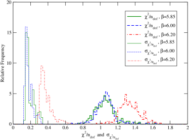
Refer to caption
Figure 4: Shown are normalized histograms of the χ2/ndofsuperscript𝜒2subscript𝑛𝑑𝑜𝑓\chi^{2}/n_{dof} (thick lines) of all the channels fit for each of our lattice spacings. To the left of the diagram one also has histograms of the standard deviation of these values, σχ2/ndofsubscript𝜎superscript𝜒2subscript𝑛𝑑𝑜𝑓\sigma_{\chi^{2}/n_{dof}} (thin lines). Smeared and unsmeared data at the same lattice spacing had essentially the same histograms so the plot does not distinguish them.

The actual source of this discrepancy can be traced to lower statistics, as our β=6.2𝛽6.2\beta=6.2 data involved only 200200200 configurations compared to 600600600 at the coarser lattice spacings. In Ref. von Hippel et al. (2008) we fit subsets of the configurations of our β=6.0𝛽6.0\beta=6.0 data to see what the effect of poor statistics would be on the result. The subfit on only 200200200 configurations shown in that paper clearly demonstrates an increase in the χ2/ndofsuperscript𝜒2subscript𝑛𝑑𝑜𝑓\chi^{2}/n_{dof} comparable to what we find here with our β=6.2𝛽6.2\beta=6.2 data. Since our poorer β=6.2𝛽6.2\beta=6.2 fits can be explained by fewer statistics, we conclude that where good fits to the data exist they are found by the fitting algorithm. It is notable that the shape of this histogram can be used to assess the minimum number of configurations required for a proper simulation. Presumably, once a sufficient number of configurations have been used that states are reliably identified, one will get a good distribution of χ2/ndofsuperscript𝜒2subscript𝑛𝑑𝑜𝑓\chi^{2}/n_{dof} centered on one.101010Obviously the number of correlators fit in each channel varied greatly so the width of the distribution is partly related to the statistics induced by this variation. A greater number of configurations would then serve to lower the error on the states found and narrow the overall distribution.111111One may wonder why our smeared and unsmeared correlators had comparable histograms if the smeared data had to resolve a fewer number of states. Why this should be the case is likely due to the asymmetrical smearing that is done to our source and sink operators. While it is true that we are removing excited states by smearing, in our case we are producing noisier correlators with the result that our statistics remain wanting for our smeared correlators at our finest lattice spacing. Our baryon study with the same smearing showed a similar result Abdel-Rehim et al. (2006b).

Since the errors of the parameters were obtained by bootstrapping the functional form found by the evolutionary algorithm, it was also possible to calculate the variation in the χ2/ndofsuperscript𝜒2subscript𝑛𝑑𝑜𝑓\chi^{2}/n_{dof} for each fit. Figure 4 includes histograms of the standard deviation σχ2/ndofsubscript𝜎superscript𝜒2subscript𝑛𝑑𝑜𝑓\sigma_{\chi^{2}/n_{dof}} of our fits. For the coarser lattice spacings with 600600600 configurations one finds that there is a relatively narrow distribution of the χ2/ndofsuperscript𝜒2subscript𝑛𝑑𝑜𝑓\chi^{2}/n_{dof} across bootstrap configurations. This gives some confidence that the fitting algorithm has found a stable functional form for the fit. For β=6.2𝛽6.2\beta=6.2, however, the variation is found to be wider. That this is due to the fewer configurations available at this spacing can also be confirmed by consulting Ref. von Hippel et al. (2008) which shows that our subfit to 200200200 configurations displayed a similar trend. Similar findings are obtained by plotting the standard quality of fit Q𝑄Q, as discussed in Ref. Petry (2008).

Because our evolutionary algorithm fitting function was designed to fit correlators that are sums of decaying exponentials only, this causes a systematic error in the A1++superscriptsubscript𝐴1absentA_{1}^{++} channel where, due to a quenching artifact, this is not the functional form of the correlator. In quenched lattice QCD one has a ghost contribution in the scalar correlator due to the ηsuperscript𝜂\eta^{\prime}-π𝜋\pi intermediate state being light and of negative norm in this approximation Bardeen et al. (2001). In our data this effect is most pronounced at the lightest quark mass in the β=6.2𝛽6.2\beta=6.2 charged channel. See Figure 5 where our five correlators in this channel are plotted. Because we only have good C𝐶C and product PG𝑃𝐺PG in our neutral and charged channels respectively, this artifact will appear in other A1subscript𝐴1A_{1} channels Abdel-Rehim et al. (2006a). Because the coefficients in our fit functions are constrained to be positive, the effect of negative ghost contributions is primarily to produce a poor fit. Several of the higher outliers of χ2/ndofsuperscript𝜒2subscript𝑛𝑑𝑜𝑓\chi^{2}/n_{dof} in Figure 4 are readily traced to A1subscript𝐴1A_{1} channels containing this ghost contribution.
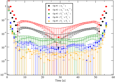
Refer to caption
Figure 5: Shown are the five unsmeared diagonal correlators for the charged A1++superscriptsubscript𝐴1absentA_{1}^{++} channel at β=6.2𝛽6.2\beta=6.2 and lightest quark mass. Solid points are positive values and open are negative. In parentheses after each number the octahedral irrep of the local quark structure and the gauge field used to generate the operator are given. The first operator has no extended gauge field structure. The last two operators use different T1superscriptsubscript𝑇1absentT_{1}^{--} local quark representations in their construction, operator #4#4\#4 using quark structure T12superscriptsubscript𝑇1limit-from2T_{1}^{2--}, with the superscript 222 indicating the multiplicity α𝛼\alpha from Table 5.

In order to evaluate the consistency of the fitting algorithm we did at least two runs in each channel and found no significant variation in the results. Where difference occurred it would tend to be a single state with large error found in a single correlator. Given a finite number of generations in a run this is to be expected.

The fitting algorithm appears to have resolved states predictably. Unsmeared channels found greater numbers of states than did smeared channels. In some channels no state was found, which affirms that the method does not claim signals in everything. Occasionally a clearly spurious state with large error would appear in a single correlator which is also expected from the statistical variation of the data itself. Finer lattice spacings in the unsmeared case found more states since a greater number of excitations could be resolved. Occasionally the β=6.2𝛽6.2\beta=6.2 lattice spacing appeared to resolve an intermediate state not seen in the other spacings. While the bifurcation of states could certainly occur at finer spacing, the fewer configurations at β=6.2𝛽6.2\beta=6.2 do not allow us to make a strong conclusion from this observation.

Occasionally states of low energy would appear in some channels with large error below the obvious ground state. Such errant signals are a consequence of fitting at Euclidean times far from the source, where correlators are noisy. They may be an artifact of time step correlation not being entirely removed through the use of the correlated χ2superscript𝜒2\chi^{2}. We regard the presence of these noisy spurious states as a reminder that we are using a true black box method: the χ2/ndofsuperscript𝜒2subscript𝑛𝑑𝑜𝑓\chi^{2}/n_{dof} is slightly reduced by their presence, and we have not prevented their appearance through human intervention such as choosing a fitting window in Euclidean time.

As found in Ref. von Hippel et al. (2008), the computer time required for an evolutionary fit scales with the number of parameters required. This depends not only on the number of states in the channel but includes the coefficients required on each correlator, and hence depends on the number of correlators fit in the channel. By smearing we reduce the number of states and therefore the number of coefficients and thus smearing allowed us to fit many correlators in the same channel quickly.

As part of the analysis we tried to fit all smeared correlators corresponding to the J=4𝐽4J=4 channel which includes all four octahedral irreps (A1subscript𝐴1A_{1}, E𝐸E, T1subscript𝑇1T_{1}, and T2subscript𝑇2T_{2}) to which its subduced representation reduces for a given PC𝑃𝐶PC. Such fits involved fitting on the order of forty correlators simultaneously and, although taking proportionately longer, were, in the end, tractable by the fitting algorithm.

VI.2 Observations on twisted mass

Figures 6 and 7 show fits with both charged and neutral operators in the A1subscript𝐴1A_{1} and T1subscript𝑇1T_{1} channels, which couple to spin zero and one respectively in the continuum. Results at four different degenerate quark masses are shown. The sizes of the points are scaled to give a qualitative impression of the significance of the state in the datasets via the factor:

2πarctan(1Ni=1NZ(i)ϵ(i)).2𝜋1𝑁superscriptsubscript𝑖1𝑁superscript𝑍𝑖superscriptitalic-ϵ𝑖\frac{2}{\pi}\arctan\left(\frac{1}{N}\sum_{i=1}^{N}\frac{Z^{(i)}}{\epsilon^{(i)}}\right)\;. (41)

Here N𝑁N is the number of correlators involved in the fit, Z(i)superscript𝑍𝑖Z^{(i)} is the coefficient on the ithsuperscript𝑖𝑡i^{th} correlator for the given energy state (taken to be zero if there was no coefficient found on that dataset) and ϵ(i)superscriptitalic-ϵ𝑖\epsilon^{(i)} is the bootstrap error of the given coefficient. The arctan\arctan function is used to ensure the scale factor ranges from 00 to 111. The utility of the scaling is that it facilitates the identification of the same state across lattice spacings and quark masses for extrapolation purposes. The scale factor is not numerically involved in any extrapolation however.
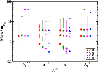
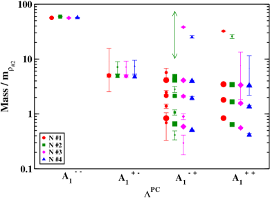
Refer to caption
Refer to caption
Figure 6: The results of the fits to the four A1subscript𝐴1A_{1} channels at β=5.85𝛽5.85\beta=5.85 for the unsmeared correlators. For each of the charged (C) and neutral (N) channels, there are four fits for the quark masses going from the heaviest (mass #1#1\#1) to the lightest (mass #4#4\#4). Points are scaled to the ρ𝜌\rho mass found in the smeared charged mass #2#2\#2 channel. Point sizes are scaled to reflect their significance as given by Equation (41).
Refer to caption
Refer to caption
Figure 7: The results of the fits to the four T1subscript𝑇1T_{1} channels at β=5.85𝛽5.85\beta=5.85 for the unsmeared correlators. Notation is identical with Figure 6.

In Figures 6 and 7, one is able to see easily the effect of the twisted mass channel contamination discussed in Section III. In Figure 6 the ground state pseudoscalar (“pion”) is clearly visible across quark masses where it should be in the A1+superscriptsubscript𝐴1absentA_{1}^{-+} channel for both the charged and neutral correlators. For the charged operators, channels are expected to contaminate others with the same PG𝑃𝐺PG product. The charged pion shows up clearly as contamination in the A1+superscriptsubscript𝐴1absentA_{1}^{+-} channel as predicted. That it is contamination is clear not only because there is no corresponding signal in the neutral channel but also the larger error and smaller symbols are both indicative of a weaker signal than the authentic one in the A1+superscriptsubscript𝐴1absentA_{1}^{-+} channel. Comparison of the A1++superscriptsubscript𝐴1absentA_{1}^{++} channel with the A1superscriptsubscript𝐴1absentA_{1}^{--} channel similarly shows contamination of the authentic scalar A1++superscriptsubscript𝐴1absentA_{1}^{++} ground state signal in its twinned channel.

Turning to the neutral case, charge conjugation is respected and one sees the pion now contaminating the A1++superscriptsubscript𝐴1absentA_{1}^{++} channel. States in the latter channel in turn are contaminating the A1+superscriptsubscript𝐴1absentA_{1}^{-+} channel where one clearly sees weak contamination states interspersed with authentic states. It is a testament to the fitting algorithm that it is able to distinguish these errant states.

The strength of the ground state vector (“ρ𝜌\rho meson”) allows us to confirm similarly the contamination relations for those channels not evident in the scalar case. The ρ𝜌\rho is clearly identified in both charged and neutral T1superscriptsubscript𝑇1absentT_{1}^{--} channels in Figure 7. Consideration of the contamination in the charged channel suggests the particle should appear in the T1++superscriptsubscript𝑇1absentT_{1}^{++} channel, which it clearly does. In the neutral case the ρ𝜌\rho contamination is appearing in the T1+superscriptsubscript𝑇1absentT_{1}^{+-} channel as expected. It is worth noting that contamination states are not appearing in unexpected channels. The strength of the pion and the ρ𝜌\rho as signals, even in contamination, would make them easily discernible.

When contamination is weak or when the actual states in the channel being contaminated are themselves weak one may see distortions in the actual state if the two states are nearby or cannot be distinguished. Higher statistics are required to disentangle correctly the greater number of states that will appear in a given channel. The value of being able to compare neutral and charged channels which get contaminated differently is readily apparent.

Overall, contamination appears to decrease with finer lattice spacing. At lighter quark mass the contamination also lessens but so does the actual signal in the original channel. In our simulation, smearing reduced the contamination strength and in our smeared fits it was only possible to identify reliably ground state ρ𝜌\rho and pion contamination. The decrease in contamination with lattice spacing and the effect of smearing can be seen in the fit plots in Section VI.3. The fits in Figures 6 and 7, being to data both unsmeared and at our coarsest lattice spacing, are for illustration of the contamination effect. The smeared data we actually fit for our results appear to have limited contamination identified by the fitting algorithm.

VI.3 Meson spectroscopy

The data from the smeared T1superscriptsubscript𝑇1absentT_{1}^{--} and T1+superscriptsubscript𝑇1absentT_{1}^{-+} channels are provided in Figures 8 and 9 respectively. The sizes of all data points are scaled by Eq. (41) so tiny points are often devoid of any physics content. Similar plots for all other ΛPCsuperscriptΛ𝑃𝐶\Lambda^{PC} appear in Ref. Petry (2008).

Refer to caption
Refer to caption
Figure 8: Fits to smeared T1superscriptsubscript𝑇1absentT_{1}^{--} correlators are shown. Experimental measurements Yao et al. (2006) are plotted for comparison.
Refer to caption
Refer to caption
Figure 9: Fits to smeared T1+superscriptsubscript𝑇1absentT_{1}^{-+} correlators are shown. A clear signal appears between 222 and 333 GeV which has been extrapolated. The lower points seem to suggest that the fitting algorithm is detecting some other state, likely channel contamination due to tmLQCD. This is an exotic channel. Experimental claims Yao et al. (2006) are plotted for comparison.

In Figure 8, the extrapolated ground state vector meson (the ρ𝜌\rho) is in agreement with its physical value, and a single excited state is resolved. The neutral β=5.85𝛽5.85\beta=5.85 excited state, while present at every quark mass, appears to be interfering with the ground state. The resulting poor chiral extrapolations of the neutral β=5.85𝛽5.85\beta=5.85 data will be excluded from the continuum extrapolation of both the ground and excited states. At the heaviest quark mass the ground state for the neutral β=6.0𝛽6.0\beta=6.0 fit is bifurcated (the points are indistinguishable on this plot) presumably because statistical variation made this a slightly more probable fit. Due to limited statistics in the β=6.2𝛽6.2\beta=6.2 channel (recall Section VI.1), there may be increased systematic errors that arise during the fitting at β=6.2𝛽6.2\beta=6.2. One might therefore prefer to omit β=6.2𝛽6.2\beta=6.2 data from continuum extrapolations.

In Figure 9, results in the exotic T1+superscriptsubscript𝑇1absentT_{1}^{-+} channel are plotted. A clear signal is evident between 2 and 3 GeV, while tiny points also appear in the small mass range. These tiny points may be attributed in part to contamination with the other T1subscript𝑇1T_{1} channels due to tmLQCD’s symmetry structure, and in part to statistical variation within the fitting procedure. At our largest quark mass, which is approximately the strange quark mass, our results are consistent with the lattice study of Ref. Lacock et al. (1996) which used displaced quarks to generate angular momenta in the operators for quenched simulations at β=6.0𝛽6.0\beta=6.0.

The results of all our simulations, after linear chiral extrapolations, are given in Table 14 along with continuum extrapolations. Extrapolations that omit the β=6.2𝛽6.2\beta=6.2 data, i.e. simple averages of data at the other two β𝛽\beta values, are provided in Table 15 for all ΛPCsuperscriptΛ𝑃𝐶\Lambda^{PC}. The predictions for charged meson masses are also shown graphically in Figure 10, together with the experimental mass spectrum.

Table 14: Extrapolations of each resolved channel labeled by its irrep (ΛPCsuperscriptΛ𝑃𝐶\Lambda^{PC}) and its type, charged (C) or neutral (N), are given. States designated by an asterisk indicate a higher energy state in the same channel. The inferred continuum quantum number J𝐽J of the state is also given. Chiral extrapolations (linear) for each β𝛽\beta are shown along with their χ2/ndofsuperscript𝜒2subscript𝑛𝑑𝑜𝑓\chi^{2}/n_{dof} in subsequent columns. The continuum extrapolation of these results is shown in the last column. We have omitted the pion (A1+superscriptsubscript𝐴1absentA_{1}^{-+}) from the table. All energies are in GeV.
Channel β=5.85𝛽5.85\beta=5.85 β=6.0𝛽6.0\beta=6.0 β=6.2𝛽6.2\beta=6.2 Final
Irrep(s) J C/N Energy χ2/νsuperscript𝜒2𝜈\chi^{2}/\nu Energy χ2/νsuperscript𝜒2𝜈\chi^{2}/\nu Energy χ2/νsuperscript𝜒2𝜈\chi^{2}/\nu Energy χ2/νsuperscript𝜒2𝜈\chi^{2}/\nu
A1++superscriptsubscript𝐴1absentA_{1}^{++} 0 C 1.35(3)1.3531.35(3) 1.5791.5791.579 1.36(3)1.3631.36(3) 0.1310.1310.131 1.40(6)1.4061.40(6) 0.0150.0150.015 1.40(6)1.4061.40(6) 0.2310.2310.231
N 1.01(4)1.0141.01(4) 2.5662.5662.566 1.21(4)1.2141.21(4) 0.1980.1980.198 1.20(8)1.2081.20(8) 0.0120.0120.012 1.39(8)1.3981.39(8) 1.6831.6831.683
A1+superscriptsubscript𝐴1absentA_{1}^{+-} 0 C 3.3(3)3.333.3(3) 0.0150.0150.015 4.2(4)4.244.2(4) 1.5761.5761.576 5.1(10)5.1105.1(10) 0.0230.0230.023 5.6(8)5.685.6(8) 0.0530.0530.053
N 3.5(4)3.543.5(4) 0.6880.6880.688 2.5(3)2.532.5(3) 0.0140.0140.014 3.1(6)3.163.1(6) 0.1940.1940.194 2.1(7)2.172.1(7) 2.2092.2092.209
A1+superscriptsubscript𝐴1absentA_{1}^{*-+} 0 C 0.31(17)0.31170.31(17) 2.8152.8152.815 1.96(18)1.96181.96(18) 0.0480.0480.048 2.08(10)2.08102.08(10) 0.3030.3030.303 2.2(3)2.232.2(3)111Continuum extrapolation excluded β=5.85𝛽5.85\beta=5.85 data point. ...
N 1.47(16)1.47161.47(16) 0.0270.0270.027 1.69(10)1.69101.69(10) 0.2680.2680.268 1.96(13)1.96131.96(13) 1.5481.5481.548 2.14(19)2.14192.14(19) 0.3090.3090.309
T1++superscriptsubscript𝑇1absentT_{1}^{++} 1 C 0.98(5)0.9850.98(5) 0.3710.3710.371 1.25(5)1.2551.25(5) 0.9900.9900.990 1.6(2)1.621.6(2) 0.3760.3760.376 1.65(12)1.65121.65(12) 0.4610.4610.461
N 1.33(2)1.3321.33(2) 0.1010.1010.101 1.428(17)1.428171.428(17) 0.0030.0030.003 1.52(10)1.52101.52(10) 0.0100.0100.010 1.57(5)1.5751.57(5) 0.0610.0610.061
T1++superscriptsubscript𝑇1absentT_{1}^{*++} 1 C 2.4(3)2.432.4(3) 0.8430.8430.843 2.3(3)2.332.3(3) 0.2130.2130.213 3.3(6)3.363.3(6) 0.3150.3150.315 2.9(6)2.962.9(6) 1.6881.6881.688
N 3.0(7)3.073.0(7) 0.1090.1090.109 2.4(3)2.432.4(3) 0.2980.2980.298 5.8(13)5.8135.8(13) 0.4590.4590.459 2.9(10)2.9102.9(10) 7.2837.2837.283
T1+superscriptsubscript𝑇1absentT_{1}^{+-} 1 C 1.40(3)1.4031.40(3) 1.5071.5071.507 1.48(3)1.4831.48(3) 1.0181.0181.018 1.74(8)1.7481.74(8) 0.9610.9610.961 1.69(7)1.6971.69(7) 4.1364.1364.136
N 1.14(6)1.1461.14(6) 0.7150.7150.715 1.62(6)1.6261.62(6) 0.0180.0180.018 1.57(7)1.5771.57(7) 0.1990.1990.199 1.90(10)1.90101.90(10) 6.7286.7286.728
T1+superscriptsubscript𝑇1absentT_{1}^{*+-} 1 C 2.6(4)2.642.6(4) 1.0951.0951.095 2.7(3)2.732.7(3) 0.5350.5350.535 2.8(6)2.862.8(6) 0.0110.0110.011 2.9(7)2.972.9(7) 0.0070.0070.007
N 3.1(4)3.143.1(4) 0.2830.2830.283 2.8(4)2.842.8(4) 0.0210.0210.021 3.2(4)3.243.2(4) 1.8331.8331.833 3.1(6)3.163.1(6) 0.5910.5910.591
T1+superscriptsubscript𝑇1absentT_{1}^{-+} 1 C 1.80(18)1.80181.80(18) 0.7740.7740.774 2.15(18)2.15182.15(18) 0.0080.0080.008 2.4(4)2.442.4(4) 0.2580.2580.258 2.7(4)2.742.7(4) 0.0220.0220.022
N 1.7(2)1.721.7(2) 0.5660.5660.566 2.3(2)2.322.3(2) 0.0270.0270.027 2.9(5)2.952.9(5) 0.0000.0000.000 3.3(5)3.353.3(5) 0.1570.1570.157
T1superscriptsubscript𝑇1absentT_{1}^{--} 1 C 0.767(19)0.767190.767(19) 0.1410.1410.141 0.764(16)0.764160.764(16) 0.0360.0360.036 0.79(3)0.7930.79(3) 0.0660.0660.066 0.78(3)0.7830.78(3) 0.5730.5730.573
N 0.797(6)0.79760.797(6) 0.5080.5080.508 0.812(12)0.812120.812(12) 0.5150.5150.515 0.80(2)0.8020.80(2) 0.1220.1220.122 0.79(5)0.7950.79(5)111Continuum extrapolation excluded β=5.85𝛽5.85\beta=5.85 data point. ...
T1superscriptsubscript𝑇1absentT_{1}^{*--} 1 C 1.18(12)1.18121.18(12) 0.0060.0060.006 1.50(7)1.5071.50(7) 0.0300.0300.030 1.82(18)1.82181.82(18) 0.0210.0210.021 2.00(19)2.00192.00(19) 0.2530.2530.253
N 0.84(2)0.8420.84(2) 3.9263.9263.926 1.63(10)1.63101.63(10) 0.1990.1990.199 1.88(16)1.88161.88(16) 0.1540.1540.154 2.2(4)2.242.2(4)111Continuum extrapolation excluded β=5.85𝛽5.85\beta=5.85 data point. ...
(E,T2)++superscript𝐸subscript𝑇2absent(E,T_{2})^{++} 2 C 0.4(2)0.420.4(2) 0.3400.3400.340 0.75(19)0.75190.75(19) 0.2900.2900.290 1.0(4)1.041.0(4) 0.2440.2440.244 1.3(4)1.341.3(4) 0.0030.0030.003
N 0.6(4)0.640.6(4) 0.0490.0490.049 0.52(13)0.52130.52(13) 0.1790.1790.179 0.5(3)0.530.5(3) 0.0510.0510.051 0.4(4)0.440.4(4) 0.0020.0020.002
(E,T2)++superscript𝐸subscript𝑇2absent(E,T_{2})^{*++} 2 C 3.7(7)3.773.7(7) 0.1960.1960.196 2.7(4)2.742.7(4) 0.0630.0630.063 2.9(9)2.992.9(9) 0.1270.1270.127 1.9(10)1.9101.9(10) 0.4680.4680.468
N 2.4(3)2.432.4(3) 2.2352.2352.235 3.0(4)3.043.0(4) 0.1030.1030.103 3.2(8)3.283.2(8) 0.0370.0370.037 3.7(8)3.783.7(8) 0.0230.0230.023
(E,T2)+superscript𝐸subscript𝑇2absent(E,T_{2})^{+-} 2 C 2.8(6)2.862.8(6) 0.0570.0570.057 2.7(4)2.742.7(4) 0.0650.0650.065 2.9(8)2.982.9(8) 0.0180.0180.018 2.8(9)2.892.8(9) 0.0660.0660.066
N 3.2(5)3.253.2(5) 0.0050.0050.005 2.9(4)2.942.9(4) 0.0310.0310.031 3.1(6)3.163.1(6) 0.0260.0260.026 2.9(8)2.982.9(8) 0.1720.1720.172
(E,T2)+superscript𝐸subscript𝑇2absent(E,T_{2})^{-+} 2 C 2.3(2)2.322.3(2) 0.3340.3340.334 2.9(4)2.942.9(4) 0.0250.0250.025 3.3(9)3.393.3(9) 0.1210.1210.121 3.7(7)3.773.7(7) 0.0010.0010.001
N 2.4(2)2.422.4(2) 4.1334.1334.133 2.8(4)2.842.8(4) 0.0010.0010.001 3.0(7)3.073.0(7) 0.3440.3440.344 3.2(7)3.273.2(7) 0.0010.0010.001
A2++superscriptsubscript𝐴2absentA_{2}^{++} 3 C 0.5(7)0.570.5(7) ... 1.8(5)1.851.8(5) 0.0020.0020.002 3.5(8)3.583.5(8) 0.0520.0520.052 4.3(10)4.3104.3(10) 0.5730.5730.573
N 0.7(4)0.740.7(4) ... 10.(8)formulae-sequence10810.(8) 0.0050.0050.005 3.2(8)3.283.2(8) 0.0170.0170.017 4.4(11)4.4114.4(11) 0.9120.9120.912
A2+superscriptsubscript𝐴2absentA_{2}^{-+} 3 C 1.3(4)1.341.3(4) 0.2300.2300.230 1.4(7)1.471.4(7) 0.6720.6720.672 1.1(6)1.161.1(6) 0.0720.0720.072 1.1(8)1.181.1(8) 0.1130.1130.113
N 1.5(5)1.551.5(5) 0.3760.3760.376 1.2(4)1.241.2(4) 0.0880.0880.088 1.2(4)1.241.2(4) 0.6640.6640.664 1.0(6)1.061.0(6) 0.0090.0090.009
Table 15: Weighted average of the chirally extrapolated β=5.85𝛽5.85\beta=5.85 and β=6.0𝛽6.0\beta=6.0 lattice spacing results of each resolved channel labeled by its irrep (ΛPCsuperscriptΛ𝑃𝐶\Lambda^{PC}) and its type (charged or neutral) are given. States designated by an asterisk indicate a higher energy state in the same channel. The inferred continuum quantum number J𝐽J of the state is also given. We have omitted the pion (A1+superscriptsubscript𝐴1absentA_{1}^{-+}) from the table. All energies are in GeV.
Channel Energy
Irrep(s) J        Charged        Neutral
A1++superscriptsubscript𝐴1absentA_{1}^{++} 0 1.353(19)1.353191.353(19) 1.12(3)1.1231.12(3)
A1+superscriptsubscript𝐴1absentA_{1}^{+-} 0 3.6(2)3.623.6(2) 2.9(3)2.932.9(3)
A1+superscriptsubscript𝐴1absentA_{1}^{*-+} 0 1.96(18)1.96181.96(18)111Excluded β=5.85𝛽5.85\beta=5.85 data point. 1.63(8)1.6381.63(8)
T1++superscriptsubscript𝑇1absentT_{1}^{++} 1 1.12(3)1.1231.12(3) 1.394(14)1.394141.394(14)
T1++superscriptsubscript𝑇1absentT_{1}^{*++} 1 2.4(2)2.422.4(2) 2.5(2)2.522.5(2)
T1+superscriptsubscript𝑇1absentT_{1}^{+-} 1 1.44(2)1.4421.44(2) 1.37(4)1.3741.37(4)
T1+superscriptsubscript𝑇1absentT_{1}^{*+-} 1 2.7(2)2.722.7(2) 2.9(3)2.932.9(3)
T1+superscriptsubscript𝑇1absentT_{1}^{-+} 1 1.98(13)1.98131.98(13) 1.98(16)1.98161.98(16)
T1superscriptsubscript𝑇1absentT_{1}^{--} 1 0.765(12)0.765120.765(12) 0.812(12)0.812120.812(12)111Excluded β=5.85𝛽5.85\beta=5.85 data point.
T1superscriptsubscript𝑇1absentT_{1}^{*--} 1 1.42(6)1.4261.42(6) 1.63(10)1.63101.63(10)111Excluded β=5.85𝛽5.85\beta=5.85 data point.
(E,T2)++superscript𝐸subscript𝑇2absent(E,T_{2})^{++} 2 0.61(15)0.61150.61(15) 0.53(13)0.53130.53(13)
(E,T2)++superscript𝐸subscript𝑇2absent(E,T_{2})^{*++} 2 2.9(3)2.932.9(3) 2.6(3)2.632.6(3)
(E,T2)+superscript𝐸subscript𝑇2absent(E,T_{2})^{+-} 2 2.8(3)2.832.8(3) 3.0(3)3.033.0(3)
(E,T2)+superscript𝐸subscript𝑇2absent(E,T_{2})^{-+} 2 2.46(19)2.46192.46(19) 2.52(20)2.52202.52(20)
A2++superscriptsubscript𝐴2absentA_{2}^{++} 3 1.3(4)1.341.3(4) 0.7(4)0.740.7(4)
A2+superscriptsubscript𝐴2absentA_{2}^{-+} 3 1.3(4)1.341.3(4) 1.3(3)1.331.3(3)
Refer to caption
Figure 10: Experimental values Yao et al. (2006) of light unflavored mesons (squares) in the isovector channel for each JPCsuperscript𝐽𝑃𝐶J^{PC} are compared to the results of this simulation (diamonds) that are the weighted average over lattice spacings β=5.85𝛽5.85\beta=5.85 and β=6.0𝛽6.0\beta=6.0 extrapolated to zero quark mass.

Note that our results from the heaviest quark mass at β=6.0𝛽6.0\beta=6.0 (provided explicitly in Ref. Petry (2008)) can be compared directly to Ref. Lacock et al. (1996), and good agreement is found for the available channels: a0subscript𝑎0a_{0}, π𝜋\pi, ρ𝜌\rho, b1subscript𝑏1b_{1}, a1subscript𝑎1a_{1} and a2subscript𝑎2a_{2}. The exotic states which we identify in the 0+superscript0absent0^{+-}, 1+superscript1absent1^{-+}, and 2+superscript2absent2^{+-} channels, for the strange quark mass at β=6.0𝛽6.0\beta=6.0, are also found to be comparable to values which they ascribe to those same JPCsuperscript𝐽𝑃𝐶J^{PC}.

Our result for the 1+superscript1absent1^{-+} from Table 15 agrees well with the general consensus of quenched Lacock et al. (1996); Bernard et al. (1997); Mei and Luo (2003); Hedditch et al. (2005); Cook and Fiebig (2006) and dynamical Lacock and Schilling (1999); Bernard et al. (2003) lattice studies that the lightest exotic meson is 1+superscript1absent1^{-+} with a mass near 1.9 GeV. We also note that the flux-tube model predicts exotic hybrids 0+superscript0absent0^{+-}, 1+superscript1absent1^{-+}, and 2+superscript2absent2^{+-} near 1.91.91.9 GeV in the light isovector channel Isgur et al. (1985).

Although results of our simulations with Wilson fermions have not been reported here, they did provide independent confirmation of which signals were actually contamination that arose due to the twisted mass term.

In all but the A2subscript𝐴2A_{2} channels, the smeared operators produced better fits than unsmeared operators. For A2PCsuperscriptsubscript𝐴2𝑃𝐶A_{2}^{PC}, it was found that just fitting the smeared channel tended to produce failures in the bootstrap fits which are used to generate the errors of the parameters. The reason for this failure is poor statistics due to a combination of the relatively few correlators in each A2subscript𝐴2A_{2} channel (no row averaging occurs in a one-dimensional channel) and the weakness of the expected states in the channel since A2subscript𝐴2A_{2} couples only to continuum J3𝐽3J\geq 3 as shown in Table 2. As our motivation for fitting smeared states is to reduce the influence of high energy states and since the A2subscript𝐴2A_{2} channels have very few low lying states even in the unsmeared case, we refit all A2subscript𝐴2A_{2} correlators, both smeared and not, simultaneously. This gives sufficient statistics to make our bootstrap fits converge properly.

Visual inspection of the fits to the E𝐸E and T2subscript𝑇2T_{2} channels independently, in each PC𝑃𝐶PC combination, revealed that results were remarkably similar for any state found. This is to be expected since, by Table 2, the lowest angular momentum to which they both couple is J=2𝐽2J=2. With the assumption that the few states found across these channels are of this angular momentum, we do combined fits of all correlators of E𝐸E and T2subscript𝑇2T_{2} together for each PC𝑃𝐶PC. In these combined fits the algorithm finds the states to be statistically the same (i.e. it does not bifurcate any of the states), thus allowing us to conclude that our results are commensurate with ascribing a value J=2𝐽2J=2 to the common state.121212Technically J=4𝐽4J=4 is also a logical possibility since its subduced representation reduces to both irreps E𝐸E and T2subscript𝑇2T_{2} as well. Furthermore it allows us to use all the available data to extract its value. We thus tabulate results only for the combined (E,T2)𝐸subscript𝑇2(E,T_{2}) fits, and not them separately. Our lattice spacing is fine enough that given our statistics it is unlikely that any splitting between E𝐸E and T2subscript𝑇2T_{2} states for a common J=2𝐽2J=2 state would be detectable, and it is not.131313Such splitting can be observed across continuum subduction channels on coarser lattices. See Ref. Morningstar and Peardon (1997). The remaining states in our fits are assigned their most probable continuum J𝐽J values based on Table 2, namely J=0𝐽0J=0, 111, and 333 for irreps A1subscript𝐴1A_{1}, T1subscript𝑇1T_{1}, and A2subscript𝐴2A_{2} respectively.141414While J=3𝐽3J=3 could also appear in T1subscript𝑇1T_{1} and T2subscript𝑇2T_{2} channels as well, the likely weakness of such a signal made a combined fitting of these channels inappropriate in comparison to the J=2𝐽2J=2 case, given the presence of lower J𝐽J in T1subscript𝑇1T_{1} and T2subscript𝑇2T_{2} channels and the limitations of our statistics.

VI.4 Observations on operators

To give insight into the nature of the operators which contribute to a particular state we have produced Table LABEL:tab:irrepcontrib in Appendix A. There one finds the operators which are found to contribute to each extrapolated state, written in terms of their local quark and extended gauge field content from which they are constructed. The nature of our operators is such that only one irrep is found in any such product as shown in Table 10 so this labeling uniquely identifies the operator.

To quantify the significance of an operator’s diagonal correlator to a given channel two additional pieces of information are given in Table LABEL:tab:irrepcontrib. For each such operator the number of times it was found contributing to the state out of the twelve possible lattice spacing and quark mass combinations that were fit is given. In some cases a small contribution may not be statistically significant and as such the fitting algorithm may opt not to give a coefficient for it. Secondly, the table provides the largest magnitude of the coefficient Z𝑍Z found for that state, among those fits that had a coefficient. These latter values are scaled by their error so as to give a measure of their significance. The table is organized to give the most significant operators contributing to a channel first in the list.

Several observations may be made from Table LABEL:tab:irrepcontrib. For one, operators with a non-scalar gauge structure still contribute to ground states. For the ρ𝜌\rho meson (T1superscriptsubscript𝑇1absentT_{1}^{--} ground state) the greatest contributions come from those operators which have a quark structure of T1superscriptsubscript𝑇1absentT_{1}^{--}, either a local operator or with an extended A1++superscriptsubscript𝐴1absentA_{1}^{++} gauge field. However, as can be seen in the table, one also has a significant overlap with states of the form A1+T1+tensor-productsuperscriptsubscript𝐴1absentsuperscriptsubscript𝑇1absentA_{1}^{-+}\otimes T_{1}^{+-} in which the gauge field is actually providing the vector nature of the state.151515For the ground state pion (A1+superscriptsubscript𝐴1absentA_{1}^{-+}), not shown in Table LABEL:tab:irrepcontrib, it is to be remarked that there is similarly a clear ground state signal from the T1T1tensor-productsuperscriptsubscript𝑇1absentsuperscriptsubscript𝑇1absentT_{1}^{--}\otimes T_{1}^{--} operators. The excited state T1superscriptsubscript𝑇1absentT_{1}^{*--} shows, on the other hand, a much greater relative contribution from the vector gauge field operators, but still dominant contributions from the vector quark operators. For the ground states T1++superscriptsubscript𝑇1absentT_{1}^{++} and T1+superscriptsubscript𝑇1absentT_{1}^{+-} the operators with quark vector structure dominate, however for their excited T1++superscriptsubscript𝑇1absentT_{1}^{*++} and T1+superscriptsubscript𝑇1absentT_{1}^{*+-} states it is seen that a greater contribution comes from the operators with vector gauge field structure. This observation is an example of how lattice studies of the spectrum can inform discussion of the distinction between hybrid vector mesons and conventional vector mesons which is made in models like the flux-tube model Close (1995).

Table LABEL:tab:irrepcontrib also grants further insight into the geometry of related states. In the constituent quark model, for instance, the a0subscript𝑎0a_{0}, a1subscript𝑎1a_{1}, and b1subscript𝑏1b_{1} states belong to a common P-wave and hence are considered to share common angular momentum Lacock et al. (1996). If one looks at the main contribution to these states in their corresponding octahedral channels, A1++superscriptsubscript𝐴1absentA_{1}^{++}, T1++superscriptsubscript𝑇1absentT_{1}^{++}, and T1+superscriptsubscript𝑇1absentT_{1}^{-+} respectively, it is observed that after the local operators the main contributor in each of these channels is of the form XPCT1+tensor-productsuperscript𝑋𝑃𝐶superscriptsubscript𝑇1absentX^{PC}\otimes T_{1}^{+-}, where XPCsuperscript𝑋𝑃𝐶X^{PC} is whatever local spin structure is required to produce the correct channel. This suggests that just as common spatial angular momenta (L=1𝐿1L=1) are traditionally considered to unite these channels, so too does similar gauge field structure.

For those states we identified as J=2𝐽2J=2 with our common fits to E𝐸E and T2subscript𝑇2T_{2} channels, Table LABEL:tab:irrepcontrib shows further affirmation of this identification. In the continuum, five J=2𝐽2J=2 operators can be formed with the coupling of a J=1𝐽1J=1 quark and J=1𝐽1J=1 gauge field structure. On the lattice these five states still appear in a coupling of T1subscript𝑇1T_{1} quark and T1subscript𝑇1T_{1} gauge field, but now in the subduction of J=2𝐽2J=2 as a two-dimensional E𝐸E irrep and a three-dimensional T2subscript𝑇2T_{2} irrep. As such one expects these E𝐸E and T2subscript𝑇2T_{2} operators produced via T1T1tensor-productsubscript𝑇1subscript𝑇1T_{1}\otimes T_{1} corresponding to an actual J=2𝐽2J=2 state to have similar properties.161616However, since one is row averaging over three operators in the T2subscript𝑇2T_{2} case compared to two in the E𝐸E case the correspondence is not expected to be identical due to differing statistics. A consideration of our eight (E,T2)𝐸subscript𝑇2(E,T_{2}) common fits shows that the contributions of such E𝐸E operators (denoted by T1T1tensor-productsubscript𝑇1subscript𝑇1T_{1}\otimes T_{1}) have comparable counts and significance to their related T2subscript𝑇2T_{2} operators (denoted by T1¯T1subscript𝑇1¯tensor-productsubscript𝑇1T_{1}\overline{\otimes}T_{1}) in all cases. Only in the comparably weak 2++superscript2absent2^{++} ground state fit, and there only in the neutral channel, is the pattern less obvious. For all these states the importance of the gluonic degrees of freedom is readily apparent, in contradistinction to the limitations imposed by a simple quark model for two local quarks.

VII Conclusion

Simulations with twisted mass lattice QCD (tmLQCD) have been used to explore the spectrum of mesons having all possible values of angular momentum, spin, and parity. Numerical results are consistent with those obtained by other authors using other lattice actions. As seen in Figure 10, we are still far from seeing the number of mesons claimed experimentally, and uncertainties are still large, but a viable methodology has been put into place. In particular, questions related to the appropriateness of tmLQCD for this physics can now be answered, the usefulness of operators containing local quark and anti-quark fields can be evaluated, and the valuable qualities of an evolutionary fitting method can be confirmed.

Because tmLQCD breaks the parity symmetry of the strong interactions, it is not clear a priori whether it can be used to determine the spectrum of hadrons having definite quantum numbers JPCsuperscript𝐽𝑃𝐶J^{PC}, which appear as ΛPCsuperscriptΛ𝑃𝐶\Lambda^{PC} on a discrete lattice. In the case of both isovector and isoscalar mesons, we have identified orthogonality relations among certain operators which are valid in tmLQCD for any chosen twist angle. We have also emphasized that some states cannot be separated, such as Λ++,ΛsuperscriptΛabsentsuperscriptΛabsent\Lambda^{++},\Lambda^{--} in the isovector case and Λ++,Λ+superscriptΛabsentsuperscriptΛabsent\Lambda^{++},\Lambda^{-+} in the isoscalar case. Nevertheless, simultaneous fits to multiple correlators allow the complete spectrum to be obtained (as proposed in Ref. Frezzotti and Rossi (2004)), and comparison of the isovector spectrum with its isoscalar counterpart serves to clarify the PC𝑃𝐶PC quantum numbers of the states. During this work, simulations with the Wilson action were performed also in order to confirm these claims.

Meson operators that require only one quark propagator, i.e. operators with a common local source for mass-degenerate quark and anti-quark, minimize computational expense. Connecting the quark and anti-quark to spatially extended gauge fields permitted all possible meson quantum numbers, but how well do these operators overlap with the physical states of QCD? Our numerical explorations produced signals for both conventional and exotic mesons. The strength of each operator’s overlap was tabulated, so that future studies can make informed choices of operators for the various meson channels. Gauge field smearing was included at source and sink, while quark field smearing was performed only at the sink.

The use of an evolutionary fitting algorithm avoided the danger of human bias during data analysis. The algorithm was able to fit multiple correlators simultaneously, with some states shared (or not) across data sets. The algorithm itself determined how many states were present based on statistical signficance, and all time steps beyond the source were included in all fits. Survival of the fittest was defined to mean minimizing χ2/ndofsuperscript𝜒2subscript𝑛𝑑𝑜𝑓\chi^{2}/n_{dof}. The algorithm even served to alert us to a case of insufficient statistics in one ensemble of lattices; this information appeared as larger χ2/ndofsuperscript𝜒2subscript𝑛𝑑𝑜𝑓\chi^{2}/n_{dof} values output from the fit, which could only be reduced toward unity by increased statistics.

Based on this work, we conclude that a detailed study of the full meson spectrum using tmLQCD is feasible. However, to obtain precise results, substantially more configurations would be required than we have used, and additional classes of operators should be considered. Quark smearing at the source, to match the sink, should improve the signal-to-noise ratio. With more precise meson mass determinations at a few β𝛽\beta values, one could see directly whether the continuum extrapolation of tmLQCD offers a significant advantage over other lattice actions, commensurate with the drawback of tmLQCD’s lack of parity conservation. It would also be interesting to consider the viability of using tmLQCD for a thorough study of the baryon spectrum.

Appendix A Operator contribution

The operators contributing to each extrapolated state are listed in Table LABEL:tab:irrepcontrib. Operators are identified by the direct product of quark local irrep and extended gauge field irrep from which they are projected, ΛfαfPfCfΛuPuCutensor-productsuperscriptsubscriptΛ𝑓subscript𝛼𝑓subscript𝑃𝑓subscript𝐶𝑓superscriptsubscriptΛ𝑢subscript𝑃𝑢subscript𝐶𝑢\Lambda_{f}^{{\alpha}_{f}P_{f}C_{f}}\otimes\Lambda_{u}^{P_{u}C_{u}}. Operators without an extended gauge structure given are local quark operators. Quark irreps from the second multiplicity have a superscript 222. In the case of the (E,T2)𝐸subscript𝑇2(E,T_{2}) fits we designate T2subscript𝑇2T_{2} operators with an ¯¯tensor-product\overline{\otimes} and E𝐸E operators with tensor-product\otimes. In the A2subscript𝐴2A_{2} fits where both smeared and unsmeared correlators were fit the unsmeared correlators are distinguished similarly with ¯¯tensor-product\overline{\otimes}. After each operator the number of lattice spacing-quark mass channels in which a coefficient was identified for the state is given (maximum 121212) followed by the maximum value of the coefficient Z𝑍Z divided by its error over those channels.

Table 16: Table of operators contributing to each extrapolated state.
Channel
Irrep(s) C/N Contributing Operators
A1++superscriptsubscript𝐴1absentA_{1}^{++} C A1++(12,95.2)superscriptsubscript𝐴1absent1295.2A_{1}^{++}(12,95.2)A1++A1++(12,94.6)tensor-productsuperscriptsubscript𝐴1absentsuperscriptsubscript𝐴1absent1294.6A_{1}^{++}\otimes A_{1}^{++}(12,94.6)T1+T1+(7,3.97)tensor-productsuperscriptsubscript𝑇1absentsuperscriptsubscript𝑇1absent73.97T_{1}^{+-}\otimes T_{1}^{+-}(7,3.97)T12T1(2,2.49)tensor-productsuperscriptsubscript𝑇1limit-from2superscriptsubscript𝑇1absent22.49T_{1}^{2--}\otimes T_{1}^{--}(2,2.49)
N A1++A1++(12,48.4)tensor-productsuperscriptsubscript𝐴1absentsuperscriptsubscript𝐴1absent1248.4A_{1}^{++}\otimes A_{1}^{++}(12,48.4)A1++(12,48.1)superscriptsubscript𝐴1absent1248.1A_{1}^{++}(12,48.1)T1+T1+(9,4.34)tensor-productsuperscriptsubscript𝑇1absentsuperscriptsubscript𝑇1absent94.34T_{1}^{+-}\otimes T_{1}^{+-}(9,4.34)T12T1(3,3.92)tensor-productsuperscriptsubscript𝑇1limit-from2superscriptsubscript𝑇1absent33.92T_{1}^{2--}\otimes T_{1}^{--}(3,3.92)
A1+superscriptsubscript𝐴1absentA_{1}^{+-} C A1+(12,9.25)superscriptsubscript𝐴1absent129.25A_{1}^{+-}(12,9.25)A1+A1++(12,9.25)tensor-productsuperscriptsubscript𝐴1absentsuperscriptsubscript𝐴1absent129.25A_{1}^{+-}\otimes A_{1}^{++}(12,9.25)T1++T1+(10,5.74)tensor-productsuperscriptsubscript𝑇1absentsuperscriptsubscript𝑇1absent105.74T_{1}^{++}\otimes T_{1}^{+-}(10,5.74)T12T1+(7,4.60)tensor-productsuperscriptsubscript𝑇1limit-from2superscriptsubscript𝑇1absent74.60T_{1}^{2--}\otimes T_{1}^{-+}(7,4.60),
T1T1+(4,4.41)tensor-productsuperscriptsubscript𝑇1absentsuperscriptsubscript𝑇1absent44.41T_{1}^{--}\otimes T_{1}^{-+}(4,4.41)
N A1+(12,5.26)superscriptsubscript𝐴1absent125.26A_{1}^{+-}(12,5.26)A1+A1++(12,5.20)tensor-productsuperscriptsubscript𝐴1absentsuperscriptsubscript𝐴1absent125.20A_{1}^{+-}\otimes A_{1}^{++}(12,5.20)T1++T1+(11,4.19)tensor-productsuperscriptsubscript𝑇1absentsuperscriptsubscript𝑇1absent114.19T_{1}^{++}\otimes T_{1}^{+-}(11,4.19)T1T1+(5,3.11)tensor-productsuperscriptsubscript𝑇1absentsuperscriptsubscript𝑇1absent53.11T_{1}^{--}\otimes T_{1}^{-+}(5,3.11),
T12T1+(2,1.30)tensor-productsuperscriptsubscript𝑇1limit-from2superscriptsubscript𝑇1absent21.30T_{1}^{2--}\otimes T_{1}^{-+}(2,1.30)
A1+superscriptsubscript𝐴1absentA_{1}^{*-+} C A1+(8,29.5)superscriptsubscript𝐴1absent829.5A_{1}^{-+}(8,29.5)A1+A1++(8,28.9)tensor-productsuperscriptsubscript𝐴1absentsuperscriptsubscript𝐴1absent828.9A_{1}^{-+}\otimes A_{1}^{++}(8,28.9)T1T1+(8,11.3)tensor-productsuperscriptsubscript𝑇1absentsuperscriptsubscript𝑇1absent811.3T_{1}^{--}\otimes T_{1}^{+-}(8,11.3)T12T1+(8,3.57)tensor-productsuperscriptsubscript𝑇1limit-from2superscriptsubscript𝑇1absent83.57T_{1}^{2--}\otimes T_{1}^{+-}(8,3.57),
T1+T1(4,9.21)tensor-productsuperscriptsubscript𝑇1absentsuperscriptsubscript𝑇1absent49.21T_{1}^{+-}\otimes T_{1}^{--}(4,9.21)A12+(4,3.11)superscriptsubscript𝐴1limit-from243.11A_{1}^{2-+}(4,3.11)T1++T1+(4,0.92)tensor-productsuperscriptsubscript𝑇1absentsuperscriptsubscript𝑇1absent40.92T_{1}^{++}\otimes T_{1}^{-+}(4,0.92)A12+A1++(3,3.46)tensor-productsuperscriptsubscript𝐴1limit-from2superscriptsubscript𝐴1absent33.46A_{1}^{2-+}\otimes A_{1}^{++}(3,3.46)
N A1+A1++(12,26.9)tensor-productsuperscriptsubscript𝐴1absentsuperscriptsubscript𝐴1absent1226.9A_{1}^{-+}\otimes A_{1}^{++}(12,26.9)A1+(12,26.9)superscriptsubscript𝐴1absent1226.9A_{1}^{-+}(12,26.9)A12+A1++(10,5.53)tensor-productsuperscriptsubscript𝐴1limit-from2superscriptsubscript𝐴1absent105.53A_{1}^{2-+}\otimes A_{1}^{++}(10,5.53)T12T1+(8,3.26)tensor-productsuperscriptsubscript𝑇1limit-from2superscriptsubscript𝑇1absent83.26T_{1}^{2--}\otimes T_{1}^{+-}(8,3.26),
A12+(7,5.58)superscriptsubscript𝐴1limit-from275.58A_{1}^{2-+}(7,5.58)T1+T1(6,4.38)tensor-productsuperscriptsubscript𝑇1absentsuperscriptsubscript𝑇1absent64.38T_{1}^{+-}\otimes T_{1}^{--}(6,4.38)T1T1+(5,5.08)tensor-productsuperscriptsubscript𝑇1absentsuperscriptsubscript𝑇1absent55.08T_{1}^{--}\otimes T_{1}^{+-}(5,5.08)T1++T1+(4,4.92)tensor-productsuperscriptsubscript𝑇1absentsuperscriptsubscript𝑇1absent44.92T_{1}^{++}\otimes T_{1}^{-+}(4,4.92)
T1++superscriptsubscript𝑇1absentT_{1}^{++} C T1++A1++(11,36.8)tensor-productsuperscriptsubscript𝑇1absentsuperscriptsubscript𝐴1absent1136.8T_{1}^{++}\otimes A_{1}^{++}(11,36.8)T1++(11,36.7)superscriptsubscript𝑇1absent1136.7T_{1}^{++}(11,36.7)T1+T1+(7,2.47)tensor-productsuperscriptsubscript𝑇1absentsuperscriptsubscript𝑇1absent72.47T_{1}^{+-}\otimes T_{1}^{+-}(7,2.47)T1+E+(7,2.00)tensor-productsuperscriptsubscript𝑇1absentsuperscript𝐸absent72.00T_{1}^{+-}\otimes E^{+-}(7,2.00),
T1T2(3,2.14)tensor-productsuperscriptsubscript𝑇1absentsuperscriptsubscript𝑇2absent32.14T_{1}^{--}\otimes T_{2}^{--}(3,2.14)T12T2(3,2.12)tensor-productsuperscriptsubscript𝑇1limit-from2superscriptsubscript𝑇2absent32.12T_{1}^{2--}\otimes T_{2}^{--}(3,2.12)A1+T1+(3,1.32)tensor-productsuperscriptsubscript𝐴1absentsuperscriptsubscript𝑇1absent31.32A_{1}^{+-}\otimes T_{1}^{+-}(3,1.32)T12T1(2,1.45)tensor-productsuperscriptsubscript𝑇1limit-from2superscriptsubscript𝑇1absent21.45T_{1}^{2--}\otimes T_{1}^{--}(2,1.45),
T1T1(2,1.39)tensor-productsuperscriptsubscript𝑇1absentsuperscriptsubscript𝑇1absent21.39T_{1}^{--}\otimes T_{1}^{--}(2,1.39)T1++T2++(2,0.60)tensor-productsuperscriptsubscript𝑇1absentsuperscriptsubscript𝑇2absent20.60T_{1}^{++}\otimes T_{2}^{++}(2,0.60)T1++E++(1,1.42)tensor-productsuperscriptsubscript𝑇1absentsuperscript𝐸absent11.42T_{1}^{++}\otimes E^{++}(1,1.42)
N T1++A1++(12,61.8)tensor-productsuperscriptsubscript𝑇1absentsuperscriptsubscript𝐴1absent1261.8T_{1}^{++}\otimes A_{1}^{++}(12,61.8)T1++(12,50.0)superscriptsubscript𝑇1absent1250.0T_{1}^{++}(12,50.0)T1+T1+(8,5.43)tensor-productsuperscriptsubscript𝑇1absentsuperscriptsubscript𝑇1absent85.43T_{1}^{+-}\otimes T_{1}^{+-}(8,5.43)T1+E+(7,3.54)tensor-productsuperscriptsubscript𝑇1absentsuperscript𝐸absent73.54T_{1}^{+-}\otimes E^{+-}(7,3.54),
T12T1(7,1.69)tensor-productsuperscriptsubscript𝑇1limit-from2superscriptsubscript𝑇1absent71.69T_{1}^{2--}\otimes T_{1}^{--}(7,1.69)A1+T1+(6,1.97)tensor-productsuperscriptsubscript𝐴1absentsuperscriptsubscript𝑇1absent61.97A_{1}^{+-}\otimes T_{1}^{+-}(6,1.97)T12T2(5,4.16)tensor-productsuperscriptsubscript𝑇1limit-from2superscriptsubscript𝑇2absent54.16T_{1}^{2--}\otimes T_{2}^{--}(5,4.16)T1T1(5,2.98)tensor-productsuperscriptsubscript𝑇1absentsuperscriptsubscript𝑇1absent52.98T_{1}^{--}\otimes T_{1}^{--}(5,2.98),
T1T2(5,0.80)tensor-productsuperscriptsubscript𝑇1absentsuperscriptsubscript𝑇2absent50.80T_{1}^{--}\otimes T_{2}^{--}(5,0.80)T1++E++(2,0.69)tensor-productsuperscriptsubscript𝑇1absentsuperscript𝐸absent20.69T_{1}^{++}\otimes E^{++}(2,0.69)T1++T2++(1,0.77)tensor-productsuperscriptsubscript𝑇1absentsuperscriptsubscript𝑇2absent10.77T_{1}^{++}\otimes T_{2}^{++}(1,0.77)A1+T1+(1,0.03)tensor-productsuperscriptsubscript𝐴1absentsuperscriptsubscript𝑇1absent10.03A_{1}^{-+}\otimes T_{1}^{-+}(1,0.03)
T1++superscriptsubscript𝑇1absentT_{1}^{*++} C A1+T1+(12,6.56)tensor-productsuperscriptsubscript𝐴1absentsuperscriptsubscript𝑇1absent126.56A_{1}^{+-}\otimes T_{1}^{+-}(12,6.56)T1+T1+(11,6.70)tensor-productsuperscriptsubscript𝑇1absentsuperscriptsubscript𝑇1absent116.70T_{1}^{+-}\otimes T_{1}^{+-}(11,6.70)T1++A1++(8,9.12)tensor-productsuperscriptsubscript𝑇1absentsuperscriptsubscript𝐴1absent89.12T_{1}^{++}\otimes A_{1}^{++}(8,9.12)T1++(7,9.46)superscriptsubscript𝑇1absent79.46T_{1}^{++}(7,9.46),
T1T1(6,5.24)tensor-productsuperscriptsubscript𝑇1absentsuperscriptsubscript𝑇1absent65.24T_{1}^{--}\otimes T_{1}^{--}(6,5.24)A1+T1+(6,2.76)tensor-productsuperscriptsubscript𝐴1absentsuperscriptsubscript𝑇1absent62.76A_{1}^{-+}\otimes T_{1}^{-+}(6,2.76)T12T2(6,2.55)tensor-productsuperscriptsubscript𝑇1limit-from2superscriptsubscript𝑇2absent62.55T_{1}^{2--}\otimes T_{2}^{--}(6,2.55)T1T2(6,1.96)tensor-productsuperscriptsubscript𝑇1absentsuperscriptsubscript𝑇2absent61.96T_{1}^{--}\otimes T_{2}^{--}(6,1.96),
A12+T1+(5,4.11)tensor-productsuperscriptsubscript𝐴1limit-from2superscriptsubscript𝑇1absent54.11A_{1}^{2-+}\otimes T_{1}^{-+}(5,4.11)T1++T2++(5,2.46)tensor-productsuperscriptsubscript𝑇1absentsuperscriptsubscript𝑇2absent52.46T_{1}^{++}\otimes T_{2}^{++}(5,2.46)T1++E++(5,1.68)tensor-productsuperscriptsubscript𝑇1absentsuperscript𝐸absent51.68T_{1}^{++}\otimes E^{++}(5,1.68)T12T1(3,4.45)tensor-productsuperscriptsubscript𝑇1limit-from2superscriptsubscript𝑇1absent34.45T_{1}^{2--}\otimes T_{1}^{--}(3,4.45),
T1+E+(2,1.89)tensor-productsuperscriptsubscript𝑇1absentsuperscript𝐸absent21.89T_{1}^{+-}\otimes E^{+-}(2,1.89)
N A1+T1+(12,6.02)tensor-productsuperscriptsubscript𝐴1absentsuperscriptsubscript𝑇1absent126.02A_{1}^{+-}\otimes T_{1}^{+-}(12,6.02)T1+T1+(11,6.80)tensor-productsuperscriptsubscript𝑇1absentsuperscriptsubscript𝑇1absent116.80T_{1}^{+-}\otimes T_{1}^{+-}(11,6.80)T1++A1++(9,3.79)tensor-productsuperscriptsubscript𝑇1absentsuperscriptsubscript𝐴1absent93.79T_{1}^{++}\otimes A_{1}^{++}(9,3.79)T1++(9,3.53)superscriptsubscript𝑇1absent93.53T_{1}^{++}(9,3.53),
A12+T1+(9,2.61)tensor-productsuperscriptsubscript𝐴1limit-from2superscriptsubscript𝑇1absent92.61A_{1}^{2-+}\otimes T_{1}^{-+}(9,2.61)T1T2(8,2.89)tensor-productsuperscriptsubscript𝑇1absentsuperscriptsubscript𝑇2absent82.89T_{1}^{--}\otimes T_{2}^{--}(8,2.89)A1+T1+(8,2.24)tensor-productsuperscriptsubscript𝐴1absentsuperscriptsubscript𝑇1absent82.24A_{1}^{-+}\otimes T_{1}^{-+}(8,2.24)T12T2(7,1.31)tensor-productsuperscriptsubscript𝑇1limit-from2superscriptsubscript𝑇2absent71.31T_{1}^{2--}\otimes T_{2}^{--}(7,1.31),
T12T1(5,2.71)tensor-productsuperscriptsubscript𝑇1limit-from2superscriptsubscript𝑇1absent52.71T_{1}^{2--}\otimes T_{1}^{--}(5,2.71)T1++E++(5,2.67)tensor-productsuperscriptsubscript𝑇1absentsuperscript𝐸absent52.67T_{1}^{++}\otimes E^{++}(5,2.67)T1++T2++(5,1.86)tensor-productsuperscriptsubscript𝑇1absentsuperscriptsubscript𝑇2absent51.86T_{1}^{++}\otimes T_{2}^{++}(5,1.86)T1T1(4,2.47)tensor-productsuperscriptsubscript𝑇1absentsuperscriptsubscript𝑇1absent42.47T_{1}^{--}\otimes T_{1}^{--}(4,2.47),
T1+E+(4,1.05)tensor-productsuperscriptsubscript𝑇1absentsuperscript𝐸absent41.05T_{1}^{+-}\otimes E^{+-}(4,1.05)
T1+superscriptsubscript𝑇1absentT_{1}^{+-} C T1+A1++(12,38.6)tensor-productsuperscriptsubscript𝑇1absentsuperscriptsubscript𝐴1absent1238.6T_{1}^{+-}\otimes A_{1}^{++}(12,38.6)T1+(12,35.3)superscriptsubscript𝑇1absent1235.3T_{1}^{+-}(12,35.3)T1++T1+(8,6.19)tensor-productsuperscriptsubscript𝑇1absentsuperscriptsubscript𝑇1absent86.19T_{1}^{++}\otimes T_{1}^{+-}(8,6.19)A1++T1+(7,2.78)tensor-productsuperscriptsubscript𝐴1absentsuperscriptsubscript𝑇1absent72.78A_{1}^{++}\otimes T_{1}^{+-}(7,2.78),
A1+T1(5,2.56)tensor-productsuperscriptsubscript𝐴1absentsuperscriptsubscript𝑇1absent52.56A_{1}^{-+}\otimes T_{1}^{--}(5,2.56)T1++E+(5,2.41)tensor-productsuperscriptsubscript𝑇1absentsuperscript𝐸absent52.41T_{1}^{++}\otimes E^{+-}(5,2.41)T1T2+(4,3.83)tensor-productsuperscriptsubscript𝑇1absentsuperscriptsubscript𝑇2absent43.83T_{1}^{--}\otimes T_{2}^{-+}(4,3.83)T12T1+(4,1.59)tensor-productsuperscriptsubscript𝑇1limit-from2superscriptsubscript𝑇1absent41.59T_{1}^{2--}\otimes T_{1}^{-+}(4,1.59),
A12+T1(4,1.41)tensor-productsuperscriptsubscript𝐴1limit-from2superscriptsubscript𝑇1absent41.41A_{1}^{2-+}\otimes T_{1}^{--}(4,1.41)T12T2+(2,1.64)tensor-productsuperscriptsubscript𝑇1limit-from2superscriptsubscript𝑇2absent21.64T_{1}^{2--}\otimes T_{2}^{-+}(2,1.64)T1+T2++(2,0.98)tensor-productsuperscriptsubscript𝑇1absentsuperscriptsubscript𝑇2absent20.98T_{1}^{+-}\otimes T_{2}^{++}(2,0.98)
N T1+A1++(12,29.9)tensor-productsuperscriptsubscript𝑇1absentsuperscriptsubscript𝐴1absent1229.9T_{1}^{+-}\otimes A_{1}^{++}(12,29.9)T1+(12,29.6)superscriptsubscript𝑇1absent1229.6T_{1}^{+-}(12,29.6)T1++T1+(8,4.67)tensor-productsuperscriptsubscript𝑇1absentsuperscriptsubscript𝑇1absent84.67T_{1}^{++}\otimes T_{1}^{+-}(8,4.67)A1++T1+(8,3.92)tensor-productsuperscriptsubscript𝐴1absentsuperscriptsubscript𝑇1absent83.92A_{1}^{++}\otimes T_{1}^{+-}(8,3.92),
T12T1+(3,3.44)tensor-productsuperscriptsubscript𝑇1limit-from2superscriptsubscript𝑇1absent33.44T_{1}^{2--}\otimes T_{1}^{-+}(3,3.44)A12+T1(3,2.34)tensor-productsuperscriptsubscript𝐴1limit-from2superscriptsubscript𝑇1absent32.34A_{1}^{2-+}\otimes T_{1}^{--}(3,2.34)T1++E+(3,2.30)tensor-productsuperscriptsubscript𝑇1absentsuperscript𝐸absent32.30T_{1}^{++}\otimes E^{+-}(3,2.30)T1T1+(3,1.16)tensor-productsuperscriptsubscript𝑇1absentsuperscriptsubscript𝑇1absent31.16T_{1}^{--}\otimes T_{1}^{-+}(3,1.16),
T1+T2++(2,1.16)tensor-productsuperscriptsubscript𝑇1absentsuperscriptsubscript𝑇2absent21.16T_{1}^{+-}\otimes T_{2}^{++}(2,1.16)A1+T1(2,0.97)tensor-productsuperscriptsubscript𝐴1absentsuperscriptsubscript𝑇1absent20.97A_{1}^{-+}\otimes T_{1}^{--}(2,0.97)T1T2+(1,0.96)tensor-productsuperscriptsubscript𝑇1absentsuperscriptsubscript𝑇2absent10.96T_{1}^{--}\otimes T_{2}^{-+}(1,0.96)T12T2+(1,0.67)tensor-productsuperscriptsubscript𝑇1limit-from2superscriptsubscript𝑇2absent10.67T_{1}^{2--}\otimes T_{2}^{-+}(1,0.67)
T1+superscriptsubscript𝑇1absentT_{1}^{*+-} C T1++T1+(10,7.08)tensor-productsuperscriptsubscript𝑇1absentsuperscriptsubscript𝑇1absent107.08T_{1}^{++}\otimes T_{1}^{+-}(10,7.08)A1++T1+(9,5.89)tensor-productsuperscriptsubscript𝐴1absentsuperscriptsubscript𝑇1absent95.89A_{1}^{++}\otimes T_{1}^{+-}(9,5.89)T1+A1++(9,4.79)tensor-productsuperscriptsubscript𝑇1absentsuperscriptsubscript𝐴1absent94.79T_{1}^{+-}\otimes A_{1}^{++}(9,4.79)T1+(9,3.68)superscriptsubscript𝑇1absent93.68T_{1}^{+-}(9,3.68),
T1T1+(7,2.83)tensor-productsuperscriptsubscript𝑇1absentsuperscriptsubscript𝑇1absent72.83T_{1}^{--}\otimes T_{1}^{-+}(7,2.83)A12+T1(6,4.69)tensor-productsuperscriptsubscript𝐴1limit-from2superscriptsubscript𝑇1absent64.69A_{1}^{2-+}\otimes T_{1}^{--}(6,4.69)A1+T1(5,4.93)tensor-productsuperscriptsubscript𝐴1absentsuperscriptsubscript𝑇1absent54.93A_{1}^{-+}\otimes T_{1}^{--}(5,4.93)T1++E+(4,2.22)tensor-productsuperscriptsubscript𝑇1absentsuperscript𝐸absent42.22T_{1}^{++}\otimes E^{+-}(4,2.22),
T12T2+(3,3.24)tensor-productsuperscriptsubscript𝑇1limit-from2superscriptsubscript𝑇2absent33.24T_{1}^{2--}\otimes T_{2}^{-+}(3,3.24)T1T2+(3,2.48)tensor-productsuperscriptsubscript𝑇1absentsuperscriptsubscript𝑇2absent32.48T_{1}^{--}\otimes T_{2}^{-+}(3,2.48)T12T1+(3,2.17)tensor-productsuperscriptsubscript𝑇1limit-from2superscriptsubscript𝑇1absent32.17T_{1}^{2--}\otimes T_{1}^{-+}(3,2.17)T1+E++(2,2.88)tensor-productsuperscriptsubscript𝑇1absentsuperscript𝐸absent22.88T_{1}^{+-}\otimes E^{++}(2,2.88),
T1+T2++(2,0.88)tensor-productsuperscriptsubscript𝑇1absentsuperscriptsubscript𝑇2absent20.88T_{1}^{+-}\otimes T_{2}^{++}(2,0.88)
N T1++T1+(10,7.28)tensor-productsuperscriptsubscript𝑇1absentsuperscriptsubscript𝑇1absent107.28T_{1}^{++}\otimes T_{1}^{+-}(10,7.28)A1++T1+(9,7.23)tensor-productsuperscriptsubscript𝐴1absentsuperscriptsubscript𝑇1absent97.23A_{1}^{++}\otimes T_{1}^{+-}(9,7.23)T1+(6,9.53)superscriptsubscript𝑇1absent69.53T_{1}^{+-}(6,9.53)T1+A1++(6,9.52)tensor-productsuperscriptsubscript𝑇1absentsuperscriptsubscript𝐴1absent69.52T_{1}^{+-}\otimes A_{1}^{++}(6,9.52),
A12+T1(5,5.36)tensor-productsuperscriptsubscript𝐴1limit-from2superscriptsubscript𝑇1absent55.36A_{1}^{2-+}\otimes T_{1}^{--}(5,5.36)T1T1+(5,5.30)tensor-productsuperscriptsubscript𝑇1absentsuperscriptsubscript𝑇1absent55.30T_{1}^{--}\otimes T_{1}^{-+}(5,5.30)A1+T1(4,4.53)tensor-productsuperscriptsubscript𝐴1absentsuperscriptsubscript𝑇1absent44.53A_{1}^{-+}\otimes T_{1}^{--}(4,4.53)T12T2+(4,4.02)tensor-productsuperscriptsubscript𝑇1limit-from2superscriptsubscript𝑇2absent44.02T_{1}^{2--}\otimes T_{2}^{-+}(4,4.02),
T1T2+(4,3.27)tensor-productsuperscriptsubscript𝑇1absentsuperscriptsubscript𝑇2absent43.27T_{1}^{--}\otimes T_{2}^{-+}(4,3.27)T12T1+(4,2.82)tensor-productsuperscriptsubscript𝑇1limit-from2superscriptsubscript𝑇1absent42.82T_{1}^{2--}\otimes T_{1}^{-+}(4,2.82)T1++E+(4,2.59)tensor-productsuperscriptsubscript𝑇1absentsuperscript𝐸absent42.59T_{1}^{++}\otimes E^{+-}(4,2.59)T1+E++(3,3.36)tensor-productsuperscriptsubscript𝑇1absentsuperscript𝐸absent33.36T_{1}^{+-}\otimes E^{++}(3,3.36),
T1+T2++(3,1.73)tensor-productsuperscriptsubscript𝑇1absentsuperscriptsubscript𝑇2absent31.73T_{1}^{+-}\otimes T_{2}^{++}(3,1.73)
T1+superscriptsubscript𝑇1absentT_{1}^{-+} C T12T1+(12,7.54)tensor-productsuperscriptsubscript𝑇1limit-from2superscriptsubscript𝑇1absent127.54T_{1}^{2--}\otimes T_{1}^{+-}(12,7.54)T1T1+(12,7.31)tensor-productsuperscriptsubscript𝑇1absentsuperscriptsubscript𝑇1absent127.31T_{1}^{--}\otimes T_{1}^{+-}(12,7.31)T1+T2(4,3.99)tensor-productsuperscriptsubscript𝑇1absentsuperscriptsubscript𝑇2absent43.99T_{1}^{+-}\otimes T_{2}^{--}(4,3.99)T12E+(4,2.73)tensor-productsuperscriptsubscript𝑇1limit-from2superscript𝐸absent42.73T_{1}^{2--}\otimes E^{+-}(4,2.73),
T1E+(4,2.56)tensor-productsuperscriptsubscript𝑇1absentsuperscript𝐸absent42.56T_{1}^{--}\otimes E^{+-}(4,2.56)A1+T1(4,1.66)tensor-productsuperscriptsubscript𝐴1absentsuperscriptsubscript𝑇1absent41.66A_{1}^{+-}\otimes T_{1}^{--}(4,1.66)T1++T2+(3,3.67)tensor-productsuperscriptsubscript𝑇1absentsuperscriptsubscript𝑇2absent33.67T_{1}^{++}\otimes T_{2}^{-+}(3,3.67)A1++T1+(3,1.81)tensor-productsuperscriptsubscript𝐴1absentsuperscriptsubscript𝑇1absent31.81A_{1}^{++}\otimes T_{1}^{-+}(3,1.81),
T1+T1(3,1.36)tensor-productsuperscriptsubscript𝑇1absentsuperscriptsubscript𝑇1absent31.36T_{1}^{+-}\otimes T_{1}^{--}(3,1.36)T1++T1+(2,2.70)tensor-productsuperscriptsubscript𝑇1absentsuperscriptsubscript𝑇1absent22.70T_{1}^{++}\otimes T_{1}^{-+}(2,2.70)
N T1T1+(11,7.29)tensor-productsuperscriptsubscript𝑇1absentsuperscriptsubscript𝑇1absent117.29T_{1}^{--}\otimes T_{1}^{+-}(11,7.29)T12T1+(11,7.09)tensor-productsuperscriptsubscript𝑇1limit-from2superscriptsubscript𝑇1absent117.09T_{1}^{2--}\otimes T_{1}^{+-}(11,7.09)T1+T1(9,3.45)tensor-productsuperscriptsubscript𝑇1absentsuperscriptsubscript𝑇1absent93.45T_{1}^{+-}\otimes T_{1}^{--}(9,3.45)T1++T1+(7,3.03)tensor-productsuperscriptsubscript𝑇1absentsuperscriptsubscript𝑇1absent73.03T_{1}^{++}\otimes T_{1}^{-+}(7,3.03),
A1++T1+(6,2.78)tensor-productsuperscriptsubscript𝐴1absentsuperscriptsubscript𝑇1absent62.78A_{1}^{++}\otimes T_{1}^{-+}(6,2.78)A1+T1(4,4.50)tensor-productsuperscriptsubscript𝐴1absentsuperscriptsubscript𝑇1absent44.50A_{1}^{+-}\otimes T_{1}^{--}(4,4.50)T1++T2+(4,3.87)tensor-productsuperscriptsubscript𝑇1absentsuperscriptsubscript𝑇2absent43.87T_{1}^{++}\otimes T_{2}^{-+}(4,3.87)T12E+(4,2.34)tensor-productsuperscriptsubscript𝑇1limit-from2superscript𝐸absent42.34T_{1}^{2--}\otimes E^{+-}(4,2.34),
T1E+(4,1.97)tensor-productsuperscriptsubscript𝑇1absentsuperscript𝐸absent41.97T_{1}^{--}\otimes E^{+-}(4,1.97)T1+T2(3,3.02)tensor-productsuperscriptsubscript𝑇1absentsuperscriptsubscript𝑇2absent33.02T_{1}^{+-}\otimes T_{2}^{--}(3,3.02)
T1superscriptsubscript𝑇1absentT_{1}^{--} C T12A1++(12,64.1)tensor-productsuperscriptsubscript𝑇1limit-from2superscriptsubscript𝐴1absent1264.1T_{1}^{2--}\otimes A_{1}^{++}(12,64.1)T12(12,64.1)superscriptsubscript𝑇1limit-from21264.1T_{1}^{2--}(12,64.1)T1(12,43.7)superscriptsubscript𝑇1absent1243.7T_{1}^{--}(12,43.7)T1A1++(12,43.7)tensor-productsuperscriptsubscript𝑇1absentsuperscriptsubscript𝐴1absent1243.7T_{1}^{--}\otimes A_{1}^{++}(12,43.7),
A12+T1+(7,7.34)tensor-productsuperscriptsubscript𝐴1limit-from2superscriptsubscript𝑇1absent77.34A_{1}^{2-+}\otimes T_{1}^{+-}(7,7.34)A1+T1+(6,4.84)tensor-productsuperscriptsubscript𝐴1absentsuperscriptsubscript𝑇1absent64.84A_{1}^{-+}\otimes T_{1}^{+-}(6,4.84)T12E++(4,2.43)tensor-productsuperscriptsubscript𝑇1limit-from2superscript𝐸absent42.43T_{1}^{2--}\otimes E^{++}(4,2.43)T1T2++(4,0.95)tensor-productsuperscriptsubscript𝑇1absentsuperscriptsubscript𝑇2absent40.95T_{1}^{--}\otimes T_{2}^{++}(4,0.95),
T1++T1(3,1.94)tensor-productsuperscriptsubscript𝑇1absentsuperscriptsubscript𝑇1absent31.94T_{1}^{++}\otimes T_{1}^{--}(3,1.94)T1++T2(3,1.85)tensor-productsuperscriptsubscript𝑇1absentsuperscriptsubscript𝑇2absent31.85T_{1}^{++}\otimes T_{2}^{--}(3,1.85)T12T2++(3,1.50)tensor-productsuperscriptsubscript𝑇1limit-from2superscriptsubscript𝑇2absent31.50T_{1}^{2--}\otimes T_{2}^{++}(3,1.50)A1++T1(3,1.29)tensor-productsuperscriptsubscript𝐴1absentsuperscriptsubscript𝑇1absent31.29A_{1}^{++}\otimes T_{1}^{--}(3,1.29),
T1E++(3,0.84)tensor-productsuperscriptsubscript𝑇1absentsuperscript𝐸absent30.84T_{1}^{--}\otimes E^{++}(3,0.84)T1+T1+(2,2.74)tensor-productsuperscriptsubscript𝑇1absentsuperscriptsubscript𝑇1absent22.74T_{1}^{+-}\otimes T_{1}^{-+}(2,2.74)A1+T1+(1,1.32)tensor-productsuperscriptsubscript𝐴1absentsuperscriptsubscript𝑇1absent11.32A_{1}^{+-}\otimes T_{1}^{-+}(1,1.32)
N T1(12,107.)T_{1}^{--}(12,107.)T1A1++(12,107.)T_{1}^{--}\otimes A_{1}^{++}(12,107.)T12(10,25.7)superscriptsubscript𝑇1limit-from21025.7T_{1}^{2--}(10,25.7)T12A1++(10,25.1)tensor-productsuperscriptsubscript𝑇1limit-from2superscriptsubscript𝐴1absent1025.1T_{1}^{2--}\otimes A_{1}^{++}(10,25.1),
A1+T1+(9,8.06)tensor-productsuperscriptsubscript𝐴1absentsuperscriptsubscript𝑇1absent98.06A_{1}^{-+}\otimes T_{1}^{+-}(9,8.06)A12+T1+(8,7.07)tensor-productsuperscriptsubscript𝐴1limit-from2superscriptsubscript𝑇1absent87.07A_{1}^{2-+}\otimes T_{1}^{+-}(8,7.07)T1++T2(8,1.35)tensor-productsuperscriptsubscript𝑇1absentsuperscriptsubscript𝑇2absent81.35T_{1}^{++}\otimes T_{2}^{--}(8,1.35)A1++T1(6,3.08)tensor-productsuperscriptsubscript𝐴1absentsuperscriptsubscript𝑇1absent63.08A_{1}^{++}\otimes T_{1}^{--}(6,3.08),
T1+T1+(5,2.42)tensor-productsuperscriptsubscript𝑇1absentsuperscriptsubscript𝑇1absent52.42T_{1}^{+-}\otimes T_{1}^{-+}(5,2.42)T1++T1(5,2.41)tensor-productsuperscriptsubscript𝑇1absentsuperscriptsubscript𝑇1absent52.41T_{1}^{++}\otimes T_{1}^{--}(5,2.41)T1E++(5,1.22)tensor-productsuperscriptsubscript𝑇1absentsuperscript𝐸absent51.22T_{1}^{--}\otimes E^{++}(5,1.22)T12E++(3,1.87)tensor-productsuperscriptsubscript𝑇1limit-from2superscript𝐸absent31.87T_{1}^{2--}\otimes E^{++}(3,1.87),
A1+T1+(3,0.41)tensor-productsuperscriptsubscript𝐴1absentsuperscriptsubscript𝑇1absent30.41A_{1}^{+-}\otimes T_{1}^{-+}(3,0.41)T1T2++(2,1.86)tensor-productsuperscriptsubscript𝑇1absentsuperscriptsubscript𝑇2absent21.86T_{1}^{--}\otimes T_{2}^{++}(2,1.86)T1+T2+(2,1.83)tensor-productsuperscriptsubscript𝑇1absentsuperscriptsubscript𝑇2absent21.83T_{1}^{+-}\otimes T_{2}^{-+}(2,1.83)T12T2++(2,1.00)tensor-productsuperscriptsubscript𝑇1limit-from2superscriptsubscript𝑇2absent21.00T_{1}^{2--}\otimes T_{2}^{++}(2,1.00)
T1superscriptsubscript𝑇1absentT_{1}^{*--} C T1(12,22.0)superscriptsubscript𝑇1absent1222.0T_{1}^{--}(12,22.0)T1A1++(12,21.9)tensor-productsuperscriptsubscript𝑇1absentsuperscriptsubscript𝐴1absent1221.9T_{1}^{--}\otimes A_{1}^{++}(12,21.9)T12(11,17.4)superscriptsubscript𝑇1limit-from21117.4T_{1}^{2--}(11,17.4)T12A1++(11,17.3)tensor-productsuperscriptsubscript𝑇1limit-from2superscriptsubscript𝐴1absent1117.3T_{1}^{2--}\otimes A_{1}^{++}(11,17.3),
A1+T1+(11,4.39)tensor-productsuperscriptsubscript𝐴1absentsuperscriptsubscript𝑇1absent114.39A_{1}^{-+}\otimes T_{1}^{+-}(11,4.39)A12+T1+(10,7.17)tensor-productsuperscriptsubscript𝐴1limit-from2superscriptsubscript𝑇1absent107.17A_{1}^{2-+}\otimes T_{1}^{+-}(10,7.17)T1++T1(7,2.83)tensor-productsuperscriptsubscript𝑇1absentsuperscriptsubscript𝑇1absent72.83T_{1}^{++}\otimes T_{1}^{--}(7,2.83)A1++T1(7,2.81)tensor-productsuperscriptsubscript𝐴1absentsuperscriptsubscript𝑇1absent72.81A_{1}^{++}\otimes T_{1}^{--}(7,2.81),
T1E++(7,1.63)tensor-productsuperscriptsubscript𝑇1absentsuperscript𝐸absent71.63T_{1}^{--}\otimes E^{++}(7,1.63)T1++T2(5,2.03)tensor-productsuperscriptsubscript𝑇1absentsuperscriptsubscript𝑇2absent52.03T_{1}^{++}\otimes T_{2}^{--}(5,2.03)T1T2++(4,1.05)tensor-productsuperscriptsubscript𝑇1absentsuperscriptsubscript𝑇2absent41.05T_{1}^{--}\otimes T_{2}^{++}(4,1.05)T1+T1+(2,1.57)tensor-productsuperscriptsubscript𝑇1absentsuperscriptsubscript𝑇1absent21.57T_{1}^{+-}\otimes T_{1}^{-+}(2,1.57),
T1+T2+(2,1.43)tensor-productsuperscriptsubscript𝑇1absentsuperscriptsubscript𝑇2absent21.43T_{1}^{+-}\otimes T_{2}^{-+}(2,1.43)A1+T1+(2,0.60)tensor-productsuperscriptsubscript𝐴1absentsuperscriptsubscript𝑇1absent20.60A_{1}^{+-}\otimes T_{1}^{-+}(2,0.60)T12E++(1,1.62)tensor-productsuperscriptsubscript𝑇1limit-from2superscript𝐸absent11.62T_{1}^{2--}\otimes E^{++}(1,1.62)T12T2++(1,1.01)tensor-productsuperscriptsubscript𝑇1limit-from2superscriptsubscript𝑇2absent11.01T_{1}^{2--}\otimes T_{2}^{++}(1,1.01)
N T12A1++(12,46.9)tensor-productsuperscriptsubscript𝑇1limit-from2superscriptsubscript𝐴1absent1246.9T_{1}^{2--}\otimes A_{1}^{++}(12,46.9)T12(12,45.3)superscriptsubscript𝑇1limit-from21245.3T_{1}^{2--}(12,45.3)A12+T1+(10,4.82)tensor-productsuperscriptsubscript𝐴1limit-from2superscriptsubscript𝑇1absent104.82A_{1}^{2-+}\otimes T_{1}^{+-}(10,4.82)T1A1++(9,19.3)tensor-productsuperscriptsubscript𝑇1absentsuperscriptsubscript𝐴1absent919.3T_{1}^{--}\otimes A_{1}^{++}(9,19.3),
T1(9,18.9)superscriptsubscript𝑇1absent918.9T_{1}^{--}(9,18.9)A1++T1(7,3.16)tensor-productsuperscriptsubscript𝐴1absentsuperscriptsubscript𝑇1absent73.16A_{1}^{++}\otimes T_{1}^{--}(7,3.16)A1+T1+(6,4.15)tensor-productsuperscriptsubscript𝐴1absentsuperscriptsubscript𝑇1absent64.15A_{1}^{-+}\otimes T_{1}^{+-}(6,4.15)T1++T1(6,4.07)tensor-productsuperscriptsubscript𝑇1absentsuperscriptsubscript𝑇1absent64.07T_{1}^{++}\otimes T_{1}^{--}(6,4.07),
T12E++(3,1.48)tensor-productsuperscriptsubscript𝑇1limit-from2superscript𝐸absent31.48T_{1}^{2--}\otimes E^{++}(3,1.48)T1++T2(3,1.30)tensor-productsuperscriptsubscript𝑇1absentsuperscriptsubscript𝑇2absent31.30T_{1}^{++}\otimes T_{2}^{--}(3,1.30)T1+T2+(3,1.25)tensor-productsuperscriptsubscript𝑇1absentsuperscriptsubscript𝑇2absent31.25T_{1}^{+-}\otimes T_{2}^{-+}(3,1.25)A1+T1+(3,1.02)tensor-productsuperscriptsubscript𝐴1absentsuperscriptsubscript𝑇1absent31.02A_{1}^{+-}\otimes T_{1}^{-+}(3,1.02),
T12T2++(1,1.72)tensor-productsuperscriptsubscript𝑇1limit-from2superscriptsubscript𝑇2absent11.72T_{1}^{2--}\otimes T_{2}^{++}(1,1.72)
(E,T2)++superscript𝐸subscript𝑇2absent(E,T_{2})^{++} C T1++¯E++(7,1.09)superscriptsubscript𝑇1absent¯tensor-productsuperscript𝐸absent71.09T_{1}^{++}\overline{\otimes}E^{++}(7,1.09)T12T2(6,1.80)tensor-productsuperscriptsubscript𝑇1limit-from2superscriptsubscript𝑇2absent61.80T_{1}^{2--}\otimes T_{2}^{--}(6,1.80)T12T1(6,1.24)tensor-productsuperscriptsubscript𝑇1limit-from2superscriptsubscript𝑇1absent61.24T_{1}^{2--}\otimes T_{1}^{--}(6,1.24)T1¯T2(6,1.13)superscriptsubscript𝑇1absent¯tensor-productsuperscriptsubscript𝑇2absent61.13T_{1}^{--}\overline{\otimes}T_{2}^{--}(6,1.13),
T12¯T1(4,1.79)superscriptsubscript𝑇1limit-from2¯tensor-productsuperscriptsubscript𝑇1absent41.79T_{1}^{2--}\overline{\otimes}T_{1}^{--}(4,1.79)T1+¯T1+(4,1.24)superscriptsubscript𝑇1absent¯tensor-productsuperscriptsubscript𝑇1absent41.24T_{1}^{+-}\overline{\otimes}T_{1}^{+-}(4,1.24)T1T2(4,1.07)tensor-productsuperscriptsubscript𝑇1absentsuperscriptsubscript𝑇2absent41.07T_{1}^{--}\otimes T_{2}^{--}(4,1.07)A1+E+(4,0.99)tensor-productsuperscriptsubscript𝐴1absentsuperscript𝐸absent40.99A_{1}^{+-}\otimes E^{+-}(4,0.99),
T1+T1+(3,1.39)tensor-productsuperscriptsubscript𝑇1absentsuperscriptsubscript𝑇1absent31.39T_{1}^{+-}\otimes T_{1}^{+-}(3,1.39)A1+¯T2+(3,0.99)superscriptsubscript𝐴1absent¯tensor-productsuperscriptsubscript𝑇2absent30.99A_{1}^{-+}\overline{\otimes}T_{2}^{-+}(3,0.99)T1+¯A2+(3,0.88)superscriptsubscript𝑇1absent¯tensor-productsuperscriptsubscript𝐴2absent30.88T_{1}^{+-}\overline{\otimes}A_{2}^{+-}(3,0.88)T1T1(2,0.74)tensor-productsuperscriptsubscript𝑇1absentsuperscriptsubscript𝑇1absent20.74T_{1}^{--}\otimes T_{1}^{--}(2,0.74),
A1++¯T2++(1,1.16)superscriptsubscript𝐴1absent¯tensor-productsuperscriptsubscript𝑇2absent11.16A_{1}^{++}\overline{\otimes}T_{2}^{++}(1,1.16)T1¯T1(1,0.55)superscriptsubscript𝑇1absent¯tensor-productsuperscriptsubscript𝑇1absent10.55T_{1}^{--}\overline{\otimes}T_{1}^{--}(1,0.55)T12¯T2(1,0.38)superscriptsubscript𝑇1limit-from2¯tensor-productsuperscriptsubscript𝑇2absent10.38T_{1}^{2--}\overline{\otimes}T_{2}^{--}(1,0.38)T1+¯E+(1,0.04)superscriptsubscript𝑇1absent¯tensor-productsuperscript𝐸absent10.04T_{1}^{+-}\overline{\otimes}E^{+-}(1,0.04)
N T1+¯E+(6,1.35)superscriptsubscript𝑇1absent¯tensor-productsuperscript𝐸absent61.35T_{1}^{+-}\overline{\otimes}E^{+-}(6,1.35)T1¯T2(5,1.89)superscriptsubscript𝑇1absent¯tensor-productsuperscriptsubscript𝑇2absent51.89T_{1}^{--}\overline{\otimes}T_{2}^{--}(5,1.89)T1+¯T1+(4,1.55)superscriptsubscript𝑇1absent¯tensor-productsuperscriptsubscript𝑇1absent41.55T_{1}^{+-}\overline{\otimes}T_{1}^{+-}(4,1.55)T1T1(4,1.48)tensor-productsuperscriptsubscript𝑇1absentsuperscriptsubscript𝑇1absent41.48T_{1}^{--}\otimes T_{1}^{--}(4,1.48),
T12¯T2(4,1.42)superscriptsubscript𝑇1limit-from2¯tensor-productsuperscriptsubscript𝑇2absent41.42T_{1}^{2--}\overline{\otimes}T_{2}^{--}(4,1.42)T12¯T1(3,2.20)superscriptsubscript𝑇1limit-from2¯tensor-productsuperscriptsubscript𝑇1absent32.20T_{1}^{2--}\overline{\otimes}T_{1}^{--}(3,2.20)T1+T1+(3,1.28)tensor-productsuperscriptsubscript𝑇1absentsuperscriptsubscript𝑇1absent31.28T_{1}^{+-}\otimes T_{1}^{+-}(3,1.28)T1++¯E++(3,1.04)superscriptsubscript𝑇1absent¯tensor-productsuperscript𝐸absent31.04T_{1}^{++}\overline{\otimes}E^{++}(3,1.04),
T1+¯A2+(3,0.89)superscriptsubscript𝑇1absent¯tensor-productsuperscriptsubscript𝐴2absent30.89T_{1}^{+-}\overline{\otimes}A_{2}^{+-}(3,0.89)A1+E+(2,1.31)tensor-productsuperscriptsubscript𝐴1absentsuperscript𝐸absent21.31A_{1}^{+-}\otimes E^{+-}(2,1.31)T1T2(2,0.94)tensor-productsuperscriptsubscript𝑇1absentsuperscriptsubscript𝑇2absent20.94T_{1}^{--}\otimes T_{2}^{--}(2,0.94)T12T2(2,0.93)tensor-productsuperscriptsubscript𝑇1limit-from2superscriptsubscript𝑇2absent20.93T_{1}^{2--}\otimes T_{2}^{--}(2,0.93),
A1++¯T2++(2,0.69)superscriptsubscript𝐴1absent¯tensor-productsuperscriptsubscript𝑇2absent20.69A_{1}^{++}\overline{\otimes}T_{2}^{++}(2,0.69)T1++T2++(1,0.74)tensor-productsuperscriptsubscript𝑇1absentsuperscriptsubscript𝑇2absent10.74T_{1}^{++}\otimes T_{2}^{++}(1,0.74)
(E,T2)++superscript𝐸subscript𝑇2absent(E,T_{2})^{*++} C T1+¯T1+(11,5.66)superscriptsubscript𝑇1absent¯tensor-productsuperscriptsubscript𝑇1absent115.66T_{1}^{+-}\overline{\otimes}T_{1}^{+-}(11,5.66)T1+T1+(11,4.66)tensor-productsuperscriptsubscript𝑇1absentsuperscriptsubscript𝑇1absent114.66T_{1}^{+-}\otimes T_{1}^{+-}(11,4.66)A1++E++(7,2.06)tensor-productsuperscriptsubscript𝐴1absentsuperscript𝐸absent72.06A_{1}^{++}\otimes E^{++}(7,2.06)A12+¯T2+(6,2.27)superscriptsubscript𝐴1limit-from2¯tensor-productsuperscriptsubscript𝑇2absent62.27A_{1}^{2-+}\overline{\otimes}T_{2}^{-+}(6,2.27),
T1T2(6,2.06)tensor-productsuperscriptsubscript𝑇1absentsuperscriptsubscript𝑇2absent62.06T_{1}^{--}\otimes T_{2}^{--}(6,2.06)T12T2(6,2.02)tensor-productsuperscriptsubscript𝑇1limit-from2superscriptsubscript𝑇2absent62.02T_{1}^{2--}\otimes T_{2}^{--}(6,2.02)T1¯T2(6,1.75)superscriptsubscript𝑇1absent¯tensor-productsuperscriptsubscript𝑇2absent61.75T_{1}^{--}\overline{\otimes}T_{2}^{--}(6,1.75)A1++¯T2++(6,1.52)superscriptsubscript𝐴1absent¯tensor-productsuperscriptsubscript𝑇2absent61.52A_{1}^{++}\overline{\otimes}T_{2}^{++}(6,1.52),
T1++¯E++(4,2.27)superscriptsubscript𝑇1absent¯tensor-productsuperscript𝐸absent42.27T_{1}^{++}\overline{\otimes}E^{++}(4,2.27)T12T1(4,2.23)tensor-productsuperscriptsubscript𝑇1limit-from2superscriptsubscript𝑇1absent42.23T_{1}^{2--}\otimes T_{1}^{--}(4,2.23)T12¯T1(4,2.20)superscriptsubscript𝑇1limit-from2¯tensor-productsuperscriptsubscript𝑇1absent42.20T_{1}^{2--}\overline{\otimes}T_{1}^{--}(4,2.20)A1+¯T2+(4,2.20)superscriptsubscript𝐴1absent¯tensor-productsuperscriptsubscript𝑇2absent42.20A_{1}^{-+}\overline{\otimes}T_{2}^{-+}(4,2.20),
T1¯T1(4,2.19)superscriptsubscript𝑇1absent¯tensor-productsuperscriptsubscript𝑇1absent42.19T_{1}^{--}\overline{\otimes}T_{1}^{--}(4,2.19)T1T1(4,2.05)tensor-productsuperscriptsubscript𝑇1absentsuperscriptsubscript𝑇1absent42.05T_{1}^{--}\otimes T_{1}^{--}(4,2.05)T12¯T2(4,1.96)superscriptsubscript𝑇1limit-from2¯tensor-productsuperscriptsubscript𝑇2absent41.96T_{1}^{2--}\overline{\otimes}T_{2}^{--}(4,1.96)T1+¯E+(4,1.82)superscriptsubscript𝑇1absent¯tensor-productsuperscript𝐸absent41.82T_{1}^{+-}\overline{\otimes}E^{+-}(4,1.82),
T1++¯T2++(4,1.71)superscriptsubscript𝑇1absent¯tensor-productsuperscriptsubscript𝑇2absent41.71T_{1}^{++}\overline{\otimes}T_{2}^{++}(4,1.71)T1+¯A2+(4,1.61)superscriptsubscript𝑇1absent¯tensor-productsuperscriptsubscript𝐴2absent41.61T_{1}^{+-}\overline{\otimes}A_{2}^{+-}(4,1.61)T1++T2++(4,1.51)tensor-productsuperscriptsubscript𝑇1absentsuperscriptsubscript𝑇2absent41.51T_{1}^{++}\otimes T_{2}^{++}(4,1.51)A1+E+(4,1.12)tensor-productsuperscriptsubscript𝐴1absentsuperscript𝐸absent41.12A_{1}^{+-}\otimes E^{+-}(4,1.12)
N T1+¯T1+(12,5.50)superscriptsubscript𝑇1absent¯tensor-productsuperscriptsubscript𝑇1absent125.50T_{1}^{+-}\overline{\otimes}T_{1}^{+-}(12,5.50)T1+T1+(12,4.73)tensor-productsuperscriptsubscript𝑇1absentsuperscriptsubscript𝑇1absent124.73T_{1}^{+-}\otimes T_{1}^{+-}(12,4.73)T1¯T2(8,3.08)superscriptsubscript𝑇1absent¯tensor-productsuperscriptsubscript𝑇2absent83.08T_{1}^{--}\overline{\otimes}T_{2}^{--}(8,3.08)T12T2(7,3.85)tensor-productsuperscriptsubscript𝑇1limit-from2superscriptsubscript𝑇2absent73.85T_{1}^{2--}\otimes T_{2}^{--}(7,3.85),
T1T2(7,3.50)tensor-productsuperscriptsubscript𝑇1absentsuperscriptsubscript𝑇2absent73.50T_{1}^{--}\otimes T_{2}^{--}(7,3.50)T12¯T2(7,2.96)superscriptsubscript𝑇1limit-from2¯tensor-productsuperscriptsubscript𝑇2absent72.96T_{1}^{2--}\overline{\otimes}T_{2}^{--}(7,2.96)A1++¯T2++(7,1.92)superscriptsubscript𝐴1absent¯tensor-productsuperscriptsubscript𝑇2absent71.92A_{1}^{++}\overline{\otimes}T_{2}^{++}(7,1.92)T1¯T1(5,3.85)superscriptsubscript𝑇1absent¯tensor-productsuperscriptsubscript𝑇1absent53.85T_{1}^{--}\overline{\otimes}T_{1}^{--}(5,3.85),
A1+E+(5,2.91)tensor-productsuperscriptsubscript𝐴1absentsuperscript𝐸absent52.91A_{1}^{+-}\otimes E^{+-}(5,2.91)T12T1(4,4.34)tensor-productsuperscriptsubscript𝑇1limit-from2superscriptsubscript𝑇1absent44.34T_{1}^{2--}\otimes T_{1}^{--}(4,4.34)T12¯T1(4,4.23)superscriptsubscript𝑇1limit-from2¯tensor-productsuperscriptsubscript𝑇1absent44.23T_{1}^{2--}\overline{\otimes}T_{1}^{--}(4,4.23)A1+¯T2+(4,3.69)superscriptsubscript𝐴1absent¯tensor-productsuperscriptsubscript𝑇2absent43.69A_{1}^{-+}\overline{\otimes}T_{2}^{-+}(4,3.69),
A12+¯T2+(4,3.54)superscriptsubscript𝐴1limit-from2¯tensor-productsuperscriptsubscript𝑇2absent43.54A_{1}^{2-+}\overline{\otimes}T_{2}^{-+}(4,3.54)T1+¯E+(4,3.03)superscriptsubscript𝑇1absent¯tensor-productsuperscript𝐸absent43.03T_{1}^{+-}\overline{\otimes}E^{+-}(4,3.03)T1+¯A2+(4,1.59)superscriptsubscript𝑇1absent¯tensor-productsuperscriptsubscript𝐴2absent41.59T_{1}^{+-}\overline{\otimes}A_{2}^{+-}(4,1.59)A1++E++(3,3.59)tensor-productsuperscriptsubscript𝐴1absentsuperscript𝐸absent33.59A_{1}^{++}\otimes E^{++}(3,3.59),
T1T1(3,2.30)tensor-productsuperscriptsubscript𝑇1absentsuperscriptsubscript𝑇1absent32.30T_{1}^{--}\otimes T_{1}^{--}(3,2.30)T1++T2++(3,1.92)tensor-productsuperscriptsubscript𝑇1absentsuperscriptsubscript𝑇2absent31.92T_{1}^{++}\otimes T_{2}^{++}(3,1.92)T1++¯T2++(2,1.34)superscriptsubscript𝑇1absent¯tensor-productsuperscriptsubscript𝑇2absent21.34T_{1}^{++}\overline{\otimes}T_{2}^{++}(2,1.34)T1++¯E++(1,2.04)superscriptsubscript𝑇1absent¯tensor-productsuperscript𝐸absent12.04T_{1}^{++}\overline{\otimes}E^{++}(1,2.04)
(E,T2)+superscript𝐸subscript𝑇2absent(E,T_{2})^{+-} C T1++¯T1+(11,4.69)superscriptsubscript𝑇1absent¯tensor-productsuperscriptsubscript𝑇1absent114.69T_{1}^{++}\overline{\otimes}T_{1}^{+-}(11,4.69)T1++T1+(11,4.59)tensor-productsuperscriptsubscript𝑇1absentsuperscriptsubscript𝑇1absent114.59T_{1}^{++}\otimes T_{1}^{+-}(11,4.59)T12T1+(7,3.96)tensor-productsuperscriptsubscript𝑇1limit-from2superscriptsubscript𝑇1absent73.96T_{1}^{2--}\otimes T_{1}^{-+}(7,3.96)T1¯T1+(6,3.64)superscriptsubscript𝑇1absent¯tensor-productsuperscriptsubscript𝑇1absent63.64T_{1}^{--}\overline{\otimes}T_{1}^{-+}(6,3.64),
T1T1+(5,3.81)tensor-productsuperscriptsubscript𝑇1absentsuperscriptsubscript𝑇1absent53.81T_{1}^{--}\otimes T_{1}^{-+}(5,3.81)A12+¯T2(5,3.50)superscriptsubscript𝐴1limit-from2¯tensor-productsuperscriptsubscript𝑇2absent53.50A_{1}^{2-+}\overline{\otimes}T_{2}^{--}(5,3.50)A1+¯T2(5,3.34)superscriptsubscript𝐴1absent¯tensor-productsuperscriptsubscript𝑇2absent53.34A_{1}^{-+}\overline{\otimes}T_{2}^{--}(5,3.34)T12¯T1+(4,3.42)superscriptsubscript𝑇1limit-from2¯tensor-productsuperscriptsubscript𝑇1absent43.42T_{1}^{2--}\overline{\otimes}T_{1}^{-+}(4,3.42),
T1T2+(4,3.35)tensor-productsuperscriptsubscript𝑇1absentsuperscriptsubscript𝑇2absent43.35T_{1}^{--}\otimes T_{2}^{-+}(4,3.35)T1¯T2+(4,3.06)superscriptsubscript𝑇1absent¯tensor-productsuperscriptsubscript𝑇2absent43.06T_{1}^{--}\overline{\otimes}T_{2}^{-+}(4,3.06)T1+T2++(4,2.78)tensor-productsuperscriptsubscript𝑇1absentsuperscriptsubscript𝑇2absent42.78T_{1}^{+-}\otimes T_{2}^{++}(4,2.78)T1++¯A2+(4,1.59)superscriptsubscript𝑇1absent¯tensor-productsuperscriptsubscript𝐴2absent41.59T_{1}^{++}\overline{\otimes}A_{2}^{+-}(4,1.59),
T1+¯E++(3,3.98)superscriptsubscript𝑇1absent¯tensor-productsuperscript𝐸absent33.98T_{1}^{+-}\overline{\otimes}E^{++}(3,3.98)A1+E++(3,3.91)tensor-productsuperscriptsubscript𝐴1absentsuperscript𝐸absent33.91A_{1}^{+-}\otimes E^{++}(3,3.91)T12T2+(3,3.52)tensor-productsuperscriptsubscript𝑇1limit-from2superscriptsubscript𝑇2absent33.52T_{1}^{2--}\otimes T_{2}^{-+}(3,3.52)T12¯T2+(3,2.95)superscriptsubscript𝑇1limit-from2¯tensor-productsuperscriptsubscript𝑇2absent32.95T_{1}^{2--}\overline{\otimes}T_{2}^{-+}(3,2.95),
A1+¯T2++(3,2.56)superscriptsubscript𝐴1absent¯tensor-productsuperscriptsubscript𝑇2absent32.56A_{1}^{+-}\overline{\otimes}T_{2}^{++}(3,2.56)A1++E+(3,2.31)tensor-productsuperscriptsubscript𝐴1absentsuperscript𝐸absent32.31A_{1}^{++}\otimes E^{+-}(3,2.31)T1+¯T2++(3,2.09)superscriptsubscript𝑇1absent¯tensor-productsuperscriptsubscript𝑇2absent32.09T_{1}^{+-}\overline{\otimes}T_{2}^{++}(3,2.09)T1++¯E+(3,1.49)superscriptsubscript𝑇1absent¯tensor-productsuperscript𝐸absent31.49T_{1}^{++}\overline{\otimes}E^{+-}(3,1.49)
N T1++T1+(11,4.83)tensor-productsuperscriptsubscript𝑇1absentsuperscriptsubscript𝑇1absent114.83T_{1}^{++}\otimes T_{1}^{+-}(11,4.83)T1++¯T1+(11,4.63)superscriptsubscript𝑇1absent¯tensor-productsuperscriptsubscript𝑇1absent114.63T_{1}^{++}\overline{\otimes}T_{1}^{+-}(11,4.63)T12T1+(8,3.82)tensor-productsuperscriptsubscript𝑇1limit-from2superscriptsubscript𝑇1absent83.82T_{1}^{2--}\otimes T_{1}^{-+}(8,3.82)T1T1+(7,3.56)tensor-productsuperscriptsubscript𝑇1absentsuperscriptsubscript𝑇1absent73.56T_{1}^{--}\otimes T_{1}^{-+}(7,3.56),
T1¯T1+(6,3.58)superscriptsubscript𝑇1absent¯tensor-productsuperscriptsubscript𝑇1absent63.58T_{1}^{--}\overline{\otimes}T_{1}^{-+}(6,3.58)A12+¯T2(4,3.85)superscriptsubscript𝐴1limit-from2¯tensor-productsuperscriptsubscript𝑇2absent43.85A_{1}^{2-+}\overline{\otimes}T_{2}^{--}(4,3.85)A1+¯T2(4,3.31)superscriptsubscript𝐴1absent¯tensor-productsuperscriptsubscript𝑇2absent43.31A_{1}^{-+}\overline{\otimes}T_{2}^{--}(4,3.31)T1+¯T2++(4,2.81)superscriptsubscript𝑇1absent¯tensor-productsuperscriptsubscript𝑇2absent42.81T_{1}^{+-}\overline{\otimes}T_{2}^{++}(4,2.81),
A1+E++(3,4.00)tensor-productsuperscriptsubscript𝐴1absentsuperscript𝐸absent34.00A_{1}^{+-}\otimes E^{++}(3,4.00)T12T2+(3,3.93)tensor-productsuperscriptsubscript𝑇1limit-from2superscriptsubscript𝑇2absent33.93T_{1}^{2--}\otimes T_{2}^{-+}(3,3.93)T1+¯E++(3,3.89)superscriptsubscript𝑇1absent¯tensor-productsuperscript𝐸absent33.89T_{1}^{+-}\overline{\otimes}E^{++}(3,3.89)T12¯T1+(3,3.86)superscriptsubscript𝑇1limit-from2¯tensor-productsuperscriptsubscript𝑇1absent33.86T_{1}^{2--}\overline{\otimes}T_{1}^{-+}(3,3.86),
T1T2+(3,3.75)tensor-productsuperscriptsubscript𝑇1absentsuperscriptsubscript𝑇2absent33.75T_{1}^{--}\otimes T_{2}^{-+}(3,3.75)T1¯T2+(3,3.37)superscriptsubscript𝑇1absent¯tensor-productsuperscriptsubscript𝑇2absent33.37T_{1}^{--}\overline{\otimes}T_{2}^{-+}(3,3.37)T12¯T2+(3,3.22)superscriptsubscript𝑇1limit-from2¯tensor-productsuperscriptsubscript𝑇2absent33.22T_{1}^{2--}\overline{\otimes}T_{2}^{-+}(3,3.22)A1+¯T2++(3,3.15)superscriptsubscript𝐴1absent¯tensor-productsuperscriptsubscript𝑇2absent33.15A_{1}^{+-}\overline{\otimes}T_{2}^{++}(3,3.15),
T1+T2++(3,2.81)tensor-productsuperscriptsubscript𝑇1absentsuperscriptsubscript𝑇2absent32.81T_{1}^{+-}\otimes T_{2}^{++}(3,2.81)T1++¯A2+(3,2.13)superscriptsubscript𝑇1absent¯tensor-productsuperscriptsubscript𝐴2absent32.13T_{1}^{++}\overline{\otimes}A_{2}^{+-}(3,2.13)A1++E+(3,2.06)tensor-productsuperscriptsubscript𝐴1absentsuperscript𝐸absent32.06A_{1}^{++}\otimes E^{+-}(3,2.06)T1++¯E+(3,1.56)superscriptsubscript𝑇1absent¯tensor-productsuperscript𝐸absent31.56T_{1}^{++}\overline{\otimes}E^{+-}(3,1.56)
(E,T2)+superscript𝐸subscript𝑇2absent(E,T_{2})^{-+} C T12¯T1+(12,6.03)superscriptsubscript𝑇1limit-from2¯tensor-productsuperscriptsubscript𝑇1absent126.03T_{1}^{2--}\overline{\otimes}T_{1}^{+-}(12,6.03)T1T1+(12,5.94)tensor-productsuperscriptsubscript𝑇1absentsuperscriptsubscript𝑇1absent125.94T_{1}^{--}\otimes T_{1}^{+-}(12,5.94)T1¯T1+(12,5.72)superscriptsubscript𝑇1absent¯tensor-productsuperscriptsubscript𝑇1absent125.72T_{1}^{--}\overline{\otimes}T_{1}^{+-}(12,5.72)T12T1+(12,5.43)tensor-productsuperscriptsubscript𝑇1limit-from2superscriptsubscript𝑇1absent125.43T_{1}^{2--}\otimes T_{1}^{+-}(12,5.43),
T1++¯T1+(10,3.32)superscriptsubscript𝑇1absent¯tensor-productsuperscriptsubscript𝑇1absent103.32T_{1}^{++}\overline{\otimes}T_{1}^{-+}(10,3.32)T1+T2(8,4.05)tensor-productsuperscriptsubscript𝑇1absentsuperscriptsubscript𝑇2absent84.05T_{1}^{+-}\otimes T_{2}^{--}(8,4.05)T1+¯T2(7,3.99)superscriptsubscript𝑇1absent¯tensor-productsuperscriptsubscript𝑇2absent73.99T_{1}^{+-}\overline{\otimes}T_{2}^{--}(7,3.99)T1++¯T2+(6,3.61)superscriptsubscript𝑇1absent¯tensor-productsuperscriptsubscript𝑇2absent63.61T_{1}^{++}\overline{\otimes}T_{2}^{-+}(6,3.61),
A1+¯T2(5,4.17)superscriptsubscript𝐴1absent¯tensor-productsuperscriptsubscript𝑇2absent54.17A_{1}^{+-}\overline{\otimes}T_{2}^{--}(5,4.17)T1++T1+(5,3.56)tensor-productsuperscriptsubscript𝑇1absentsuperscriptsubscript𝑇1absent53.56T_{1}^{++}\otimes T_{1}^{-+}(5,3.56)T1+T1(4,5.15)tensor-productsuperscriptsubscript𝑇1absentsuperscriptsubscript𝑇1absent45.15T_{1}^{+-}\otimes T_{1}^{--}(4,5.15)A1+E++(4,4.50)tensor-productsuperscriptsubscript𝐴1absentsuperscript𝐸absent44.50A_{1}^{-+}\otimes E^{++}(4,4.50),
T1+¯T1(4,4.33)superscriptsubscript𝑇1absent¯tensor-productsuperscriptsubscript𝑇1absent44.33T_{1}^{+-}\overline{\otimes}T_{1}^{--}(4,4.33)A1++¯T2+(4,3.93)superscriptsubscript𝐴1absent¯tensor-productsuperscriptsubscript𝑇2absent43.93A_{1}^{++}\overline{\otimes}T_{2}^{-+}(4,3.93)A12+E++(4,3.76)tensor-productsuperscriptsubscript𝐴1limit-from2superscript𝐸absent43.76A_{1}^{2-+}\otimes E^{++}(4,3.76)T1++T2+(4,3.65)tensor-productsuperscriptsubscript𝑇1absentsuperscriptsubscript𝑇2absent43.65T_{1}^{++}\otimes T_{2}^{-+}(4,3.65),
A12+¯T2++(4,3.04)superscriptsubscript𝐴1limit-from2¯tensor-productsuperscriptsubscript𝑇2absent43.04A_{1}^{2-+}\overline{\otimes}T_{2}^{++}(4,3.04)T12¯E+(4,2.36)superscriptsubscript𝑇1limit-from2¯tensor-productsuperscript𝐸absent42.36T_{1}^{2--}\overline{\otimes}E^{+-}(4,2.36)T1¯E+(4,1.88)superscriptsubscript𝑇1absent¯tensor-productsuperscript𝐸absent41.88T_{1}^{--}\overline{\otimes}E^{+-}(4,1.88)T1¯A2+(4,1.76)superscriptsubscript𝑇1absent¯tensor-productsuperscriptsubscript𝐴2absent41.76T_{1}^{--}\overline{\otimes}A_{2}^{+-}(4,1.76),
A1+¯T2++(4,1.73)superscriptsubscript𝐴1absent¯tensor-productsuperscriptsubscript𝑇2absent41.73A_{1}^{-+}\overline{\otimes}T_{2}^{++}(4,1.73)T12¯A2+(4,1.64)superscriptsubscript𝑇1limit-from2¯tensor-productsuperscriptsubscript𝐴2absent41.64T_{1}^{2--}\overline{\otimes}A_{2}^{+-}(4,1.64)
N T1¯T1+(11,5.68)superscriptsubscript𝑇1absent¯tensor-productsuperscriptsubscript𝑇1absent115.68T_{1}^{--}\overline{\otimes}T_{1}^{+-}(11,5.68)T12¯T1+(11,5.63)superscriptsubscript𝑇1limit-from2¯tensor-productsuperscriptsubscript𝑇1absent115.63T_{1}^{2--}\overline{\otimes}T_{1}^{+-}(11,5.63)T1T1+(11,4.79)tensor-productsuperscriptsubscript𝑇1absentsuperscriptsubscript𝑇1absent114.79T_{1}^{--}\otimes T_{1}^{+-}(11,4.79)T12T1+(10,4.74)tensor-productsuperscriptsubscript𝑇1limit-from2superscriptsubscript𝑇1absent104.74T_{1}^{2--}\otimes T_{1}^{+-}(10,4.74),
T1+T2(7,3.61)tensor-productsuperscriptsubscript𝑇1absentsuperscriptsubscript𝑇2absent73.61T_{1}^{+-}\otimes T_{2}^{--}(7,3.61)T1++¯T1+(5,3.88)superscriptsubscript𝑇1absent¯tensor-productsuperscriptsubscript𝑇1absent53.88T_{1}^{++}\overline{\otimes}T_{1}^{-+}(5,3.88)T1++T1+(5,3.40)tensor-productsuperscriptsubscript𝑇1absentsuperscriptsubscript𝑇1absent53.40T_{1}^{++}\otimes T_{1}^{-+}(5,3.40)T1++¯T2+(5,2.71)superscriptsubscript𝑇1absent¯tensor-productsuperscriptsubscript𝑇2absent52.71T_{1}^{++}\overline{\otimes}T_{2}^{-+}(5,2.71),
A1+¯T2(4,3.91)superscriptsubscript𝐴1absent¯tensor-productsuperscriptsubscript𝑇2absent43.91A_{1}^{+-}\overline{\otimes}T_{2}^{--}(4,3.91)T1+¯T2(4,3.33)superscriptsubscript𝑇1absent¯tensor-productsuperscriptsubscript𝑇2absent43.33T_{1}^{+-}\overline{\otimes}T_{2}^{--}(4,3.33)T1++T2+(4,2.49)tensor-productsuperscriptsubscript𝑇1absentsuperscriptsubscript𝑇2absent42.49T_{1}^{++}\otimes T_{2}^{-+}(4,2.49)A1+¯T2++(4,2.17)superscriptsubscript𝐴1absent¯tensor-productsuperscriptsubscript𝑇2absent42.17A_{1}^{-+}\overline{\otimes}T_{2}^{++}(4,2.17),
T1¯A2+(4,1.92)superscriptsubscript𝑇1absent¯tensor-productsuperscriptsubscript𝐴2absent41.92T_{1}^{--}\overline{\otimes}A_{2}^{+-}(4,1.92)A1+E++(3,4.60)tensor-productsuperscriptsubscript𝐴1absentsuperscript𝐸absent34.60A_{1}^{-+}\otimes E^{++}(3,4.60)T1+T1(3,4.42)tensor-productsuperscriptsubscript𝑇1absentsuperscriptsubscript𝑇1absent34.42T_{1}^{+-}\otimes T_{1}^{--}(3,4.42)T12¯E+(3,2.47)superscriptsubscript𝑇1limit-from2¯tensor-productsuperscript𝐸absent32.47T_{1}^{2--}\overline{\otimes}E^{+-}(3,2.47),
A12+E++(2,4.70)tensor-productsuperscriptsubscript𝐴1limit-from2superscript𝐸absent24.70A_{1}^{2-+}\otimes E^{++}(2,4.70)T1+¯T1(2,3.94)superscriptsubscript𝑇1absent¯tensor-productsuperscriptsubscript𝑇1absent23.94T_{1}^{+-}\overline{\otimes}T_{1}^{--}(2,3.94)A1++¯T2+(2,3.57)superscriptsubscript𝐴1absent¯tensor-productsuperscriptsubscript𝑇2absent23.57A_{1}^{++}\overline{\otimes}T_{2}^{-+}(2,3.57)A12+¯T2++(2,3.11)superscriptsubscript𝐴1limit-from2¯tensor-productsuperscriptsubscript𝑇2absent23.11A_{1}^{2-+}\overline{\otimes}T_{2}^{++}(2,3.11),
T1¯E+(2,2.44)superscriptsubscript𝑇1absent¯tensor-productsuperscript𝐸absent22.44T_{1}^{--}\overline{\otimes}E^{+-}(2,2.44)T12¯A2+(2,1.63)superscriptsubscript𝑇1limit-from2¯tensor-productsuperscriptsubscript𝐴2absent21.63T_{1}^{2--}\overline{\otimes}A_{2}^{+-}(2,1.63)
A2++superscriptsubscript𝐴2absentA_{2}^{++} C T1¯T2(7,1.25)superscriptsubscript𝑇1absent¯tensor-productsuperscriptsubscript𝑇2absent71.25T_{1}^{--}\overline{\otimes}T_{2}^{--}(7,1.25)T12¯T2(7,0.89)superscriptsubscript𝑇1limit-from2¯tensor-productsuperscriptsubscript𝑇2absent70.89T_{1}^{2--}\overline{\otimes}T_{2}^{--}(7,0.89)T12T2(5,1.53)tensor-productsuperscriptsubscript𝑇1limit-from2superscriptsubscript𝑇2absent51.53T_{1}^{2--}\otimes T_{2}^{--}(5,1.53)T1++¯T2++(2,0.72)superscriptsubscript𝑇1absent¯tensor-productsuperscriptsubscript𝑇2absent20.72T_{1}^{++}\overline{\otimes}T_{2}^{++}(2,0.72),
T1++T2++(1,1.27)tensor-productsuperscriptsubscript𝑇1absentsuperscriptsubscript𝑇2absent11.27T_{1}^{++}\otimes T_{2}^{++}(1,1.27)A1+A2+(1,0.50)tensor-productsuperscriptsubscript𝐴1absentsuperscriptsubscript𝐴2absent10.50A_{1}^{+-}\otimes A_{2}^{+-}(1,0.50)
N T1¯T2(8,0.95)superscriptsubscript𝑇1absent¯tensor-productsuperscriptsubscript𝑇2absent80.95T_{1}^{--}\overline{\otimes}T_{2}^{--}(8,0.95)A1+¯A2+(6,1.13)superscriptsubscript𝐴1absent¯tensor-productsuperscriptsubscript𝐴2absent61.13A_{1}^{+-}\overline{\otimes}A_{2}^{+-}(6,1.13)T12T2(5,1.82)tensor-productsuperscriptsubscript𝑇1limit-from2superscriptsubscript𝑇2absent51.82T_{1}^{2--}\otimes T_{2}^{--}(5,1.82)T1++¯T2++(5,1.15)superscriptsubscript𝑇1absent¯tensor-productsuperscriptsubscript𝑇2absent51.15T_{1}^{++}\overline{\otimes}T_{2}^{++}(5,1.15),
T12¯T2(4,0.00)superscriptsubscript𝑇1limit-from2¯tensor-productsuperscriptsubscript𝑇2absent40.00T_{1}^{2--}\overline{\otimes}T_{2}^{--}(4,0.00)T1++T2++(2,1.77)tensor-productsuperscriptsubscript𝑇1absentsuperscriptsubscript𝑇2absent21.77T_{1}^{++}\otimes T_{2}^{++}(2,1.77)A1+A2+(1,0.30)tensor-productsuperscriptsubscript𝐴1absentsuperscriptsubscript𝐴2absent10.30A_{1}^{+-}\otimes A_{2}^{+-}(1,0.30)
A2+superscriptsubscript𝐴2absentA_{2}^{-+} C T1+T2(6,1.43)tensor-productsuperscriptsubscript𝑇1absentsuperscriptsubscript𝑇2absent61.43T_{1}^{+-}\otimes T_{2}^{--}(6,1.43)T1+¯T2(6,0.78)superscriptsubscript𝑇1absent¯tensor-productsuperscriptsubscript𝑇2absent60.78T_{1}^{+-}\overline{\otimes}T_{2}^{--}(6,0.78)T1++T2+(4,2.23)tensor-productsuperscriptsubscript𝑇1absentsuperscriptsubscript𝑇2absent42.23T_{1}^{++}\otimes T_{2}^{-+}(4,2.23)T1++¯T2+(1,1.09)superscriptsubscript𝑇1absent¯tensor-productsuperscriptsubscript𝑇2absent11.09T_{1}^{++}\overline{\otimes}T_{2}^{-+}(1,1.09)
N T1+¯T2(8,1.18)superscriptsubscript𝑇1absent¯tensor-productsuperscriptsubscript𝑇2absent81.18T_{1}^{+-}\overline{\otimes}T_{2}^{--}(8,1.18)T1+T2(7,2.24)tensor-productsuperscriptsubscript𝑇1absentsuperscriptsubscript𝑇2absent72.24T_{1}^{+-}\otimes T_{2}^{--}(7,2.24)T1++T2+(4,1.94)tensor-productsuperscriptsubscript𝑇1absentsuperscriptsubscript𝑇2absent41.94T_{1}^{++}\otimes T_{2}^{-+}(4,1.94)T1++¯T2+(1,0.97)superscriptsubscript𝑇1absent¯tensor-productsuperscriptsubscript𝑇2absent10.97T_{1}^{++}\overline{\otimes}T_{2}^{-+}(1,0.97)
Acknowledgements.
This work was supported in part by the Natural Sciences and Engineering Research Council (NSERC) of Canada, the Canada Research Chairs Program, the Canada Foundation for Innovation, and the Government of Saskatchewan.

References

  • Godfrey and Napolitano (1999) S. Godfrey and J. Napolitano, Rev. Mod. Phys. 71, 1411 (1999), eprint hep-ph/9811410.
  • Close (2002) F. E. Close, Int. J. Mod. Phys. A17, 3239 (2002), eprint hep-ph/0110081.
  • Klempt and Zaitsev (2007) E. Klempt and A. Zaitsev, Phys. Rept. 454, 1 (2007), eprint arXiv:0708.4016 [hep-ph].
  • Frezzotti and Rossi (2004) R. Frezzotti and G. C. Rossi, JHEP 08, 007 (2004), eprint hep-lat/0306014.
  • Frezzotti et al. (2001) R. Frezzotti, P. A. Grassi, S. Sint, and P. Weisz (Alpha), JHEP 08, 058 (2001), eprint hep-lat/0101001.
  • von Hippel et al. (2008) G. M. von Hippel, R. Lewis, and R. G. Petry, Comput. Phys. Commun. 178, 713 (2008), eprint arXiv:0707.2788 [hep-lat].
  • von Hippel et al. (2007) G. M. von Hippel, R. Lewis, and R. G. Petry, PoS LAT2007, 043 (2007), eprint arXiv:0710.0014 [hep-lat].
  • Boucaud et al. (2008) P. Boucaud et al. (ETM) (2008), eprint arXiv:0803.0224 [hep-lat].
  • Lacock et al. (1996) P. Lacock, C. Michael, P. Boyle, and P. Rowland (UKQCD), Phys. Rev. D54, 6997 (1996), eprint hep-lat/9605025.
  • Basak et al. (2005a) S. Basak et al., Phys. Rev. D72, 094506 (2005a), eprint hep-lat/0506029.
  • Basak et al. (2005b) S. Basak et al. (Lattice Hadron Physics (LHPC)), Phys. Rev. D72, 074501 (2005b), eprint hep-lat/0508018.
  • Harnett et al. (2006) D. Harnett, R. Lewis, and R. G. Petry, PoS LAT2006, 194 (2006), eprint hep-lat/0609071.
  • Johnson (1982) R. C. Johnson, Phys. Lett. B114, 147 (1982).
  • Mandula (1984) J. E. Mandula, Phys. Lett. B135, 155 (1984).
  • Jorysz and Michael (1988) I. H. Jorysz and C. Michael, Nucl. Phys. B302, 448 (1988).
  • Bernard et al. (1997) C. W. Bernard et al. (MILC), Phys. Rev. D56, 7039 (1997), eprint hep-lat/9707008.
  • Cornwell (1997) J. F. Cornwell, Group theory in physics: An introduction (Academic Press, San Diego, 1997).
  • Lin and Cohen (2007) H.-W. Lin and S. D. Cohen (2007), eprint arXiv:0709.1902 [hep-lat].
  • Michael (1985) C. Michael, Nucl. Phys. B259, 58 (1985).
  • Burch et al. (2006) T. Burch, C. Gattringer, L. Y. Glozman, C. Hagen, and C. B. Lang, Phys. Rev. D73, 017502 (2006), eprint hep-lat/0511054.
  • Luscher and Wolff (1990) M. Luscher and U. Wolff, Nucl. Phys. B339, 222 (1990).
  • (22) Available from http://www.python.org/.
  • Levenberg (1944) K. Levenberg, Quart. Appl. Math. 2, 164 (1944).
  • Marquardt (1963) D. Marquardt, SIAM J. Appl. math. 11, 431 (1963).
  • Abdel-Rehim et al. (2006a) A. M. Abdel-Rehim, R. Lewis, R. M. Woloshyn, and J. M. S. Wu, Phys. Rev. D74, 014507 (2006a), eprint hep-lat/0601036.
  • Jansen et al. (2004) K. Jansen, A. Shindler, C. Urbach, and I. Wetzorke (XLF), Phys. Lett. B586, 432 (2004), eprint hep-lat/0312013.
  • Abdel-Rehim et al. (2005) A. M. Abdel-Rehim, R. Lewis, and R. M. Woloshyn, Phys. Rev. D71, 094505 (2005), eprint hep-lat/0503007.
  • Farchioni et al. (2005) F. Farchioni et al., Nucl. Phys. Proc. Suppl. 140, 240 (2005), eprint hep-lat/0409098.
  • Abdel-Rehim et al. (2006b) A. M. Abdel-Rehim, R. Lewis, R. G. Petry, and R. M. Woloshyn, PoS LAT2006, 164 (2006b), eprint hep-lat/0610004.
  • Efron (1982) B. Efron, The Jackknife, the Bootstrap and Other Resampling Plans (SIAM, Philadelphia, 1982).
  • Petry (2008) R. G. Petry, University of Regina Ph.D. thesis (2008).
  • Bardeen et al. (2001) W. A. Bardeen, A. Duncan, E. Eichten, N. Isgur, and H. Thacker, Phys. Rev. D65, 014509 (2001), eprint hep-lat/0106008.
  • Yao et al. (2006) W. M. Yao et al. (Particle Data Group), J. Phys. G33, 1 (2006).
  • Mei and Luo (2003) Z.-H. Mei and X.-Q. Luo, Int. J. Mod. Phys. A18, 5713 (2003), eprint hep-lat/0206012.
  • Hedditch et al. (2005) J. N. Hedditch et al., Phys. Rev. D72, 114507 (2005), eprint hep-lat/0509106.
  • Cook and Fiebig (2006) M. S. Cook and H. R. Fiebig, Phys. Rev. D74, 094501 (2006), eprint hep-lat/0609010.
  • Lacock and Schilling (1999) P. Lacock and K. Schilling (TXL), Nucl. Phys. Proc. Suppl. 73, 261 (1999), eprint hep-lat/9809022.
  • Bernard et al. (2003) C. Bernard et al., Phys. Rev. D68, 074505 (2003), eprint hep-lat/0301024.
  • Isgur et al. (1985) N. Isgur, R. Kokoski, and J. E. Paton, Phys. Rev. Lett. 54, 869 (1985).
  • Morningstar and Peardon (1997) C. J. Morningstar and M. Peardon, Phys. Rev. D 56, 4043 (1997).
  • Close (1995) F. E. Close (1995), eprint hep-ph/9511442.