Chiral Brownian rotor and heat pump

M. van den Broek    C. Van den Broeck Hasselt University, B-3590 Diepenbeek, Belgium
Abstract

This paper provides some comprehensive calculations supporting the results in Phys. Rev. Lett. 100, 130601 (2008).

Brownian, motor, refrigerator, heat pump, chirality
pacs:
05.70.Ln, 05.40.Jc, 07.20.Pe

I Introduction

Brownian motors have been studied intensively since the early 1990s Reimann ; Astumian ; Julicher ; Leibler . This interest coincided with developments in bioengineering and nanotechnology, where understanding and designing a motor in the shape of a small biological or artificial device is an important issue. Most of the motors investigated in this context are powered by chemical energy. Brownian motors driven by a temperature gradient Smoluchowski ; Landauer ; motor ; Meurs1 ; Meurs2 ; Meurs3 have a fundamental appeal, since their operation is directly related to basic questions such as Carnot efficiency, Maxwell demons and the foundations of statistical mechanics and thermodynamics Parrondo ; Sekimoto ; Jarzynski ; ACP ; Astumian2 . The additional significance of the thermal Brownian motor comes from the recent observation that it can operate as a refrigerator refrigerator ; Nakagawa , see also pekola . In fact, this property is, at least in the regime of linear response, a direct consequence of Onsager symmetry onsager : if a temperature gradient generates motion, an applied force will generate a heat flux. This principle is well known in its application to electro-thermal devices, displaying the Peltier, Seebeck and Thompson effects callen . At variance however with these macroscopic devices, rectification of nonequilibrium thermal fluctuations provide the driving mechanism for Brownian refrigeration. The latter become more prominent, and so do the resulting motor and cooling functions, as the apparatus becomes smaller.

Since the properties of the Brownian heat pump follow by Onsager symmetry from those of the Brownian motor, we first focus on the latter.

II Brownian motors

In earlier suggestions, Brownian motors move linearly, which obviously poses difficulties when comparing with real systems, or suggesting a technological implementation of a Brownian motor. In this paper we introduce a Brownian motor, driven by thermal fluctuations, that is free to rotate around a fixed axis. Rotational motion typically encounters less friction than purely translational movement and a rotating force is easier to apply than a linear force. We propose a device that exploits the random nature of the perturbations from its environment maximally to produce a net directed motion.

Molecular motors operating within biological cells, although chemically driven, are also subject to random motion.
Refer to caption
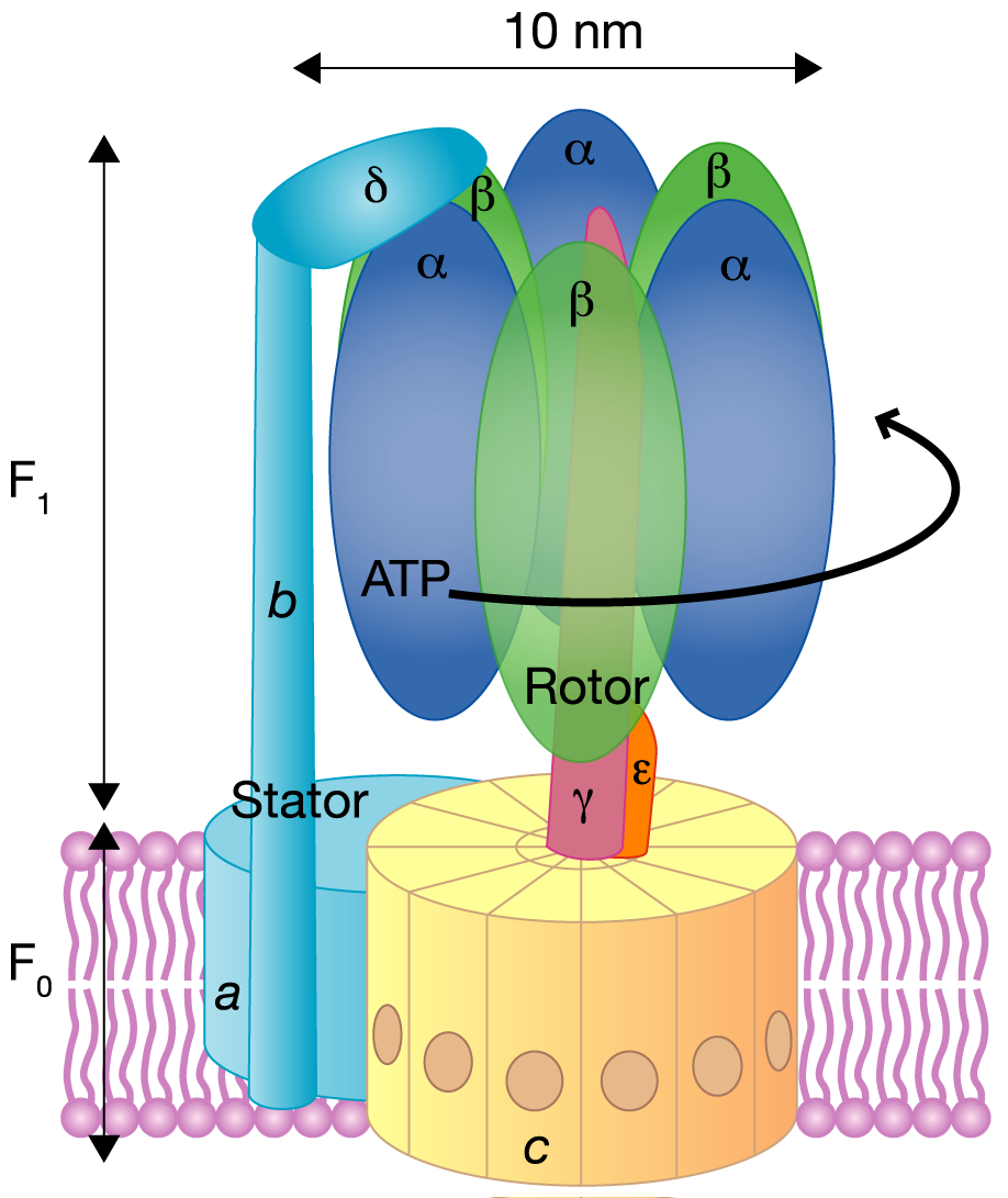
Figure 1: F1-ATPase is a naturally occurring rotating molecular motor. It works as a pump for ions through a membrane. Its driving force is chemical, through the hydrolysis of ATP. Our interest in this molecular motor lies in its environment (in the cytoplasm, subject to fluctuations), its construction (rotational, and through a biological membrane), its physical characteristics (size of the order of 10 nm) and dynamical properties (rotational frequency of the order of 100 Hz).

F1-ATPase is a well-known rotating motor (see Fig. 1 for a diagram). A direct observation of its rotation, driven by the hydrolysis of adenosine triphosphate (ATP), was first reported in Noji ; Yasuda . Later experiments Itoh revealed the direction in which the ATP motor spins. It is about 10 nm in size and typically rotates with a frequency of 100 Hz. The observed rotary torque reaches more than 40 pN nm. The relation between the geometry of the rotating object, specifically its chirality, and its kinetic properties, such as the average motion and friction can be of interest to microbiology. One might also imagine artificial devices inspired by the existing biological examples. Proteins could be used as the building blocks of mechanical devices and artificial biological membranes as means to separate reservoirs and keep them at different temperature. Small moving parts in the area of micro-electronics are also subject to random fluctuations.
Refer to caption
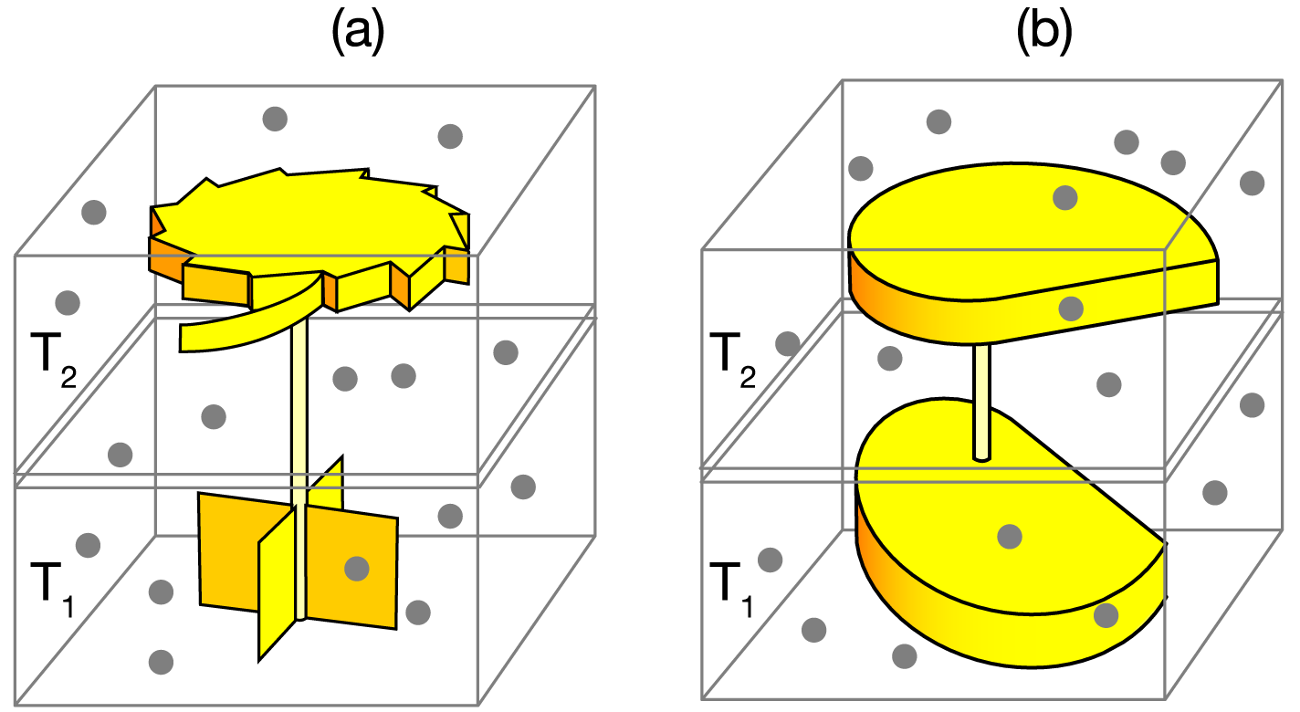
Figure 2: (a) The ratchet and pawl mechanism used by R. Feynman to illustrate the impossibility to extract work from a system in equilibrium. An axle with vanes in it (in the right reservoir ) is bombarded by gas molecules at temperature T1subscript𝑇1T_{1}. The pawl in the left reservoir (surrounded by a gas at temperature T2subscript𝑇2T_{2}) seems to allow only one rotation sense of the ratchet, that is connected with the axle. The fluctuations of the paddle in the right reservoir would then be rectified. Via a comparison of the probability to move forward and backward, Feynman showed in his Lectures on Physics feynman that at temperature equilibrium, T1=T2subscript𝑇1subscript𝑇2T_{1}=T_{2}, no average motion occurs and the device cannot be used to do work, such as to lift a weight. For T1>T2subscript𝑇1subscript𝑇2T_{1}>T_{2} however, average motion does take place and the ratchet works as an engine. Feynman noted that for T1<T2subscript𝑇1subscript𝑇2T_{1}<T_{2}, the ratchet goes backward. Note that the rectification manifested by the device originates from the asymmetry of the ratchet and pawl mechanism. Our model remains close to Feynman’s system, as it can be applied to rotating three-dimensional objects of any shape, while it simplifies the asymmetry requirements to the geometrical properties of the device. (b) A rotating Brownian motor where two parts in isolated thermal reservoirs (temperatures T1subscript𝑇1T_{1} and T2subscript𝑇2T_{2}, particle densities ρ1subscript𝜌1\rho_{1} and ρ2subscript𝜌2\rho_{2}) are connected through the axis of rotation. Collisions with particles in the reservoirs will cause fluctuating rotational movement of the heavier motor, which under appropriate conditions, will propel the motor with a nonzero average angular velocity.

As a side note we remark that the rotational three-dimensional model we will present, can be used to describe the essence of the device R. Feynman presented in his Lectures on Physics feynman [for a sketch of the ratchet and pawl mechanism, see Fig. 2(a)] to illustrate the impossibility of a Maxwell Demon, that would be able to extract work from a system in equilibrium. It was also shown that the same device can lift a weight (do work) at temperature disequilibrium.

These reasons motivate us to study a chiral Brownian motor in detail. The constituting parts of the motor are in different thermal reservoirs. In an analytical analysis we will derive expressions for the kinetic properties of the motor as a function of the external parameters of the system. It will be made clear that temperature equilibrium between the different reservoirs results in zero average motion and hence prohibits the creation of a Maxwell Demon. On the other hand we will demonstrate the importance of the configuration of the building blocks of the motor and their actual shape, as well as their position relative to the rotation axis. Some emphasis is put on finding optimum operation, yielding maximum average angular velocity. The chiral Brownian motor presented in this paper is a precursor for the chiral Brownian refrigerator presented in the next. The exact relationship derived here between the angular velocity and the temperature gradient will be a crucial step in the investigation of the cooling potential.

The concrete model we propose consists of at least two parts, each residing in a thermal reservoir i=1,2,𝑖12i=1,2,\ldots, that are rigidly connected with each other through a rotation axis. Fig. 2(b) shows the construction of two parts in reservoirs of temperature T1subscript𝑇1T_{1} and T2subscript𝑇2T_{2}, and particle densities ρ1subscript𝜌1\rho_{1} and ρ2subscript𝜌2\rho_{2}. We expect that the fluctuations from collisions with particles in the thermal reservoirs will under certain conditions be rectified, resulting is an average rotational motion, clockwise or counterclockwise. As we will show, these conditions are (1) thermal disequilibrium, T1T2subscript𝑇1subscript𝑇2T_{1}\neq T_{2}, and (2) asymmetry (or chirality) through the geometrical shape of the motor parts.

III From fluctuations to the angular velocity

Our analysis is based on an exact calculation of the probability for the motor to change its rotating speed by a certain amount when subject to thermal fluctuations. We will show that an exact solution can be reached when the fluctuations are in the form of collisions of particles of an ideal gas at temperature equilibrium with the surface of the motor. A master equation for the probability density to observe an angular velocity P(ω,t)𝑃𝜔𝑡P(\omega,t) at a certain time t𝑡t can be proposed if the particles are presumed to collide not more than once, and only with the motor. This condition implies that the gas is in the high Knudsen number regime and that the shape of the motor is such that recollisions are impossible. We therefore limit the parts of the motor to convex and closed shapes.

We are interested in the case where the motor, with total mass M𝑀M, has no translational degree of freedom and a single rotational degree of freedom. Parts of the motor reside in different thermal reservoirs but are considered rigidly linked. Choosing the z𝑧z-axis as the axis of rotation, we can write for the angular velocity ω=(0,0,ω)𝜔00𝜔\vec{\omega}=(0,0,\omega). The inertial moment Izsubscript𝐼𝑧I_{z} of the motor with respect to the rotation axis is simply denoted as I𝐼I.

Under these conditions the probability density P(ω,t)𝑃𝜔𝑡P(\omega,t) obeys a master equation,

tP(ω,t)=𝑑ω[W(ω|ω)P(ω,t)W(ω|ω)P(ω,t)],subscript𝑡𝑃𝜔𝑡differential-dsuperscript𝜔delimited-[]𝑊conditional𝜔superscript𝜔𝑃superscript𝜔𝑡𝑊conditionalsuperscript𝜔𝜔𝑃𝜔𝑡\partial_{t}P(\omega,t)=\int d\omega^{\prime}\left[W(\omega|\omega^{\prime})P(\omega^{\prime},t)-W(\omega^{\prime}|\omega)P(\omega,t)\right], (1)

where W(ω|ω)𝑊conditional𝜔superscript𝜔W(\omega|\omega^{\prime}) is the transition probability per unit time for the motor to change its angular velocity from ωsuperscript𝜔\omega^{\prime} to ω𝜔\omega. The solution is based on the van Kampen 1/Ω1Ω1/\Omega-method vankampen . A Taylor expansion of the first term of the integrand in the angular velocity change, υ=ωω𝜐𝜔superscript𝜔\upsilon=\omega-\omega^{\prime}, leads to

tP(ω,t)=n=1(1)nn!(ddω)n{an(ω)P(ω,t)}.subscript𝑡𝑃𝜔𝑡superscriptsubscript𝑛1superscript1𝑛𝑛superscript𝑑𝑑𝜔𝑛subscript𝑎𝑛𝜔𝑃𝜔𝑡\partial_{t}P(\omega,t)=\sum_{n=1}^{\infty}\frac{(-1)^{n}}{n!}\left(\frac{d}{d\omega}\right)^{n}\{a_{n}(\omega)P(\omega,t)\}. (2)

In this expression the so-called jump moments appear, given by

an(ω)=υnW(ω;υ)𝑑υ.subscript𝑎𝑛𝜔superscript𝜐𝑛𝑊𝜔𝜐differential-d𝜐a_{n}(\omega)=\int\upsilon^{n}W(\omega;\upsilon)d\upsilon. (3)

A notation W(ω;υ)=W(ω|ω)𝑊superscript𝜔𝜐𝑊conditional𝜔superscript𝜔W(\omega^{\prime};\upsilon)=W(\omega|\omega^{\prime}) is used. With the time evolution of the probability density known (Eq. 2), it is possible to derive a coupled set of equations for the moments of the angular velocity ωndelimited-⟨⟩superscript𝜔𝑛\langle\omega^{n}\rangle:

tωn=k=1n(nk)ωnkak(ω),subscript𝑡delimited-⟨⟩superscript𝜔𝑛superscriptsubscript𝑘1𝑛binomial𝑛𝑘delimited-⟨⟩superscript𝜔𝑛𝑘subscript𝑎𝑘𝜔\partial_{t}\langle\omega^{n}\rangle=\sum_{k=1}^{n}\binom{n}{k}\langle\omega^{n-k}a_{k}(\omega)\rangle, (4)

with (nk)binomial𝑛𝑘\binom{n}{k} the binomial coefficients. Our strategy is now clear: first find an expression for the transition probability W(ω|ω)𝑊conditional𝜔superscript𝜔W(\omega|\omega^{\prime}), then calculate the jump moments an(ω)subscript𝑎𝑛𝜔a_{n}(\omega), and finally the moments of the angular velocity ωndelimited-⟨⟩superscript𝜔𝑛\langle\omega^{n}\rangle.

However, the coupled set of equations Eq. 4 cannot be solved unless we expand each equation into powers of a small variable, and ignore terms after a certain order. For the expansion variable we will use ε=r0m/I𝜀subscript𝑟0𝑚𝐼\varepsilon=r_{0}\sqrt{m/I}, with r0=I/Msubscript𝑟0𝐼𝑀r_{0}=\sqrt{I/M} the radius of gyration of the motor. We also introduce an effective temperature Teffsubscript𝑇effT_{\text{eff}}, so that to first significant order, in the regime of stationary motion, the average kinetic energy of the motor is given by

12Iω2=12kBTeff.12𝐼delimited-⟨⟩superscript𝜔212subscript𝑘𝐵subscript𝑇eff\frac{1}{2}I\langle\omega^{2}\rangle=\frac{1}{2}k_{B}T_{\text{eff}}. (5)

In the calculation it is convenient to do a transformation to dimensionless variables, by scaling the angular velocity ω𝜔\omega and the jump moments ansubscript𝑎𝑛a_{n} as follows:

ξ𝜉\displaystyle\xi =ωI/kBTeff,absent𝜔𝐼subscript𝑘𝐵subscript𝑇eff\displaystyle=\omega\sqrt{I/k_{B}T_{\text{eff}}},
An(ξ)subscript𝐴𝑛𝜉\displaystyle A_{n}(\xi) =(I/kBTeff)nan(ξ).absentsuperscript𝐼subscript𝑘𝐵subscript𝑇eff𝑛subscript𝑎𝑛𝜉\displaystyle=(\sqrt{I/k_{B}T_{\text{eff}}})^{n}a_{n}(\xi). (6)

Our selfconsistent definition of the effective temperature Teffsubscript𝑇effT_{\text{eff}} then leads to ξ2=1delimited-⟨⟩superscript𝜉21\langle\xi^{2}\rangle=1 for the stationary state to first order in ε𝜀\varepsilon. The set of coupled equations for the moments ξn=ξnP(ξ,t)𝑑ξdelimited-⟨⟩superscript𝜉𝑛superscript𝜉𝑛𝑃𝜉𝑡differential-d𝜉\langle\xi^{n}\rangle=\int\xi^{n}P(\xi,t)d\xi remains

tξn=k=1n(nk)ξnkAk(ξ).subscript𝑡delimited-⟨⟩superscript𝜉𝑛superscriptsubscript𝑘1𝑛binomial𝑛𝑘delimited-⟨⟩superscript𝜉𝑛𝑘subscript𝐴𝑘𝜉\partial_{t}\langle\xi^{n}\rangle=\sum_{k=1}^{n}\binom{n}{k}\langle\xi^{n-k}A_{k}(\xi)\rangle. (7)

IV Two-dimensional model of the motor

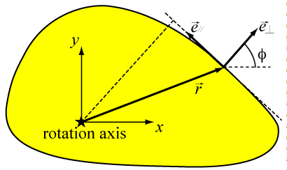
The motor consists of parts with hard surfaces of arbitrary (but convex) shape, each described by their boundary and inner mass distribution. Many of the important features already appear in a simpler two-dimensional system, which we present first. Here the motor consists of two-dimensional shapes, each in two-dimensional reservoirs. We choose a cartesian coordinate system as follows: the z𝑧z-axis coincides with the rotation axis, while the xy𝑥𝑦xy-plane is parallel to the reservoirs. In each reservoir i𝑖i, the shape of the motor (part) is defined by its boundary ri(x,y)subscript𝑟𝑖𝑥𝑦\vec{r}_{i}(x,y), given as a vector with the rotation axis as its origin (see Fig. 3). The perimeter of the boundary is denoted Lisubscript𝐿𝑖L_{i}. Henceforth we will just write r(x,y)𝑟𝑥𝑦\vec{r}(x,y) for ri(x,y)subscript𝑟𝑖𝑥𝑦\vec{r}_{i}(x,y) as no confusion can arise in subsequent expressions.
Refer to caption
Figure 3: In each reservoir, the motor part can be described by the boundary r(x,y)𝑟𝑥𝑦\vec{r}(x,y), where the rotation axis is at the origin of the reference frame. It is convenient to also know explicitly the orientation of the boundary at any point. This is given by the polar angle φ𝜑\varphi of the normal outward vector esubscript𝑒perpendicular-to\vec{e}_{\perp} on the surface at this point. The unit vector esubscript𝑒parallel-to\vec{e}_{\shortparallel} is tangential to the boundary.

It is convenient in the further derivation to explicitly know the inclination of the boundary at r(x,y)𝑟𝑥𝑦\vec{r}(x,y), for which we use the orientation of the normal outward unit vector e=(cosφ,sinφ)subscript𝑒perpendicular-to𝜑𝜑\vec{e}_{\perp}=(\cos\varphi,\sin\varphi) on the boundary, determined by the polar coordinate φ𝜑\varphi from the x𝑥x-axis.

IV.1 Conservation rules

Fluctuations of the angular velocity ω𝜔\omega of motor arise from collisions on the surface with gas particles of mass m𝑚m. Such a collision – presumed instantaneous and perfectly elastic – changes the velocity of the gas particle v=(vx,vy)superscript𝑣subscriptsuperscript𝑣𝑥subscriptsuperscript𝑣𝑦\vec{v^{\prime}}=(v^{\prime}_{x},v^{\prime}_{y}) into v=(vx,vy)𝑣subscript𝑣𝑥subscript𝑣𝑦\vec{v}=(v_{x},v_{y}) after the collision, while the motor changes angular speed from ωsuperscript𝜔\omega^{\prime} to ω𝜔\omega. The inertial moment of the motor about the rotation axis (z𝑧z-axis) is denoted I𝐼I, while its mass is M𝑀M. Conservation of the total energy requires that

12Iω2+12mvx2+12mvy2=12Iω2+12mvx2+12mvy2,12𝐼superscriptsuperscript𝜔212𝑚superscriptsubscriptsuperscript𝑣𝑥212𝑚superscriptsubscriptsuperscript𝑣𝑦212𝐼superscript𝜔212𝑚superscriptsubscript𝑣𝑥212𝑚superscriptsubscript𝑣𝑦2\frac{1}{2}I{\omega^{\prime}}^{2}+\frac{1}{2}m{v^{\prime}_{x}}^{2}+\frac{1}{2}m{v^{\prime}_{y}}^{2}=\frac{1}{2}I\omega^{2}+\frac{1}{2}mv_{x}^{2}+\frac{1}{2}mv_{y}^{2}, (8a)
while conservation of the angular momentum in the z𝑧z-direction yields
m(xvyyvx)+Iω=m(xvyyvx)+Iω.𝑚𝑥subscriptsuperscript𝑣𝑦𝑦subscriptsuperscript𝑣𝑥𝐼superscript𝜔𝑚𝑥subscript𝑣𝑦𝑦subscript𝑣𝑥𝐼𝜔m(xv^{\prime}_{y}-yv^{\prime}_{x})+I\omega^{\prime}=m(xv_{y}-yv_{x})+I\omega. (8b)
Also we suppose the interaction force is short-ranged and central, implying that the tangent component of the momentum of the gas particle on the boundary is conserved. Choosing the tangent unit vector e=(sinφ,cosφ)subscript𝑒parallel-to𝜑𝜑\vec{e}_{\shortparallel}=(-\sin\varphi,\cos\varphi), so that (e,e)subscript𝑒perpendicular-tosubscript𝑒parallel-to(\vec{e}_{\perp},\vec{e}_{\shortparallel}) forms a positive orthonormal base, we write
ve=ve.superscript𝑣subscript𝑒parallel-to𝑣subscript𝑒parallel-to\vec{v^{\prime}}\cdot\vec{e}_{\shortparallel}=\vec{v}\cdot\vec{e}_{\shortparallel}. (8c)

The conservation laws (Eq. 8c) produce a solution for the postcollisional angular velocity ω𝜔\omega,

ω=ω+2(ωy+vx)cosφ2(ωxvy)sinφxsinφycosφ+Im(xsinφycosφ)1,𝜔superscript𝜔2superscript𝜔𝑦subscriptsuperscript𝑣𝑥𝜑2superscript𝜔𝑥subscriptsuperscript𝑣𝑦𝜑𝑥𝜑𝑦𝜑𝐼𝑚superscript𝑥𝜑𝑦𝜑1\omega=\omega^{\prime}+\frac{2(\omega^{\prime}y+v^{\prime}_{x})\cos\varphi-2(\omega^{\prime}x-v^{\prime}_{y})\sin\varphi}{x\sin\varphi-y\cos\varphi+\frac{I}{m}\left(x\sin\varphi-y\cos\varphi\right)^{-1}}, (9)

Introducing

r=re=xsinφ+ycosφ,subscript𝑟parallel-to𝑟subscript𝑒parallel-to𝑥𝜑𝑦𝜑r_{\shortparallel}=\vec{r}\cdot\vec{e}_{\shortparallel}=-x\sin\varphi+y\cos\varphi, (10)

and the precollisional speed of the boundary at position r𝑟\vec{r},

V=ω×r=(ωy,ωx),superscript𝑉superscript𝜔𝑟superscript𝜔𝑦superscript𝜔𝑥\vec{V^{\prime}}=\vec{\omega^{\prime}}\times\vec{r}=(-\omega^{\prime}y,\omega^{\prime}x), (11)

so that we can write

V=Ve=ωycosφ+ωxsinφ,subscriptsuperscript𝑉perpendicular-tosuperscript𝑉subscript𝑒perpendicular-tosuperscript𝜔𝑦𝜑superscript𝜔𝑥𝜑V^{\prime}_{\perp}=\vec{V^{\prime}}\cdot\vec{e}_{\perp}=-\omega^{\prime}y\cos\varphi+\omega^{\prime}x\sin\varphi, (12)

and

ΔV=(Vv)e=(ωy+vx)cosφ+(ωxvy)sinφ,Δsubscriptsuperscript𝑉perpendicular-tosuperscript𝑉superscript𝑣subscript𝑒perpendicular-tosuperscript𝜔𝑦subscriptsuperscript𝑣𝑥𝜑superscript𝜔𝑥subscriptsuperscript𝑣𝑦𝜑\Delta V^{\prime}_{\perp}=(\vec{V^{\prime}}-\vec{v^{\prime}})\cdot\vec{e}_{\perp}=-(\omega^{\prime}y+v^{\prime}_{x})\cos\varphi+(\omega^{\prime}x-v^{\prime}_{y})\sin\varphi, (13)

the transition in ω𝜔\omega can also be written as

ω=ω+2ΔVr+Imr.𝜔superscript𝜔2Δsubscriptsuperscript𝑉perpendicular-tosubscript𝑟parallel-to𝐼𝑚subscript𝑟parallel-to\omega=\omega^{\prime}+2\frac{\Delta V^{\prime}_{\perp}}{r_{\shortparallel}+\frac{I}{mr_{\shortparallel}}}. (14)

IV.2 Transition probability

Next, we set out to find the crucial transition probability W(ω|ω)𝑊conditional𝜔superscript𝜔W(\omega|\omega^{\prime}) for the motor to change its angular velocity from ωsuperscript𝜔\omega^{\prime} to ω𝜔\omega in a unit of time. Every reservoir i𝑖i contains a gas with particle density ρisubscript𝜌𝑖\rho_{i} and velocity distribution ϕisubscriptitalic-ϕ𝑖\phi_{i}. The contribution dWi𝑑subscript𝑊𝑖dW_{i} to the total transition probability W(ω|ω)𝑊conditional𝜔superscript𝜔W(\omega|\omega^{\prime}) from all possible collisions of particles in gas i𝑖i in a time interval dt𝑑𝑡dt on a boundary section of length dli𝑑subscript𝑙𝑖dl_{i}, at position r(x,y)𝑟𝑥𝑦\vec{r}(x,y) and with orientation φ𝜑\varphi, can be expressed as

dWi(ω|ω)=dli+𝑑vx+𝑑vy×H[(Vv)e]|(Vv)e|ρiϕi(vx,vy)×δ[ωω2(ωy+vx)cosφ2(ωxvy)sinφxsinφycosφ+Im(xsinφycosφ)1],𝑑subscript𝑊𝑖conditional𝜔superscript𝜔𝑑subscript𝑙𝑖superscriptsubscriptdifferential-dsubscriptsuperscript𝑣𝑥superscriptsubscriptdifferential-dsubscriptsuperscript𝑣𝑦𝐻delimited-[]superscript𝑉superscript𝑣subscript𝑒perpendicular-tosuperscript𝑉superscript𝑣subscript𝑒perpendicular-tosubscript𝜌𝑖subscriptitalic-ϕ𝑖subscriptsuperscript𝑣𝑥subscriptsuperscript𝑣𝑦𝛿delimited-[]𝜔superscript𝜔2superscript𝜔𝑦subscriptsuperscript𝑣𝑥𝜑2superscript𝜔𝑥subscriptsuperscript𝑣𝑦𝜑𝑥𝜑𝑦𝜑𝐼𝑚superscript𝑥𝜑𝑦𝜑1dW_{i}(\omega|\omega^{\prime})=dl_{i}\int_{-\infty}^{+\infty}\negthickspace\negthickspace dv^{\prime}_{x}\int_{-\infty}^{+\infty}\negthickspace\negthickspace dv^{\prime}_{y}\\ \times H[(\vec{V^{\prime}}-\vec{v^{\prime}})\cdot\vec{e}_{\perp}]|(\vec{V^{\prime}}-\vec{v^{\prime}})\cdot\vec{e}_{\perp}|\rho_{i}\phi_{i}(v^{\prime}_{x},v^{\prime}_{y})\\ \times\delta\left[\omega-\omega^{\prime}-\frac{2(\omega^{\prime}y+v^{\prime}_{x})\cos\varphi-2(\omega^{\prime}x-v^{\prime}_{y})\sin\varphi}{x\sin\varphi-y\cos\varphi+\frac{I}{m}\left(x\sin\varphi-y\cos\varphi\right)^{-1}}\right], (15)

with H𝐻H the Heaviside step function and δ𝛿\delta Dirac’s distribution. We multiplied the particle density ρisubscript𝜌𝑖\rho_{i} with the volume of the gas that is passed by the boundary element dli𝑑subscript𝑙𝑖dl_{i} in a time unit, considering only those gas particles that comply with the collision rules. This can be written in short form as

dWi(ω|ω)=dli+𝑑vx+𝑑vyH[ΔV]|ΔV|×ρiϕi(vx,vy)δ[ωω2ΔVr+Imr].𝑑subscript𝑊𝑖conditional𝜔superscript𝜔𝑑subscript𝑙𝑖superscriptsubscriptdifferential-dsubscriptsuperscript𝑣𝑥superscriptsubscriptdifferential-dsubscriptsuperscript𝑣𝑦𝐻delimited-[]Δsubscriptsuperscript𝑉perpendicular-toΔsubscriptsuperscript𝑉perpendicular-tosubscript𝜌𝑖subscriptitalic-ϕ𝑖subscriptsuperscript𝑣𝑥subscriptsuperscript𝑣𝑦𝛿delimited-[]𝜔superscript𝜔2Δsubscriptsuperscript𝑉perpendicular-tosubscript𝑟parallel-to𝐼𝑚subscript𝑟parallel-todW_{i}(\omega|\omega^{\prime})=dl_{i}\int_{-\infty}^{+\infty}\negthickspace\negthickspace dv^{\prime}_{x}\int_{-\infty}^{+\infty}\negthickspace\negthickspace dv^{\prime}_{y}H[\Delta V^{\prime}_{\perp}]|\Delta V^{\prime}_{\perp}|\\ \times\rho_{i}\phi_{i}(v^{\prime}_{x},v^{\prime}_{y})\delta\left[\omega-\omega^{\prime}-2\frac{\Delta V^{\prime}_{\perp}}{r_{\shortparallel}+\frac{I}{mr_{\shortparallel}}}\right]. (16)

The total transition probability is then found by integrating over all boundary elements dli𝑑subscript𝑙𝑖dl_{i} and summing over all reservoirs:

W(ω|ω)=iboundary𝑑Wi(ω|ω).𝑊conditional𝜔superscript𝜔subscript𝑖subscriptcontour-integralboundarydifferential-dsubscript𝑊𝑖conditional𝜔superscript𝜔W(\omega|\omega^{\prime})=\sum_{i}\oint_{\text{boundary}}\negthickspace\negthickspace\negthickspace\negthickspace\negthickspace\negthickspace\negthickspace\negthickspace\negthickspace\negthickspace dW_{i}(\omega|\omega^{\prime}). (17)

Henceforth we will simply write contour-integral\oint when we imply the line integral over all boundary elements.

For a Maxwellian velocity distribution at temperature Tisubscript𝑇𝑖T_{i},

ϕi(vx,vy)=m2πkBTiexp(m(vx2+vy22kBTi),\phi_{i}(v_{x},v_{y})=\frac{m}{2\pi k_{B}T_{i}}\exp\left(\frac{-m(v_{x}^{2}+v_{y}^{2}}{2k_{B}T_{i}}\right), (18)

the integrals over the speed of the colliding particles can be performed explicitly, resulting in

W(ω|ω)=14i𝑑liρim2πkBTi×(r+Imr)2H[(ωω)r]|ωω|×exp[m2kBTi((r+Imr)ωω2rω)2].𝑊conditional𝜔superscript𝜔14subscript𝑖contour-integraldifferential-dsubscript𝑙𝑖subscript𝜌𝑖𝑚2𝜋subscript𝑘𝐵subscript𝑇𝑖superscriptsubscript𝑟parallel-to𝐼𝑚subscript𝑟parallel-to2𝐻delimited-[]𝜔superscript𝜔subscript𝑟parallel-to𝜔superscript𝜔𝑚2subscript𝑘𝐵subscript𝑇𝑖superscriptsubscript𝑟parallel-to𝐼𝑚subscript𝑟parallel-tosuperscript𝜔𝜔2subscript𝑟parallel-tosuperscript𝜔2W(\omega|\omega^{\prime})=\frac{1}{4}\sum_{i}\oint dl_{i}\rho_{i}\sqrt{\frac{m}{2\pi k_{B}T_{i}}}\\ \times(r_{\shortparallel}+\frac{I}{mr_{\shortparallel}})^{2}H[(\omega-\omega^{\prime})r_{\shortparallel}]|\omega-\omega^{\prime}|\\ \times\exp\left[-\frac{m}{2k_{B}T_{i}}\left((r_{\shortparallel}+\frac{I}{mr_{\shortparallel}})\frac{\omega^{\prime}-\omega}{2}-r_{\shortparallel}\omega^{\prime}\right)^{2}\right]. (19)

IV.3 Moments of the angular velocity

Now that we have obtained an exact expression for the transition probability W(ω|ω)𝑊conditional𝜔superscript𝜔W(\omega|\omega^{\prime}), we turn our attention to the jump moments,

an(ω)=υnW(ω;υ)𝑑υ,subscript𝑎𝑛𝜔superscript𝜐𝑛𝑊𝜔𝜐differential-d𝜐a_{n}(\omega)=\int\upsilon^{n}W(\omega;\upsilon)d\upsilon, (20)

and then the moments of the angular velocity. Careful consideration of the sign of r+I/mrsubscript𝑟parallel-to𝐼𝑚subscript𝑟parallel-tor_{\shortparallel}+I/mr_{\shortparallel} in

W(ω;υ)=14iρim2πkBTi×(H[υ]r0𝑑li+H[υ]r<0𝑑li)|υ|(r+Imr)2×exp[m2kBTi((r+Imr)υ2+rω)2],𝑊𝜔𝜐14subscript𝑖subscript𝜌𝑖𝑚2𝜋subscript𝑘𝐵subscript𝑇𝑖𝐻delimited-[]𝜐subscriptsubscript𝑟parallel-to0differential-dsubscript𝑙𝑖𝐻delimited-[]𝜐subscriptsubscript𝑟parallel-to0differential-dsubscript𝑙𝑖𝜐superscriptsubscript𝑟parallel-to𝐼𝑚subscript𝑟parallel-to2𝑚2subscript𝑘𝐵subscript𝑇𝑖superscriptsubscript𝑟parallel-to𝐼𝑚subscript𝑟parallel-to𝜐2subscript𝑟parallel-to𝜔2W(\omega;\upsilon)=\frac{1}{4}\sum_{i}\rho_{i}\sqrt{\frac{m}{2\pi k_{B}T_{i}}}\\ \times\left(H[\upsilon]\int_{r_{\shortparallel}\geq 0}dl_{i}+H[-\upsilon]\int_{r_{\shortparallel}<0}dl_{i}\right)|\upsilon|(r_{\shortparallel}+\frac{I}{mr_{\shortparallel}})^{2}\\ \times\exp\left[-\frac{m}{2k_{B}T_{i}}\left((r_{\shortparallel}+\frac{I}{mr_{\shortparallel}})\frac{\upsilon}{2}+r_{\shortparallel}\omega\right)^{2}\right], (21)

where υ=ωω𝜐𝜔superscript𝜔\upsilon=\omega-\omega^{\prime} is the change in angular velocity, leads to an exact expression for the jump moments. In terms of parabolic cylinder functions, Dn(z)=(exp[z2/4]/Γ[n])0exp[zxx2/2]xn1𝑑xsubscriptD𝑛𝑧superscript𝑧24Γdelimited-[]𝑛superscriptsubscript0𝑧𝑥superscript𝑥22superscript𝑥𝑛1differential-d𝑥\operatorname{D}_{n}(z)=\left(\exp[-z^{2}/4]/\Gamma[-n]\right)\int_{0}^{\infty}\exp[-zx-x^{2}/2]x^{-n-1}dx (for n<0𝑛0n<0) the results are

an(ω)=2n2πΓ[n+2]iρi(mkBTi)n+12×dliρi(r+Imr)n×exp[m4kBTir2ω2]Dn2[mkBTirω].subscript𝑎𝑛𝜔superscript2𝑛2𝜋Γdelimited-[]𝑛2subscript𝑖subscript𝜌𝑖superscript𝑚subscript𝑘𝐵subscript𝑇𝑖𝑛12contour-integral𝑑subscript𝑙𝑖subscript𝜌𝑖superscriptsubscript𝑟parallel-to𝐼𝑚subscript𝑟parallel-to𝑛𝑚4subscript𝑘𝐵subscript𝑇𝑖superscriptsubscript𝑟parallel-to2superscript𝜔2subscriptD𝑛2𝑚subscript𝑘𝐵subscript𝑇𝑖subscript𝑟parallel-to𝜔a_{n}(\omega)=\frac{2^{n}}{\sqrt{2\pi}}\Gamma[n+2]\sum_{i}\rho_{i}\left(\frac{m}{k_{B}T_{i}}\right)^{-\frac{n+1}{2}}\\ \times\oint dl_{i}\rho_{i}\left(r_{\shortparallel}+\frac{I}{mr_{\shortparallel}}\right)^{-n}\\ \times\exp\left[-\frac{m}{4k_{B}T_{i}}r_{\shortparallel}^{2}\omega^{2}\right]\operatorname{D}_{-n-2}\left[\sqrt{\frac{m}{k_{B}T_{i}}}r_{\shortparallel}\omega\right]. (22)

Rescaling the jump moments using dimensionless variables ξ=ωI/kBTeff𝜉𝜔𝐼subscript𝑘𝐵subscript𝑇eff\xi=\omega\sqrt{I/k_{B}T_{\text{eff}}} and ε=r0m/I𝜀subscript𝑟0𝑚𝐼\varepsilon=r_{0}\sqrt{m/I}, where r02=I/Msuperscriptsubscript𝑟02𝐼𝑀r_{0}^{2}=I/M, leads to

An(ξ)=(I/kBTeff)nan(ξ)=23n12πiρikBTim(TiTeff)n/2×dli(εr/r01+ε2(r/r0)2)n×exp[ε22TeffTi(r/r0)2ξ2]×(Γ[n+22]Φ[n+22;12;ε22TeffTi(r/r0)2ξ2]2εTeffTirr0ξΓ[n+32]×Φ[n+32;32;ε22TeffTi(r/r0)2ξ2]).subscript𝐴𝑛𝜉superscript𝐼subscript𝑘𝐵subscript𝑇eff𝑛subscript𝑎𝑛𝜉superscript23𝑛12𝜋subscript𝑖subscript𝜌𝑖subscript𝑘𝐵subscript𝑇𝑖𝑚superscriptsubscript𝑇𝑖subscript𝑇eff𝑛2contour-integral𝑑subscript𝑙𝑖superscript𝜀subscript𝑟parallel-tosubscript𝑟01superscript𝜀2superscriptsubscript𝑟parallel-tosubscript𝑟02𝑛superscript𝜀22subscript𝑇effsubscript𝑇𝑖superscriptsubscript𝑟parallel-tosubscript𝑟02superscript𝜉2Γdelimited-[]𝑛22Φ𝑛2212superscript𝜀22subscript𝑇effsubscript𝑇𝑖superscriptsubscript𝑟parallel-tosubscript𝑟02superscript𝜉22𝜀subscript𝑇effsubscript𝑇𝑖subscript𝑟parallel-tosubscript𝑟0𝜉Γdelimited-[]𝑛32Φ𝑛3232superscript𝜀22subscript𝑇effsubscript𝑇𝑖superscriptsubscript𝑟parallel-tosubscript𝑟02superscript𝜉2A_{n}(\xi)=(\sqrt{I/k_{B}T_{\text{eff}}})^{n}a_{n}(\xi)\\ =\frac{2^{\frac{3n-1}{2}}}{\sqrt{\pi}}\sum_{i}\rho_{i}\sqrt{\frac{k_{B}T_{i}}{m}}\left(\frac{T_{i}}{T_{\text{eff}}}\right)^{n/2}\\ \times\oint dl_{i}\left(\frac{\varepsilon r_{\shortparallel}/r_{0}}{1+\varepsilon^{2}(r_{\shortparallel}/r_{0})^{2}}\right)^{n}\\ \times\exp\left[-\frac{\varepsilon^{2}}{2}\frac{T_{\text{eff}}}{T_{i}}(r_{\shortparallel}/r_{0})^{2}\xi^{2}\right]\\ \times\Biggl{(}\Gamma\left[\frac{n+2}{2}\right]\Phi\left[\frac{n+2}{2};\frac{1}{2};\frac{\varepsilon^{2}}{2}\frac{T_{\text{eff}}}{T_{i}}(r_{\shortparallel}/r_{0})^{2}\xi^{2}\right]\\ -\sqrt{2}\varepsilon\sqrt{\frac{T_{\text{eff}}}{T_{i}}}\frac{r_{\shortparallel}}{r_{0}}\xi\;\Gamma\left[\frac{n+3}{2}\right]\\ \times\Phi\left[\frac{n+3}{2};\frac{3}{2};\frac{\varepsilon^{2}}{2}\frac{T_{\text{eff}}}{T_{i}}(r_{\shortparallel}/r_{0})^{2}\xi^{2}\right]\Biggr{)}. (23)

Here ΦΦ\Phi represents Kummer’s function gradshteyn .

We can express both the exponential function and Kummer’s function in a power series,

exp[z]=1+z1!+z22!+z33!+,𝑧1𝑧1superscript𝑧22superscript𝑧33\exp[z]=1+\frac{z}{1!}+\frac{z^{2}}{2!}+\frac{z^{3}}{3!}+\cdots, (24)
Φ[α;γ;z]=1F1[α;γ;z]=1+αγz1!+α(α+1)γ(γ+1)z22!+α(α+1)(α+2)γ(γ+1)(γ+2)z33!+,subscript1Φ𝛼𝛾𝑧subscript𝐹1𝛼𝛾𝑧1𝛼𝛾𝑧1𝛼𝛼1𝛾𝛾1superscript𝑧22𝛼𝛼1𝛼2𝛾𝛾1𝛾2superscript𝑧33\Phi[\alpha;\gamma;z]=\;_{1}F_{1}[\alpha;\gamma;z]=1+\frac{\alpha}{\gamma}\frac{z}{1!}+\frac{\alpha(\alpha+1)}{\gamma(\gamma+1)}\frac{z^{2}}{2!}\\ +\frac{\alpha(\alpha+1)(\alpha+2)}{\gamma(\gamma+1)(\gamma+2)}\frac{z^{3}}{3!}+\cdots, (25)

Considering that the parameter ε=m/M𝜀𝑚𝑀\varepsilon=\sqrt{m/M} is small for gas particles much lighter than the motor, we arrive at a series expansion for the jump moments in ε𝜀\varepsilon. We substitute this expansion in the set of equations (Eq. 23) coupling the jump moments An(ξ)subscript𝐴𝑛𝜉A_{n}(\xi) with the moments of the angular velocity ξndelimited-⟨⟩superscript𝜉𝑛\langle\xi^{n}\rangle. For n=1𝑛1n=1, with τ=ε2t𝜏superscript𝜀2𝑡\tau=\varepsilon^{2}t, this results in

τξsubscript𝜏delimited-⟨⟩𝜉\displaystyle\partial_{\tau}\langle\xi\rangle =ε2A1(ξ)=iρikBTimabsentsuperscript𝜀2delimited-⟨⟩subscript𝐴1𝜉subscript𝑖subscript𝜌𝑖subscript𝑘𝐵subscript𝑇𝑖𝑚\displaystyle=\varepsilon^{-2}\langle A_{1}(\xi)\rangle=\sum_{i}\rho_{i}\sqrt{\frac{k_{B}T_{i}}{m}}
×[\displaystyle\times\biggl{[} ε1TiTeff𝑑li(rr0)22πξ𝑑li(rr0)2superscript𝜀1subscript𝑇𝑖subscript𝑇effcontour-integraldifferential-dsubscript𝑙𝑖subscript𝑟parallel-tosubscript𝑟022𝜋delimited-⟨⟩𝜉contour-integraldifferential-dsubscript𝑙𝑖superscriptsubscript𝑟parallel-tosubscript𝑟02\displaystyle\varepsilon^{-1}\sqrt{\frac{T_{i}}{T_{\text{eff}}}}\oint dl_{i}\left(\frac{r_{\shortparallel}}{r_{0}}\right)-2\sqrt{\frac{2}{\pi}}\langle\xi\rangle\oint dl_{i}\left(\frac{r_{\shortparallel}}{r_{0}}\right)^{2}
+\displaystyle+ ε(TeffTiξ2TiTeff)𝑑li(rr0)3𝜀subscript𝑇effsubscript𝑇𝑖delimited-⟨⟩superscript𝜉2subscript𝑇𝑖subscript𝑇effcontour-integraldifferential-dsubscript𝑙𝑖superscriptsubscript𝑟parallel-tosubscript𝑟03\displaystyle\varepsilon\left(\sqrt{\frac{T_{\text{eff}}}{T_{i}}}\langle\xi^{2}\rangle-\sqrt{\frac{T_{i}}{T_{\text{eff}}}}\right)\oint dl_{i}\left(\frac{r_{\shortparallel}}{r_{0}}\right)^{3}
+\displaystyle+ ε232π(6ξTeffTiξ3)𝑑li(rr0)4superscript𝜀232𝜋6delimited-⟨⟩𝜉subscript𝑇effsubscript𝑇𝑖delimited-⟨⟩superscript𝜉3contour-integraldifferential-dsubscript𝑙𝑖superscriptsubscript𝑟parallel-tosubscript𝑟04\displaystyle\frac{\varepsilon^{2}}{3}\sqrt{\frac{2}{\pi}}\left(6\langle\xi\rangle-\frac{T_{\text{eff}}}{T_{i}}\langle\xi^{3}\rangle\right)\oint dl_{i}\left(\frac{r_{\shortparallel}}{r_{0}}\right)^{4}
+\displaystyle+ ε3(TiTeffTeffTiξ2)dli(rr0)5]+O(ε4).\displaystyle\varepsilon^{3}\left(\sqrt{\frac{T_{i}}{T_{\text{eff}}}}-\sqrt{\frac{T_{\text{eff}}}{T_{i}}}\langle\xi^{2}\rangle\right)\oint dl_{i}\left(\frac{r_{\shortparallel}}{r_{0}}\right)^{5}\biggr{]}+O(\varepsilon^{4}). (26)

The term in ε1superscript𝜀1\varepsilon^{-1} disappears because

𝑑lir=dlir=Ai(×r)ez𝑑Ai=0.contour-integraldifferential-dsubscript𝑙𝑖subscript𝑟parallel-tocontour-integral𝑑subscript𝑙𝑖𝑟subscriptsubscript𝐴𝑖𝑟subscript𝑒𝑧differential-dsubscript𝐴𝑖0\oint dl_{i}r_{\shortparallel}=\oint\vec{dl_{i}}\cdot\vec{r}=\int_{A_{i}}(\nabla\times\vec{r})\cdot\vec{e_{z}}dA_{i}=0. (27)

Similarly for n=2𝑛2n=2,

τξ2subscript𝜏delimited-⟨⟩superscript𝜉2\displaystyle\partial_{\tau}\langle\xi^{2}\rangle =iρikBTimabsentsubscript𝑖subscript𝜌𝑖subscript𝑘𝐵subscript𝑇𝑖𝑚\displaystyle=\sum_{i}\rho_{i}\sqrt{\frac{k_{B}T_{i}}{m}}
×[\displaystyle\times\biggl{[}- 42π(TiTeff+ξ2)𝑑li(rr0)242𝜋subscript𝑇𝑖subscript𝑇effdelimited-⟨⟩superscript𝜉2contour-integraldifferential-dsubscript𝑙𝑖superscriptsubscript𝑟parallel-tosubscript𝑟02\displaystyle 4\sqrt{\frac{2}{\pi}}\left(-\frac{T_{i}}{T_{\text{eff}}}+\langle\xi^{2}\rangle\right)\oint dl_{i}\left(\frac{r_{\shortparallel}}{r_{0}}\right)^{2}
22\displaystyle-2 ε(4TiTeffξTeffTiξ3)𝑑li(rr0)3𝜀4subscript𝑇𝑖subscript𝑇effdelimited-⟨⟩𝜉subscript𝑇effsubscript𝑇𝑖delimited-⟨⟩superscript𝜉3contour-integraldifferential-dsubscript𝑙𝑖superscriptsubscript𝑟parallel-tosubscript𝑟03\displaystyle\varepsilon\left(4\sqrt{\frac{T_{i}}{T_{\text{eff}}}}\langle\xi\rangle-\sqrt{\frac{T_{\text{eff}}}{T_{i}}}\langle\xi^{3}\rangle\right)\oint dl_{i}\left(\frac{r_{\shortparallel}}{r_{0}}\right)^{3}
+22\displaystyle+2 ε22π(4TiTeff+5ξ213TeffTiξ4)𝑑li(rr0)4superscript𝜀22𝜋4subscript𝑇𝑖subscript𝑇eff5delimited-⟨⟩superscript𝜉213subscript𝑇effsubscript𝑇𝑖delimited-⟨⟩superscript𝜉4contour-integraldifferential-dsubscript𝑙𝑖superscriptsubscript𝑟parallel-tosubscript𝑟04\displaystyle\varepsilon^{2}\sqrt{\frac{2}{\pi}}\left(-4\frac{T_{i}}{T_{\text{eff}}}+5\langle\xi^{2}\rangle-\frac{1}{3}\frac{T_{\text{eff}}}{T_{i}}\langle\xi^{4}\rangle\right)\oint dl_{i}\left(\frac{r_{\shortparallel}}{r_{0}}\right)^{4}
+22\displaystyle+2 ε3(7TiTeffξ2TeffTiξ3)dli(rr0)5]\displaystyle\varepsilon^{3}\left(7\sqrt{\frac{T_{i}}{T_{\text{eff}}}}\langle\xi\rangle-2\sqrt{\frac{T_{\text{eff}}}{T_{i}}}\langle\xi^{3}\rangle\right)\oint dl_{i}\left(\frac{r_{\shortparallel}}{r_{0}}\right)^{5}\biggr{]}
+O(\displaystyle+O( ε4).\displaystyle\varepsilon^{4}). (28)

To lowest order in ε𝜀\varepsilon we can extract from Eq. (26) a linear relaxation law for rotational movement, Itω=τf𝐼subscript𝑡delimited-⟨⟩𝜔subscript𝜏𝑓I\partial_{t}\langle\omega\rangle=\tau_{f}, describing a net frictional torque τfsubscript𝜏𝑓\tau_{f} exerted on the motor as a result of all collisions .With τf=γωsubscript𝜏𝑓𝛾delimited-⟨⟩𝜔\tau_{f}=-\gamma\langle\omega\rangle and γ=iγi𝛾subscript𝑖subscript𝛾𝑖\gamma=\sum_{i}\gamma_{i} we derive a microscopic expression for the friction coefficient γisubscript𝛾𝑖\gamma_{i} of each part of the object:

γi=4ρikBTim2π𝑑lir2.subscript𝛾𝑖4subscript𝜌𝑖subscript𝑘𝐵subscript𝑇𝑖𝑚2𝜋contour-integraldifferential-dsubscript𝑙𝑖superscriptsubscript𝑟parallel-to2\gamma_{i}=4\rho_{i}\sqrt{\frac{k_{B}T_{i}m}{2\pi}}\oint dl_{i}r_{\shortparallel}^{2}. (29)

To order ε2superscript𝜀2\varepsilon^{2} the average angular velocity in a stationary state appears from Eq. (26) as

ωdelimited-⟨⟩𝜔\displaystyle\langle\omega\rangle =2πkBm4Iiρi(TeffTi)𝑑lir3iρiTi𝑑lir2absent2𝜋subscript𝑘𝐵𝑚4𝐼subscript𝑖subscript𝜌𝑖subscript𝑇effsubscript𝑇𝑖contour-integraldifferential-dsubscript𝑙𝑖superscriptsubscript𝑟parallel-to3subscript𝑖subscript𝜌𝑖subscript𝑇𝑖contour-integraldifferential-dsubscript𝑙𝑖superscriptsubscript𝑟parallel-to2\displaystyle=\frac{\sqrt{2\pi k_{B}m}}{4I}\frac{\sum_{i}\rho_{i}(T_{\text{eff}}-T_{i})\oint dl_{i}r_{\shortparallel}^{3}}{\sum_{i}\rho_{i}\sqrt{T_{i}}\oint dl_{i}r_{\shortparallel}^{2}}
=kBmγIiρi(TeffTi)𝑑lir3,absentsubscript𝑘𝐵𝑚𝛾𝐼subscript𝑖subscript𝜌𝑖subscript𝑇effsubscript𝑇𝑖contour-integraldifferential-dsubscript𝑙𝑖superscriptsubscript𝑟parallel-to3\displaystyle=\frac{k_{B}m}{\gamma I}\sum_{i}\rho_{i}(T_{\text{eff}}-T_{i})\oint dl_{i}r_{\shortparallel}^{3}, (30)

with second moment,

ω2=kBTeffI,delimited-⟨⟩superscript𝜔2subscript𝑘𝐵subscript𝑇eff𝐼\langle\omega^{2}\rangle=\frac{k_{B}T_{\text{eff}}}{I}, (31)

while the effective temperature is found according to its definition,

Teff=(iγiTi)/(iγi).subscript𝑇effsubscript𝑖subscript𝛾𝑖subscript𝑇𝑖subscript𝑖subscript𝛾𝑖T_{\text{eff}}=(\sum_{i}{\gamma_{i}T_{i}})/(\sum_{i}{\gamma_{i}}). (32)

Using higher order terms in the expansions for ξndelimited-⟨⟩superscript𝜉𝑛\langle\xi^{n}\rangle results in correction terms to the expressions for ωdelimited-⟨⟩𝜔\langle\omega\rangle and ω2delimited-⟨⟩superscript𝜔2\langle\omega^{2}\rangle. The second terms are in both a factor m/M𝑚𝑀m/M smaller than the first terms.

V Three-dimensional model of the motor

The results of a fully three-dimensional analysis are very similar to those derived in the previous two-dimensional case. We will clarify the key differences here.
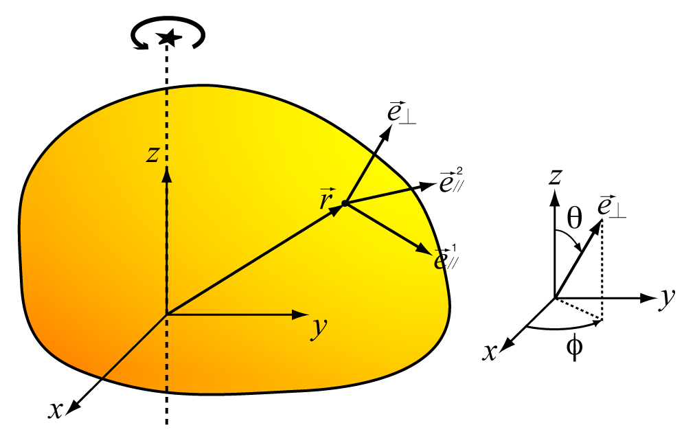
Refer to caption
Figure 4: In each reservoir, the motor part can be described by the boundary r(x,y)𝑟𝑥𝑦\vec{r}(x,y), where the rotation axis is at the origin of the reference frame. It is convenient to also know explicitly the orientation of the boundary at any point. This is given by the polar angle φ𝜑\varphi of the normal outward vector esubscript𝑒perpendicular-to\vec{e}_{\perp} on the surface at this point. The unit vector esubscript𝑒parallel-to\vec{e}_{\shortparallel} is tangential to the boundary.

The motor parts are now determined by their surface Sisubscript𝑆𝑖S_{i} (i𝑖i is the reservoir in which the part resides), to be described by a vector r(x,y,z)𝑟𝑥𝑦𝑧\vec{r}(x,y,z) from the origin. Again we choose the rotation axis to be along the the z𝑧z-axis. The orientation of the surface at a certain location (x,y,z)𝑥𝑦𝑧(x,y,z) is uniquely determined by the normal outward unit vector, e=(sinθcosφ,sinθsinφ,cosθ)subscript𝑒perpendicular-to𝜃𝜑𝜃𝜑𝜃\vec{e}_{\perp}=(\sin\theta\cos\varphi,\sin\theta\sin\varphi,\cos\theta), described by two angles θ𝜃\theta and φ𝜑\varphi, polar and azimuthal angles in a spherical coordinate system.

The assumption that there is only a central force during an interaction with a gas particle, entails that there is conservation of momentum of a gas particle along any tangential direction. So for the speed of the gas particle before ( v=(vx,vy,vz)superscript𝑣subscriptsuperscript𝑣𝑥subscriptsuperscript𝑣𝑦subscriptsuperscript𝑣𝑧\vec{v^{\prime}}=(v^{\prime}_{x},v^{\prime}_{y},v^{\prime}_{z})) and after (v=(vx,vy,vz)𝑣subscript𝑣𝑥subscript𝑣𝑦subscript𝑣𝑧\vec{v}=(v_{x},v_{y},v_{z})) the collision, we can write this condition formally as

vek,=vek,,k=1,2,formulae-sequencesuperscript𝑣subscript𝑒𝑘parallel-to𝑣subscript𝑒𝑘parallel-to𝑘12\vec{v^{\prime}}\cdot\vec{e}_{k,\shortparallel}=\vec{v}\cdot\vec{e}_{k,\shortparallel},\quad k=1,2, (33)

where e1,subscript𝑒1parallel-to\vec{e}_{1,\shortparallel} and e2,subscript𝑒2parallel-to\vec{e}_{2,\shortparallel} are two distinct unit vectors perpendicular to esubscript𝑒perpendicular-to\vec{e}_{\perp}. It is convenient to use e1,=(sinφ,cosφ,0)subscript𝑒1parallel-to𝜑𝜑0\vec{e}_{1,\shortparallel}=(-\sin\varphi,\cos\varphi,0) and e2,=(cosθcosφ,cosθsinφ,sinθ)subscript𝑒2parallel-to𝜃𝜑𝜃𝜑𝜃\vec{e}_{2,\shortparallel}=(\cos\theta\cos\varphi,\cos\theta\sin\varphi,-\sin\theta). Together with conservation of total energy and angular momentum in the z𝑧z-direction (the expressions are the same as in the two-dimensional analysis) we find a relation for the change of angular velocity induced by one collision:

ω=ω+2(Vv)er+Imr.𝜔superscript𝜔2superscript𝑉superscript𝑣subscript𝑒perpendicular-tosubscript𝑟parallel-to𝐼𝑚subscript𝑟parallel-to\omega=\omega^{\prime}+2\frac{(\vec{V^{\prime}}-\vec{v^{\prime}})\cdot\vec{e}_{\perp}}{r_{\shortparallel}+\frac{I}{mr_{\shortparallel}}}. (34)

(Vv)esuperscript𝑉superscript𝑣subscript𝑒perpendicular-to(\vec{V^{\prime}}-\vec{v^{\prime}})\cdot\vec{e}_{\perp} is the component of the velocity difference between motor and gas particle perpendicular to the surface at the place of impact. rsubscript𝑟parallel-tor_{\shortparallel} is now defined as

r=xsinθsinφ+ysinθcosφ=sinθre1,.subscript𝑟parallel-to𝑥𝜃𝜑𝑦𝜃𝜑𝜃𝑟subscript𝑒1parallel-tor_{\shortparallel}=-x\sin\theta\sin\varphi+y\sin\theta\cos\varphi=\sin\theta\>\vec{r}\cdot\vec{e}_{1,\shortparallel}. (35)

rsubscript𝑟parallel-tor_{\shortparallel} is zero in locations where the surface is perpendicular to r𝑟\vec{r}, these coincide with zero momentum transfer. Maximal momentum transfer and rsubscript𝑟parallel-tor_{\shortparallel} occurs when the tangential plane to the surface at this location crosses the rotation axis.

The transition probability dW(ω|ω)𝑑𝑊conditional𝜔superscript𝜔dW(\omega|\omega^{\prime}) caused by all possible collisions with a surface element dSi𝑑subscript𝑆𝑖dS_{i} of the motor, is then found by integrating over all velocities that obey the collision rules,

dWi(ω|ω)=dSi+𝑑vx+𝑑vy+𝑑vz×H[(Vv)e]|(Vv)e|×ρiϕi(vx,vy,vz)δ[ωω2(Vv)er+Imr].𝑑subscript𝑊𝑖conditional𝜔superscript𝜔𝑑subscript𝑆𝑖superscriptsubscriptdifferential-dsubscriptsuperscript𝑣𝑥superscriptsubscriptdifferential-dsubscriptsuperscript𝑣𝑦superscriptsubscriptdifferential-dsubscriptsuperscript𝑣𝑧𝐻delimited-[]superscript𝑉superscript𝑣subscript𝑒perpendicular-tosuperscript𝑉superscript𝑣subscript𝑒perpendicular-tosubscript𝜌𝑖subscriptitalic-ϕ𝑖subscriptsuperscript𝑣𝑥subscriptsuperscript𝑣𝑦subscriptsuperscript𝑣𝑧𝛿delimited-[]𝜔superscript𝜔2superscript𝑉superscript𝑣subscript𝑒perpendicular-tosubscript𝑟parallel-to𝐼𝑚subscript𝑟parallel-todW_{i}(\omega|\omega^{\prime})=dS_{i}\int_{-\infty}^{+\infty}\negthickspace\negthickspace dv^{\prime}_{x}\int_{-\infty}^{+\infty}\negthickspace\negthickspace dv^{\prime}_{y}\int_{-\infty}^{+\infty}\negthickspace\negthickspace dv^{\prime}_{z}\\ \times H[(\vec{V^{\prime}}-\vec{v^{\prime}})\cdot\vec{e}_{\perp}]|(\vec{V^{\prime}}-\vec{v^{\prime}})\cdot\vec{e}_{\perp}|\\ \times\rho_{i}\phi_{i}(v^{\prime}_{x},v^{\prime}_{y},v^{\prime}_{z})\delta\left[\omega-\omega^{\prime}-2\frac{(\vec{V^{\prime}}-\vec{v^{\prime}})\cdot\vec{e}_{\perp}}{r_{\shortparallel}+\frac{I}{mr_{\shortparallel}}}\right]. (36)

Adding the contributions of all surface elements dSi𝑑subscript𝑆𝑖dS_{i} in all reservoirs i𝑖i, gives us the total transition probability,

W(ω|ω)=isurface𝑑Wi(ω|ω).𝑊conditional𝜔superscript𝜔subscript𝑖subscriptsurfacedifferential-dsubscript𝑊𝑖conditional𝜔superscript𝜔W(\omega|\omega^{\prime})=\sum_{i}\int_{\text{surface}}\negthickspace\negthickspace\negthickspace\negthickspace\negthickspace\negthickspace\negthickspace\negthickspace dW_{i}(\omega|\omega^{\prime}). (37)

Again, for a Maxwellian velocity distribution,

ϕi(vx,vy,vz)=(m2πkBTi)3/2exp(m(vx2+vy2+vz2)2kBTi),subscriptitalic-ϕ𝑖subscript𝑣𝑥subscript𝑣𝑦subscript𝑣𝑧superscript𝑚2𝜋subscript𝑘𝐵subscript𝑇𝑖32𝑚superscriptsubscript𝑣𝑥2superscriptsubscript𝑣𝑦2superscriptsubscript𝑣𝑧22subscript𝑘𝐵subscript𝑇𝑖\phi_{i}(v_{x},v_{y},v_{z})=\left(\frac{m}{2\pi k_{B}T_{i}}\right)^{3/2}\exp\left(\frac{-m(v_{x}^{2}+v_{y}^{2}+v_{z}^{2})}{2k_{B}T_{i}}\right), (38)

we can do the integration over vx,vy,vzsubscript𝑣𝑥subscript𝑣𝑦subscript𝑣𝑧v_{x},v_{y},v_{z} analytically and find

W(ω|ω)=14i𝑑Siρim2πkBTi×(r+Imr)2H[(ωω)r]|ωω|×exp[m2kBTi((r+Imr)ωω2rω)2].𝑊conditional𝜔superscript𝜔14subscript𝑖differential-dsubscript𝑆𝑖subscript𝜌𝑖𝑚2𝜋subscript𝑘𝐵subscript𝑇𝑖superscriptsubscript𝑟parallel-to𝐼𝑚subscript𝑟parallel-to2𝐻delimited-[]𝜔superscript𝜔subscript𝑟parallel-to𝜔superscript𝜔𝑚2subscript𝑘𝐵subscript𝑇𝑖superscriptsubscript𝑟parallel-to𝐼𝑚subscript𝑟parallel-tosuperscript𝜔𝜔2subscript𝑟parallel-tosuperscript𝜔2W(\omega|\omega^{\prime})=\frac{1}{4}\sum_{i}\int dS_{i}\rho_{i}\sqrt{\frac{m}{2\pi k_{B}T_{i}}}\\ \times(r_{\shortparallel}+\frac{I}{mr_{\shortparallel}})^{2}H[(\omega-\omega^{\prime})r_{\shortparallel}]|\omega-\omega^{\prime}|\\ \times\exp\left[-\frac{m}{2k_{B}T_{i}}\left((r_{\shortparallel}+\frac{I}{mr_{\shortparallel}})\frac{\omega^{\prime}-\omega}{2}-r_{\shortparallel}\omega^{\prime}\right)^{2}\right]. (39)

This expression is identical to its two-dimensional equivalent (Eq. 19), apart from the different definition of rsubscript𝑟parallel-tor_{\shortparallel}, and obviously an integration over the surface instead of the boundary. The previous algebraic technique can then be applied to derive results for a general shape of the motor, such as for the average angular velocity in a steady state,

ω=2πkBm4Iiρi(TeffTi)𝑑Sir3iρiTi𝑑Sir2,delimited-⟨⟩𝜔2𝜋subscript𝑘𝐵𝑚4𝐼subscript𝑖subscript𝜌𝑖subscript𝑇effsubscript𝑇𝑖differential-dsubscript𝑆𝑖superscriptsubscript𝑟parallel-to3subscript𝑖subscript𝜌𝑖subscript𝑇𝑖differential-dsubscript𝑆𝑖superscriptsubscript𝑟parallel-to2\langle\omega\rangle=\frac{\sqrt{2\pi k_{B}m}}{4I}\frac{\sum_{i}\rho_{i}(T_{\text{eff}}-T_{i})\int dS_{i}r_{\shortparallel}^{3}}{\sum_{i}\rho_{i}\sqrt{T_{i}}\int dS_{i}r_{\shortparallel}^{2}}, (40)

and the friction coefficient,

γ=iγi=i4ρikBTim2π𝑑Sir2.𝛾subscript𝑖subscript𝛾𝑖subscript𝑖4subscript𝜌𝑖subscript𝑘𝐵subscript𝑇𝑖𝑚2𝜋differential-dsubscript𝑆𝑖superscriptsubscript𝑟parallel-to2\gamma=\sum_{i}\gamma_{i}=\sum_{i}4\rho_{i}\sqrt{\frac{k_{B}T_{i}m}{2\pi}}\int dS_{i}r_{\shortparallel}^{2}. (41)

where Teffsubscript𝑇effT_{\text{eff}} is still defined as

Teff=(iγR,iTi)/(iγR,i).subscript𝑇effsubscript𝑖subscript𝛾𝑅𝑖subscript𝑇𝑖subscript𝑖subscript𝛾𝑅𝑖T_{\text{eff}}=(\sum_{i}{\gamma_{R,i}T_{i}})/(\sum_{i}{\gamma_{R,i}}). (42)

VI Analysis and discussion

Now that we derived analytical results for any shape and any number of reservoirs, we are ready to analyze concrete systems. We are interested in the role of external parameters, such as the temperature and the density of the gas, and in the construction and shape of the motor itself. Much of the analysis can be applied to the simpler two-dimensional case, but references to the three-dimensional case are made where they are appropriate.

VI.1 Temperature gradient

When the thermal reservoirs are at equilibrium with each other, we immediately see from Eq. [32] that T1=T2==Ti=Teffsubscript𝑇1subscript𝑇2subscript𝑇𝑖subscript𝑇effT_{1}=T_{2}=\cdots=T_{i}=T_{\text{eff}}, independent of the construction we propose. The average angular velocity

ω=kBmγIiρi(TeffTi)𝑑lir3,delimited-⟨⟩𝜔subscript𝑘𝐵𝑚𝛾𝐼subscript𝑖subscript𝜌𝑖subscript𝑇effsubscript𝑇𝑖contour-integraldifferential-dsubscript𝑙𝑖superscriptsubscript𝑟parallel-to3\langle\omega\rangle=\frac{k_{B}m}{\gamma I}\sum_{i}\rho_{i}(T_{\text{eff}}-T_{i})\oint dl_{i}r_{\shortparallel}^{3}, (43)

becomes zero. It is impossible to extract net motion from a system in equilibrium.

VI.2 Chirality

The next element we want to discuss is the factor 𝑑lir3contour-integraldifferential-dsubscript𝑙𝑖superscriptsubscript𝑟parallel-to3\oint dl_{i}r_{\shortparallel}^{3} in Eq. [43]. Consider a motor shape in one reservoir i𝑖i that is symmetrical with respect to a plane through the rotation axis. A simple argument reveals that 𝑑lir3=0contour-integraldifferential-dsubscript𝑙𝑖superscriptsubscript𝑟parallel-to30\oint dl_{i}r_{\shortparallel}^{3}=0: for every point (x,y)𝑥𝑦(x,y) on the boundary of the shape with value rsubscript𝑟parallel-tor_{\shortparallel} there can be found a point (x,y)superscript𝑥superscript𝑦(x^{\prime},y^{\prime}) for which r=rsubscriptsuperscript𝑟parallel-tosubscript𝑟parallel-tor^{\prime}_{\shortparallel}=-r_{\shortparallel}. The contour integral of rsubscript𝑟parallel-tor_{\shortparallel} is therefore zero, considering that the line element dli𝑑subscript𝑙𝑖dl_{i} is positive.

A construction that consists entirely of symmetric shapes will yield zero average rotation. Such a construction in its most simple form could consist of flat blades through the rotation axis in every reservoir. To find a net angular velocity, the motor must have at least one chiral part. The factor 𝑑lir3contour-integraldifferential-dsubscript𝑙𝑖superscriptsubscript𝑟parallel-to3\oint dl_{i}r_{\shortparallel}^{3} will be analyzed in more detail in a later section, and we will show that under certain conditions it can also become zero even for a chiral configuration.

VI.3 Friction and propulsion

In the full expression

ω=2πkBm4Iiρi(TeffTi)𝑑lir3iρiTi𝑑lir2,delimited-⟨⟩𝜔2𝜋subscript𝑘𝐵𝑚4𝐼subscript𝑖subscript𝜌𝑖subscript𝑇effsubscript𝑇𝑖contour-integraldifferential-dsubscript𝑙𝑖superscriptsubscript𝑟parallel-to3subscript𝑖subscript𝜌𝑖subscript𝑇𝑖contour-integraldifferential-dsubscript𝑙𝑖superscriptsubscript𝑟parallel-to2\langle\omega\rangle=\frac{\sqrt{2\pi k_{B}m}}{4I}\frac{\sum_{i}\rho_{i}(T_{\text{eff}}-T_{i})\oint dl_{i}r_{\shortparallel}^{3}}{\sum_{i}\rho_{i}\sqrt{T_{i}}\oint dl_{i}r_{\shortparallel}^{2}}, (44)

the factor 𝑑lir2contour-integraldifferential-dsubscript𝑙𝑖superscriptsubscript𝑟parallel-to2\oint dl_{i}r_{\shortparallel}^{2} in the denominator stems from the friction each motor part encounters while rotating in the gas. If we look at optimizing the motor, the first idea would be to minimize this factor. A surface where rsubscript𝑟parallel-tor_{\shortparallel} is zero at every point corresponds to a sphere, but 𝑑lir3contour-integraldifferential-dsubscript𝑙𝑖superscriptsubscript𝑟parallel-to3\oint dl_{i}r_{\shortparallel}^{3} will be zero as well, resulting in zero net motion. Large average angular velocities will be obtained then by a compromise between a small 𝑑lir2contour-integraldifferential-dsubscript𝑙𝑖superscriptsubscript𝑟parallel-to2\oint dl_{i}r_{\shortparallel}^{2}, and a large 𝑑lir3contour-integraldifferential-dsubscript𝑙𝑖superscriptsubscript𝑟parallel-to3\oint dl_{i}r_{\shortparallel}^{3}. The propulsion of the motor originates in the factor 𝑑lir3contour-integraldifferential-dsubscript𝑙𝑖superscriptsubscript𝑟parallel-to3\oint dl_{i}r_{\shortparallel}^{3}. The largest friction will be experienced by shapes where rsubscript𝑟parallel-tor_{\shortparallel} is maximal. This corresponds to a (flat) surface, or blade, through the rotation axis.

VI.4 Motor configurations

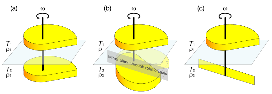
We turn to the question of how to configure the motor. Leaving the exact choice of the shape for later, we tackle the following the question: if we have a certain part of the motor in one reservoir, how will the placement of the part in the other reservoir effect the motion of the motor We start by proposing three simple constructions (see Fig. 5):

  1. 1.

    The shapes are identical in both reservoirs (Fig. 5a). This includes the location of the rotation axis with respect to the shape. The exact shape can be determined afterwards. With

    𝑑l1r2contour-integraldifferential-dsubscript𝑙1superscriptsubscript𝑟parallel-to2\displaystyle\oint dl_{1}r_{\shortparallel}^{2} =𝑑l2r2absentcontour-integraldifferential-dsubscript𝑙2superscriptsubscript𝑟parallel-to2\displaystyle=\oint dl_{2}r_{\shortparallel}^{2} =𝑑lr2,absentcontour-integraldifferential-d𝑙superscriptsubscript𝑟parallel-to2\displaystyle=\oint dlr_{\shortparallel}^{2}, (45)
    𝑑l1r3contour-integraldifferential-dsubscript𝑙1superscriptsubscript𝑟parallel-to3\displaystyle\oint dl_{1}r_{\shortparallel}^{3} =𝑑l2r3absentcontour-integraldifferential-dsubscript𝑙2superscriptsubscript𝑟parallel-to3\displaystyle=\oint dl_{2}r_{\shortparallel}^{3} =𝑑lr3,absentcontour-integraldifferential-d𝑙superscriptsubscript𝑟parallel-to3\displaystyle=\oint dlr_{\shortparallel}^{3}, (46)

    Eq. [44] simplifies to

    ω=2πkBm4Iρ1ρ2(T21/2T11/2)(T2T1)(ρ1T11/2+ρ2T21/2)2𝑑lr3𝑑lr2.delimited-⟨⟩𝜔2𝜋subscript𝑘𝐵𝑚4𝐼subscript𝜌1subscript𝜌2superscriptsubscript𝑇212superscriptsubscript𝑇112subscript𝑇2subscript𝑇1superscriptsubscript𝜌1superscriptsubscript𝑇112subscript𝜌2superscriptsubscript𝑇2122contour-integraldifferential-d𝑙superscriptsubscript𝑟parallel-to3contour-integraldifferential-d𝑙superscriptsubscript𝑟parallel-to2\langle\omega\rangle=\frac{\sqrt{2\pi k_{B}m}}{4I}\frac{\rho_{1}\rho_{2}(T_{2}^{1/2}-T_{1}^{1/2})(T_{2}-T_{1})}{(\rho_{1}T_{1}^{1/2}+\rho_{2}T_{2}^{1/2})^{2}}\frac{\oint dl\,r_{\shortparallel}^{3}}{\oint dl\,r_{\shortparallel}^{2}}. (47)
    Refer to caption
    Figure 5: Three possible configurations of the motor parts in a two-reservoir system. In (a) the part in the first reservoir is copied exactly to the other reservoir. Not only the shapes are identical, also their position relative to the rotation axis. In (b) the motor part in one reservoir is reflected in the other reservoir. The reflecting plane passes through the rotation axis. In (c) a general shape is combined with a blade: a plane of length L𝐿L (and height H𝐻H in three dimensions). Note that the system is rotationally invariant in each reservoir separately.
  2. 2.

    The shapes are still general but they are exact mirror images of each other in both reservoirs (Fig. 5b). Also the location of the rotation axis with respect to the shape is mirrored. The mirror axis (plane) is through the rotation axis, but its orientation is of no importance, as our system is rotationally invariant. Writing

    𝑑l1r2contour-integraldifferential-dsubscript𝑙1superscriptsubscript𝑟parallel-to2\displaystyle\oint dl_{1}r_{\shortparallel}^{2} =𝑑l2r2absentcontour-integraldifferential-dsubscript𝑙2superscriptsubscript𝑟parallel-to2\displaystyle=\oint dl_{2}r_{\shortparallel}^{2} =𝑑lr2,absentcontour-integraldifferential-d𝑙superscriptsubscript𝑟parallel-to2\displaystyle=\oint dlr_{\shortparallel}^{2}, (48)
    𝑑l1r3contour-integraldifferential-dsubscript𝑙1superscriptsubscript𝑟parallel-to3\displaystyle\oint dl_{1}r_{\shortparallel}^{3} =𝑑l2r3absentcontour-integraldifferential-dsubscript𝑙2superscriptsubscript𝑟parallel-to3\displaystyle=-\oint dl_{2}r_{\shortparallel}^{3} =𝑑lr3,absentcontour-integraldifferential-d𝑙superscriptsubscript𝑟parallel-to3\displaystyle=\oint dlr_{\shortparallel}^{3}, (49)

    Eq. [44] now becomes

    ω=2πkBm4Iρ1ρ2(T21/2+T11/2)(T2T1)(ρ1T11/2+ρ2T21/2)2𝑑lr3𝑑lr2.delimited-⟨⟩𝜔2𝜋subscript𝑘𝐵𝑚4𝐼subscript𝜌1subscript𝜌2superscriptsubscript𝑇212superscriptsubscript𝑇112subscript𝑇2subscript𝑇1superscriptsubscript𝜌1superscriptsubscript𝑇112subscript𝜌2superscriptsubscript𝑇2122contour-integraldifferential-d𝑙superscriptsubscript𝑟parallel-to3contour-integraldifferential-d𝑙superscriptsubscript𝑟parallel-to2\langle\omega\rangle=\frac{\sqrt{2\pi k_{B}m}}{4I}\frac{\rho_{1}\rho_{2}(T_{2}^{1/2}+T_{1}^{1/2})(T_{2}-T_{1})}{(\rho_{1}T_{1}^{1/2}+\rho_{2}T_{2}^{1/2})^{2}}\frac{\oint dl\,r_{\shortparallel}^{3}}{\oint dl\,r_{\shortparallel}^{2}}. (50)
  3. 3.

    We use a general (yet unknown) shape in the first reservoir, while in the second reservoir we put a blade of length L𝐿L, rotating about one end (Fig. 5c). Omitting the index i=1𝑖1i=1, and identifying

    𝑑l2r2contour-integraldifferential-dsubscript𝑙2superscriptsubscript𝑟parallel-to2\displaystyle\oint dl_{2}r_{\shortparallel}^{2} =2L3/3,absent2superscript𝐿33\displaystyle=2L^{3}/3, (51)
    𝑑l2r3contour-integraldifferential-dsubscript𝑙2superscriptsubscript𝑟parallel-to3\displaystyle\oint dl_{2}r_{\shortparallel}^{3} =0,absent0\displaystyle=0, (52)

    we obtain

    ω=2πkBm4Iρ1ρ2T21/2(T2T1)(2L3/3)𝑑lr3(ρ1T11/2𝑑lr2+ρ2T21/2(2L3/3))2.delimited-⟨⟩𝜔2𝜋subscript𝑘𝐵𝑚4𝐼subscript𝜌1subscript𝜌2superscriptsubscript𝑇212subscript𝑇2subscript𝑇12superscript𝐿33contour-integraldifferential-d𝑙superscriptsubscript𝑟parallel-to3superscriptsubscript𝜌1superscriptsubscript𝑇112contour-integraldifferential-d𝑙superscriptsubscript𝑟parallel-to2subscript𝜌2superscriptsubscript𝑇2122superscript𝐿332\langle\omega\rangle=\frac{\sqrt{2\pi k_{B}m}}{4I}\frac{\rho_{1}\rho_{2}T_{2}^{1/2}(T_{2}-T_{1})(2L^{3}/3)\oint dl\,r_{\shortparallel}^{3}}{(\rho_{1}T_{1}^{1/2}\oint dl\,r_{\shortparallel}^{2}+\rho_{2}T_{2}^{1/2}(2L^{3}/3))^{2}}. (53)

Comparing the three suggested configurations, we see configuration (1) is even when the temperature difference ΔT=T1T2Δ𝑇subscript𝑇1subscript𝑇2\Delta T=T_{1}-T_{2} is inverted, while (2) and (3) are odd. For small temperature differences, ωdelimited-⟨⟩𝜔\langle\omega\rangle is approximately parabolic in ΔTΔ𝑇\Delta T, while (2) and (3) are linear. For small ΔTΔ𝑇\Delta T therefore (1) yields much lower angular speeds than (2) and (3).

For a small temperature difference a rather technical calculation shows that the average angular velocity for configuration (2) is at least twice that of construction (3) for the same general shape with similar linear dimensions as the blade.

In a numerical procedure described later, we discovered that the configuration of two mirror shapes in the two reservoirs produces the maximal average angular velocity. In other words, given a certain part in one reservoir, the highest average angular velocity is obtained by using the reflected shape in the other reservoir.
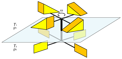
Refer to caption
Figure 6: A motor with multiple identical shapes in each reservoir. For the depicted configuration with equal multiples, n=m=4𝑛𝑚4n=m=4, we show that the resulting average angular velocity is the same as that for only one shape in each reservoir.

One could think of multiple but identical structures (blades) in each reservoir, as illustrated in Fig. 6. Ignoring the increased probability of multiple collisions of gas particles with the motor, our theory leads to an average angular velocity

ω=2πkBm4Iρ1ρ2(T2T1)(T21/2𝑑l1r3𝑑l2r2T11/2𝑑l2r3𝑑l1r2)(nmρ1T11/2𝑑l1r2+mnρ2T21/2𝑑l2r2)2,delimited-⟨⟩𝜔2𝜋subscript𝑘𝐵𝑚4𝐼subscript𝜌1subscript𝜌2subscript𝑇2subscript𝑇1superscriptsubscript𝑇212contour-integraldifferential-dsubscript𝑙1superscriptsubscript𝑟parallel-to3contour-integraldifferential-dsubscript𝑙2superscriptsubscript𝑟parallel-to2superscriptsubscript𝑇112contour-integraldifferential-dsubscript𝑙2superscriptsubscript𝑟parallel-to3contour-integraldifferential-dsubscript𝑙1superscriptsubscript𝑟parallel-to2superscript𝑛𝑚subscript𝜌1superscriptsubscript𝑇112contour-integraldifferential-dsubscript𝑙1superscriptsubscript𝑟parallel-to2𝑚𝑛subscript𝜌2superscriptsubscript𝑇212contour-integraldifferential-dsubscript𝑙2superscriptsubscript𝑟parallel-to22\langle\omega\rangle=\frac{\sqrt{2\pi k_{B}m}}{4I}\frac{\rho_{1}\rho_{2}(T_{2}-T_{1})\left(T_{2}^{1/2}\oint dl_{1}\,r_{\shortparallel}^{3}\oint dl_{2}\,r_{\shortparallel}^{2}-T_{1}^{1/2}\oint dl_{2}\,r_{\shortparallel}^{3}\oint dl_{1}\,r_{\shortparallel}^{2}\right)}{\left(\sqrt{\frac{n}{m}}\rho_{1}T_{1}^{1/2}\oint dl_{1}\,r_{\shortparallel}^{2}+\sqrt{\frac{m}{n}}\rho_{2}T_{2}^{1/2}\oint dl_{2}\,r_{\shortparallel}^{2}\right)^{2}}, (54)

for a system with n𝑛n identical blades in reservoir 1 and m𝑚m identical blades in reservoir 2. The appearing contour integrals are over one shape of the set of identical shapes. For the same number of shapes in both reservoirs, n=m𝑛𝑚n=m, the average angular velocity is the same as with only one blade in each reservoir. The result also shows that it is beneficial to have the highest number of blades in the reservoir with the highest ρT1/2𝑑lr2𝜌superscript𝑇12contour-integraldifferential-d𝑙superscriptsubscript𝑟parallel-to2\rho T^{1/2}\oint dl\,r_{\shortparallel}^{2} factor, or simply the highest ρT1/2𝜌superscript𝑇12\rho T^{1/2} factor if the blades have the same shape in both reservoirs.

VI.5 Globular proteins

Looking for real-world candidates to fill the role of our Brownian motor, we turn our attention to biological systems. In the further analysis we want to use physical values for the dimensions, masses and so on. A possibility is to apply our model to globular proteins, which could give the shape of the motor parts. The two parts would reside in a water environment, separated by a lipid membrane.

To obtain orders of magnitude for our results we will refer often to the values in Table 1.

Mass of one part M/2𝑀2M/2 1.66×10²²kg1.66superscript1022kg1.66\times 10^{-22}\text{kg}
Density of the motor ρmsubscript𝜌𝑚\rho_{m} 1380kg m31380superscriptkg m31380\>\text{kg m}^{-3}
Volume of one part V𝑉V 120 nm3superscriptnm3\text{nm}^{3}
Radius of one part (if assumed spherical) R𝑅R 3 nm
Particle mass (H2OsubscriptH2O\text{H}_{2}\text{O}) m𝑚m 2.992×1026kg2.992superscript1026kg2.992\times 10^{-26}\text{kg}
Reservoir temperature T1,T2subscript𝑇1subscript𝑇2T_{1},T_{2} ±300plus-or-minus300\pm 300 K
Reservoir particle density ρ1,ρ2subscript𝜌1subscript𝜌2\rho_{1},\rho_{2} ±3.3×1028m3plus-or-minus3.3superscript1028superscriptm3\pm 3.3\times 10^{28}\text{m}^{-3}
Table 1: Typical parameters used for the motor and environment. The values of the individual parts correspond to those of globular proteins.

VI.6 External parameters

Refer to caption
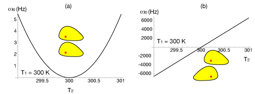
Figure 7: The temperature dependency of ω0subscript𝜔0\omega_{0} for a configuration of (a) identical shapes and of (b) mirror shapes in the two reservoirs. One reservoir is kept on a fixed temperature T1=300Ksubscript𝑇1300KT_{1}=300\text{K}, while the temperature T2subscript𝑇2T_{2} in the other reservoir changes in a range of 300±1Kplus-or-minus3001K300\pm 1\text{K}. For (a) we see a nearly parabolic dependency on T2T1subscript𝑇2subscript𝑇1T_{2}-T_{1}. The sense of rotation remains the same if we switch part 1 and part 2 of the motor, and the angular velocity is rather small. For (b) we see a much larger effect, a nearly linear dependency on T2T1subscript𝑇2subscript𝑇1T_{2}-T_{1}, and the sense of rotation is inverted by switching part 1 and part 2 of the motor. The densities are taken the same in both reservoirs.

In the cases of identical shapes and mirror shapes (Eqs. [47, 50]) we can separate from the expressions for ωdelimited-⟨⟩𝜔\langle\omega\rangle a shape-dependent factor,

𝒮=AMI𝑑lr3𝑑lr2.𝒮𝐴𝑀𝐼contour-integraldifferential-d𝑙superscriptsubscript𝑟parallel-to3contour-integraldifferential-d𝑙superscriptsubscript𝑟parallel-to2\mathcal{S}=\sqrt{A}\frac{M}{I}\frac{\oint dl\,r_{\shortparallel}^{3}}{\oint dl\,r_{\shortparallel}^{2}}. (55)

A factor A𝐴\sqrt{A} (or V1/3superscript𝑉13V^{1/3} if we prefer to work in three dimensions), which stands for the typical dimensions of a motor part, is multiplied to make 𝒮𝒮\mathcal{S} scale-invariant. 𝒮𝒮\mathcal{S} will be discussed in detail in the next section. Eqs. [47, 50] can then be written as

ω=ω0𝒮.delimited-⟨⟩𝜔subscript𝜔0𝒮\langle\omega\rangle=\omega_{0}\mathcal{S}. (56)

What remains is a factor ω0subscript𝜔0\omega_{0} that depends on the specific configuration, the reservoirs temperatures and densities, and the masses of the motor and particles:

ω0=ω0±=2πkBm4MAρ1ρ2(T21/2T11/2)(T2T1)(ρ1T11/2+ρ2T21/2)2.subscript𝜔0superscriptsubscript𝜔0plus-or-minus2𝜋subscript𝑘𝐵𝑚4𝑀𝐴subscript𝜌1subscript𝜌2minus-or-plussuperscriptsubscript𝑇212superscriptsubscript𝑇112subscript𝑇2subscript𝑇1superscriptsubscript𝜌1superscriptsubscript𝑇112subscript𝜌2superscriptsubscript𝑇2122\omega_{0}=\omega_{0}^{\pm}=\frac{\sqrt{2\pi k_{B}m}}{4M\sqrt{A}}\frac{\rho_{1}\rho_{2}(T_{2}^{1/2}\mp T_{1}^{1/2})(T_{2}-T_{1})}{(\rho_{1}T_{1}^{1/2}+\rho_{2}T_{2}^{1/2})^{2}}. (57)

We have used the notation ω0+superscriptsubscript𝜔0\omega_{0}^{+} for the configuration with two identical shapes in the two reservoirs and ω0superscriptsubscript𝜔0\omega_{0}^{-} for the configuration where the shapes are mirror images.

ω0subscript𝜔0\omega_{0} is also dependent of the size of the motor. Because the mass M𝑀M of the motor is also size-dependent, the full dependency could be written as MA=2ρmA3/2𝑀𝐴2subscript𝜌𝑚superscript𝐴32M\sqrt{A}=2\rho_{m}A^{3/2} in two dimensions, or MV1/3=2ρmV4/3𝑀superscript𝑉132subscript𝜌𝑚superscript𝑉43MV^{1/3}=2\rho_{m}V^{4/3} in three dimensions, if the density ρmsubscript𝜌𝑚\rho_{m} of the motor interior is considered constant. Therefore ω0M3/2proportional-tosubscript𝜔0superscript𝑀32\omega_{0}\propto M^{-3/2} in two dimensions and ω0M4/3proportional-tosubscript𝜔0superscript𝑀43\omega_{0}\propto M^{-4/3} in three dimensions.

Fig. 7 shows the temperature dependency of ω0subscript𝜔0\omega_{0}, calculated with the physical values of Table 1 and equal reservoir densities. As mentioned before ω0superscriptsubscript𝜔0\omega_{0}^{-} is linear in T2T1subscript𝑇2subscript𝑇1T_{2}-T_{1}, while ω0+superscriptsubscript𝜔0\omega_{0}^{+} is quadratic.

VI.7 Shape factor

Next, we consider the size-independent geometrical factor,

𝒮=AMI𝑑lr3𝑑lr2,𝒮𝐴𝑀𝐼contour-integraldifferential-d𝑙superscriptsubscript𝑟parallel-to3contour-integraldifferential-d𝑙superscriptsubscript𝑟parallel-to2\mathcal{S}=\sqrt{A}\frac{M}{I}\frac{\oint dl\,r_{\shortparallel}^{3}}{\oint dl\,r_{\shortparallel}^{2}}, (58)

which is comprised of an interior factor M/I𝑀𝐼M/I, and an exterior (boundary) factor 𝑑lr3/𝑑lr2contour-integraldifferential-d𝑙superscriptsubscript𝑟parallel-to3contour-integraldifferential-d𝑙superscriptsubscript𝑟parallel-to2\oint dl\,r_{\shortparallel}^{3}/\oint dl\,r_{\shortparallel}^{2}

The factor M/I𝑀𝐼M/I is actually independent of the mass of the motor because the inertial moment I𝐼I is proportional to the mass M𝑀M. It only describes the spacial distribution of mass. For a homogeneous motor interior it is given by

MI=iAiir2𝑑Ai.𝑀𝐼subscript𝑖subscript𝐴𝑖subscript𝑖superscript𝑟2differential-dsubscript𝐴𝑖\frac{M}{I}=\frac{\sum_{i}A_{i}}{\sum_{i}\int r^{2}dA_{i}}. (59)

The integral is over the entire interior of the motor, and r𝑟r is the distance of an interior point to the rotation axis.

Finally the factor 𝑑lr3/𝑑lr2contour-integraldifferential-d𝑙superscriptsubscript𝑟parallel-to3contour-integraldifferential-d𝑙superscriptsubscript𝑟parallel-to2\oint dl\,r_{\shortparallel}^{3}/\oint dl\,r_{\shortparallel}^{2} depends on the exact form of the boundary of the motor parts, where rsubscript𝑟parallel-tor_{\shortparallel} is to be measured from the location of the rotation axis. The integrals are over the entire boundary.

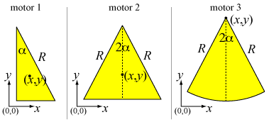
To enable us to get an understanding of the geometrical factor, we introduce three simple realizations (Fig. 8) (in two dimensions and with homogeneous mass distributions), of which the boundary can easily be described analytically. For these prototype shapes all factors can be expressed in closed form.
Refer to caption
Figure 8: Three simple shapes for the motor parts. All all determined by a minimal number of parameters. The shape is determined by the angle α𝛼\alpha, the size by one side R𝑅R, and the position with respect to the rotation axis (at the origin) by one coordinate (x,y)𝑥𝑦(x,y). For the triangles (Motor 1: right triangle; Motor 2: isosceles triangle) (x,y)𝑥𝑦(x,y) is the location of the center of mass, while for the disk sector (Motor 3) (x,y)𝑥𝑦(x,y) corresponds to the center of the disk.

The shape of the motors parts are respectively a right triangle (Motor 1), an isosceles triangle (Motor 2) and a disk sector (Motor 3). Both the dimensions of the motor parts (R𝑅R) and the shape (α𝛼\alpha) are fixed with one parameter, making a comparative study easier. We would also like to specify the location of the motor part relative to the rotation axis with one representative point with coordinate (x,y)𝑥𝑦(x,y). For motors 1 and 2 we choose the center of mass and for motor 3 the center of the disk sector (see (Fig. 8)) as this representative point . For these simple motors we can calculate analytical expressions for 𝑑lr2contour-integraldifferential-d𝑙superscriptsubscript𝑟parallel-to2\oint dl\,r_{\shortparallel}^{2} and 𝑑lr3contour-integraldifferential-d𝑙superscriptsubscript𝑟parallel-to3\oint dl\,r_{\shortparallel}^{3}. As these expressions are rather long, and the details are not of immediate relevance, we have put them in the appendix. As an example consider the Motor 2 case:

dlr2=2R9(R2+3Rycos3α+9y2+9x2sinα+sin2α(R2(3sinα2cos2α)+9x29y2)),contour-integral𝑑𝑙superscriptsubscript𝑟parallel-to22𝑅9superscript𝑅23𝑅𝑦3𝛼9superscript𝑦29superscript𝑥2𝛼superscript2𝛼superscript𝑅23𝛼22𝛼9superscript𝑥29superscript𝑦2\oint dl\,r_{\shortparallel}^{2}=\frac{2R}{9}\biggl{(}R^{2}+3Ry\cos 3\alpha+9y^{2}+9x^{2}\sin\alpha\\ +\sin^{2}\alpha\left(R^{2}(3\sin\alpha-2\cos 2\alpha)+9x^{2}-9y^{2}\right)\biggr{)}, (60)

and

dlr3=R3xsin2α(R(3y+Rcosα)(12cos2α)+3(x23y2)cosα).contour-integral𝑑𝑙superscriptsubscript𝑟parallel-to3𝑅3𝑥2𝛼𝑅3𝑦𝑅𝛼122𝛼3superscript𝑥23superscript𝑦2𝛼\oint dl\,r_{\shortparallel}^{3}=\frac{R}{3}x\sin 2\alpha\biggl{(}R(3y+R\cos\alpha)(1-2\cos 2\alpha)\\ +3\left(x^{2}-3y^{2}\right)\cos\alpha\biggr{)}. (61)

The intertial moments I𝐼I for the three motors are given in Table 2.

Motor 1 I/M=R2/18+x2+y2𝐼𝑀superscript𝑅218superscript𝑥2superscript𝑦2I/M=R^{2}/18+x^{2}+y^{2}
Motor 2 I/M=R2(2cos2α)/18+x2+y2𝐼𝑀superscript𝑅222𝛼18superscript𝑥2superscript𝑦2I/M=R^{2}(2-\cos 2\alpha)/18+x^{2}+y^{2}
Motor 3 I/M=R224Rysinα3α+x2+y2𝐼𝑀superscript𝑅224𝑅𝑦𝛼3𝛼superscript𝑥2superscript𝑦2I/M=\frac{R^{2}}{2}-\frac{4Ry\sin\alpha}{3\alpha}+x^{2}+y^{2}
Table 2: The ratio of the inertial moment I𝐼I over the mass M𝑀M of the motors in Fig. 8 given as a function of the location (x,y)𝑥𝑦(x,y) (of the center of mass for Motors 1 and 2, and of the center of the disk for Motor 3) with respect to the rotation axis and the shape parameters, angle α𝛼\alpha and size R𝑅R. The distribution of mass within the motors is assumed homogeneous.

Some physical properties are immediately apparent from these expressions. For example 𝑑lr3contour-integraldifferential-d𝑙superscriptsubscript𝑟parallel-to3\oint dl\,r_{\shortparallel}^{3}, and hence the angular velocity ωdelimited-⟨⟩𝜔\langle\omega\rangle, is zero when

  • x=0𝑥0x=0: this is when the rotation axis is on the symmetry axis of the motor; there is no preferred sense of rotation,

  • sin2α=02𝛼0\sin 2\alpha=0 or α=0𝛼0\alpha=0 or α=π/2𝛼𝜋2\alpha=\pi/2: the motor is bar shaped, and loses its asymmetry (or chirality).

Note that 𝑑lr2contour-integraldifferential-d𝑙superscriptsubscript𝑟parallel-to2\oint dl\,r_{\shortparallel}^{2}, which also appears as a factor in the expression for the friction coefficient, is not zero if the shape is bar shaped (or symmtrical in general).

In general the 𝑑lr3contour-integraldifferential-d𝑙superscriptsubscript𝑟parallel-to3\oint dl\,r_{\shortparallel}^{3} factor (Eq. 61 for Motor 2) describes the asymmetry of the motor. It also determines the sense of rotation. For example for Motor 2, the rotation sense is inverted when the rotation axis is placed on opposite sides of the symmetry axis, x=x0𝑥subscript𝑥0x=x_{0} and x=x0𝑥subscript𝑥0x=-x_{0}.

Refer to caption
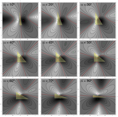
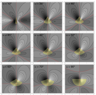
Figure 9: Contour plots of the average angular velocity ω(x,y)delimited-⟨⟩𝜔𝑥𝑦\langle\omega\rangle(x,y) of Motor 1 as a function of the location of the rotation axis (x,y)𝑥𝑦(x,y), for several values of the angle α𝛼\alpha. The center of mass of the motor is in the origin (0,0)00(0,0). Regions in black (and white) correspond to locations for the rotation axis that yield the highest ωdelimited-⟨⟩𝜔\langle\omega\rangle (but in opposite sense). If the rotation axis is put on a red curve there is zero average rotation. Maxima in ω(x,y)delimited-⟨⟩𝜔𝑥𝑦\langle\omega\rangle(x,y) are marked by dots, the purple dot reveals the optimal place for the rotation axis (the one that gives the highest angular velocity). Note that one red curve for the α=45𝛼superscript45\alpha=45^{\circ} realisation corresponds with a symmetry axis of the shape. The motor will not show directed motion if the axis is place there. Note also that mirror shapes (such as α=20𝛼superscript20\alpha=20^{\circ} and α=70𝛼superscript70\alpha=70^{\circ}) show opposite rotation sense, for all locations (x,y)𝑥𝑦(x,y).
Refer to caption
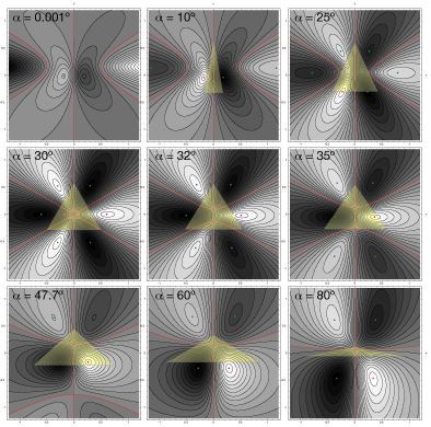
Figure 10: Contour plots of the average angular velocity ω(x,y)delimited-⟨⟩𝜔𝑥𝑦\langle\omega\rangle(x,y) of Motor 2 as a function of the location of the rotation axis (x,y)𝑥𝑦(x,y), for several values of the angle α𝛼\alpha. For a technical explanation see Fig. 9. The symmetry of the shape is reflected in the ω(x,y)delimited-⟨⟩𝜔𝑥𝑦\langle\omega\rangle(x,y) plot, in particular in the locations for the rotation axis that correspond to zero average angular velocity (red curves): the y𝑦y-axis for all the configurations and three symmetry axes for α=30𝛼superscript30\alpha=30^{\circ}. Note that the rotation sense is opposite for locations on opposite sides of a symmetry axis.
Refer to caption
Figure 11: Contour plots of the average angular velocity ω(x,y)delimited-⟨⟩𝜔𝑥𝑦\langle\omega\rangle(x,y) of Motor 3 as a function of the location of the rotation axis (x,y)𝑥𝑦(x,y), for several values of the angle α𝛼\alpha. For a technical explanation see Fig. 9.

More features can be seen from plots of the angular velocity of the motors as a function of their shape and configuration, see Figs. 9 (Motor 1), 10 (Motor 2) and 11 (Motor 3). Note that a coordinate change was made, xx,yyformulae-sequence𝑥𝑥𝑦𝑦x\rightarrow-x,y\rightarrow-y. This means the coordinate (x,y)𝑥𝑦(x,y) in the plot corresponds to the location of the rotation axis with respect to the representative point of the motor (center of mass or center of the disk), which is put in the origin of the plots. Figs. 9, 10, 11 of ω(x,y)delimited-⟨⟩𝜔𝑥𝑦\langle\omega\rangle(x,y) show lines of equal angular velocity (in black) and lines of zero average angular velocity (in red). Highest angular velocities are found in the black and white regions (but with opposite rotation sense). Local extrema of ω(x,y)delimited-⟨⟩𝜔𝑥𝑦\langle\omega\rangle(x,y) are represented by a green dot while a purple dot is the optimal location of the rotation axis. The shape of the motor is drawn in yellow.

We see that the red curves that signify zero average rotation can be straight lines when they correspond to a symmetry axis of the shape (the y𝑦y-axis in Figs. 10, 11 for all shapes α𝛼\alpha, but also in Fig. 9 for α=45𝛼superscript45\alpha=45^{\circ} for example), but in general they follow a curved path. The regions of opposite rotation sense, separated from each other by the red curves, form not so trivial patterns.

Also interesting to note is that the location of the rotation axis that yields the highest rotation speed is always in the vicinity of the rotating Brownian motor and often in its interior. Remember that the geometrical results are scale-invariant, and the relative locations of the maxima (and zero lines) are independent of the dimensions of the motor.

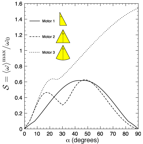
For certain choices of the shape and especially of the location of the rotation axis the average rotation speed can become zero. It is therefore sensible to investigate which configurations yield the highest rotation speed. For the three simple motor realizations, we determine the location of the rotation axis that yields the highest shape factor 𝒮𝒮\mathcal{S} for every value of the shape parameter α𝛼\alpha, as shown in Fig. 12.

Refer to caption
Figure 12: For the simple motor types (Fig. 8), we determined the position of the rotation axis that maximizes the average rotation speed for every shape, given by angle α𝛼\alpha. The values of α𝛼\alpha for which the shape factor 𝒮𝒮\mathcal{S} reaches a maximum are given in Table 3. It becomes clear that the shape is a key factor in the operation of the motor.

The angle α𝛼\alpha that results in the highest 𝒮𝒮\mathcal{S} is listed in Table 3 for each of the motors. The corresponding shapes are depicted in Fig. 13.

Refer to caption
Figure 13: The choices for the shape and location of the rotation axis for each of the three motor realizations that result in the highest average angular velocity of the motor. The location of the rotation axis is marked by a star. Although the initial constraints for Motor 1 and 2 are different (respectively the shape of a right and isosceles triangle), in their optimal configuration they are very similar. Motor 3 is optimal in the shape of a semi-disk, while we excluded the possibility of a concave shape.
Motor Angle α𝛼\alpha shape factor 𝒮𝒮\mathcal{S}
Motor 1 43.2 - 0.618
46.8 0.618
Motor 2 17.7 0.465
47.7 0.627
Motor 3 22.4 0.638
90.0 1.54
Table 3: For each of the three simple motor protypes, we shape factor 𝒮𝒮\mathcal{S} that corresponds to the optimal settings (shape and location of the rotation axis) is listed. The related shapes are shown in Fig. 13.

Considering the constraints put on the shape, Motor 1 and Motor 2 adopt very similar configurations, while the best (convex) shape for Motor 3 is a semi-disk.

VI.8 Optimal shape

The three motor realizations show that the angular velocity is sensitive to the precise shape of the motor. We are interested to know what happens if we relax the shape constraints while optimizing for maximum rotation speed. We solve this problem using a numerical procedure.

The boundary of the motor is modeled as piecewise linear. It is defined by the location of n𝑛n vertices. The numerical procedure finds the optimum location of the n𝑛n vertices, yielding maximum angular velocity, under the constraints that (1) the mass M𝑀M remains constant, (2) the shape remains convex. The mass constraint for a homogeneous mass distribution translates into conservation of total area A𝐴A. For low numbers n=3,4,5,6𝑛3456n=3,4,5,6 the optimum location of the vertices is shown in Fig. 14.
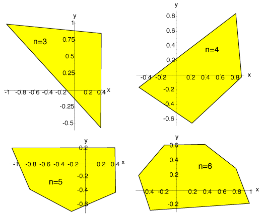
Refer to caption
Figure 14: A numerical procedure was used to find optimum piecewise linear shapes, by determining the best location of each vertex. The results for a small number of vertices, n=3,4,5,6𝑛3456n=3,4,5,6 are shown. Note that the results are invariant for rotations with respect the rotation axis, which is located in the origin (0,0)00(0,0) of the coordinate system.

Note that the rotation axis is still fixed in the origin (0,0)00(0,0).

By increasing the number of vertices n𝑛n, the piecewise linear shape approaches the smooth boundary that yields the highest angular velocity possible.
Refer to caption
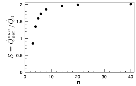
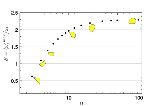
Figure 15: The shape factor 𝒮𝒮\mathcal{S} is a scale-invariant measure of the influence of the precise geometry of the motor. For 𝒮=0𝒮0\mathcal{S}=0, the average angular velocity is zero. A numerical procedure was used to obtain the optimum shape (with highest 𝒮𝒮\mathcal{S}) for a motor shape that is piecewise linear, i. e. consisting of n𝑛n vertices connected by straight lines. For high n𝑛n we find an approximation of the exact optimum shape and a lower limit of the maximal 𝒮𝒮\mathcal{S} that can be obtained. 𝒮𝒮\mathcal{S} converges to a value of about 2.29. A negative 𝒮𝒮\mathcal{S} is possible, but this corresponds to a shape that is the mirror image of the shape with opposite 𝒮𝒮\mathcal{S}.

In Fig. 15 the shape factor 𝒮𝒮\mathcal{S} is plot against the number of vertices n𝑛n. We see a convergence for large n𝑛n. For n=100𝑛100n=100 the value of 𝒮𝒮\mathcal{S} is 2.29. This is a factor 3.65 higher than the best value for a triangular shape, n=3𝑛3n=3, 𝒮=0.63𝒮0.63\mathcal{S}=0.63. The corresponding shape (for n=100𝑛100n=100) is shown in Fig. 16.

Refer to caption
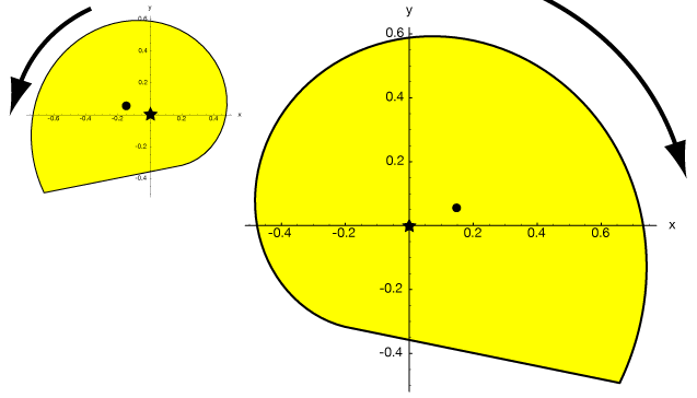
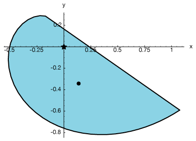
Figure 16: The (two-dimensional) shape of one motor part that produces the highest average angular velocity, found with a numerical procedure. The rotation axis is marked by a star (at (0,0)00(0,0)), while the center of mass is marked by a dot. The shape in the larger figure rotates from the y𝑦y-axis to the x𝑥x-axis, while its mirror shape (enantiomer) in the smaller figure rotates in the opposite sense. The area of the shape is normalized to 1.

A tentative explanation for the optimum spiral shape is that it combines a long curved section with small rsubscript𝑟parallel-tor_{\shortparallel} (and hence small friction) with a short section that is linear, providing the necessary propulsion.

The chirality of the shape determines the rotation sense. A motor that consists of two identical optimum shapes as shown in the large figure of Fig. 16 actually has a negative 𝒮𝒮\mathcal{S}. This means the motor rotates clockwise (from y𝑦y-axis to x𝑥x-axis). Its enantiomer (the small figure) has positive 𝒮𝒮\mathcal{S} and rotates counterclockwise (from x𝑥x-axis to y𝑦y-axis).

We initially applied the numerical procedure to identical shapes in the two reservoirs. We knew we would simultaneously find the optimum shape for the construction with mirrored shapes in both reservoirs as they share the same shape factor 𝒮𝒮\mathcal{S} (see Eqs. 47 and 50). Then we extended the numerical procedure so that the shapes in each reservoir could develop independently. For a small temperature difference (ΔT=1Δ𝑇1\Delta T=1 K) the shapes become almost exactly each others mirror image (area difference A1/A2=1.00045subscript𝐴1subscript𝐴21.00045A_{1}/A_{2}=1.00045). Even for a large temperature difference (ΔT=100Δ𝑇100\Delta T=100 K) we find mirror shapes with only a small area discrepancy (A1/A2=1.017subscript𝐴1subscript𝐴21.017A_{1}/A_{2}=1.017). The larger shape is in the reservoir with lower temperature. To obtain a positive rotation sense (from x𝑥x-axis to y𝑦y-axis) of the motor for a construction with mirror images, the shape with positive 𝒮𝒮\mathcal{S} needs to be placed in the cold reservoir , while its mirror shape with negative 𝒮𝒮\mathcal{S} (but equal in absolute value) should be in the warm reservoir.

VI.9 Physical estimates for the Brownian rotor

We have now collected all the necessary elements to estimate the physical properties of our motor. In a real world example of course many of the features discussed in this paper will only be of qualitative use.

We learned that is is advantageous to use a configuration where the shape of the motor in one reservoir is the mirror image of the shape in the other reservoir (section VI.4). We also found the optimal individual shape (section VI.8). In the results we present here we assume these optimizations can be approached.

When we use the physical properties of small protein structures in an environment of water molecules (section VI.5) as the separate building blocks of our motors we arrive at an average angular velocity of about 1500 Hz when driven by a temperature gradient of 0.1 K (T1=300subscript𝑇1300T_{1}=300 K, T2=300.1subscript𝑇2300.1T_{2}=300.1 K). This corresponds to about 230 rotations per second.

VII Cross processes

We discussed a Brownian motor, and derived a relationship between its motion – the average angular velocity ωdelimited-⟨⟩𝜔\langle\omega\rangle – and the applied temperature difference ΔTΔ𝑇\Delta T. This relationship is an example of a cross process. The normal process that would give rise to a motion ωdelimited-⟨⟩𝜔\langle\omega\rangle originates from a mechanical force. In our system with only a rotational degree of freedom this mechanical force would be in the form of a torque τ𝜏\tau along the z𝑧z-axis.

Cross processes are very common in physics. One well-known example is the Seebeck effect callen , where a temperature difference over an electric conductor causes an electric current. The Seebeck effect has a reverse or mirror cross process: the Peltier effect. Here, an applied electric current causes a temperature difference. Processes and their mirror processes are related through a general principle of stability. In the example of the Seebeck-Peltier effects, consider a system that is originally in equilibrium. If it is perturbed by the application of a temperature gradient, currents will start to flow (the Seebeck effect), which in turn will give rise to a counteracting temperature difference (the Peltier effect), attempting to cancel out the original cause of the disturbance. Another example is Lenz’ law in electromagnetism. Moving a ferromagnetic core into a coil will induce currents in the coil. These currents are such that the resulting magnetic field will expel the core, hence counteracting the original disturbance.

Now that we established the existence of a cross process in the Brownian motor system and showed the relationship between a cross process and its mirror process, the question naturally arises: what is the mirror process in our system? It should be one that counteracts the original perturbation – a temperature difference between the reservoirs. A flow of heat Q˙12subscript˙𝑄12\dot{Q}_{1\rightarrow 2} from reservoir 1 to reservoir 2 would do exactly that. And we know the normal process (that causes rotational motion) is induced by a torque τ𝜏\tau. The mirror cross process then is a heat flow caused by a torque. When we perturb our system in temperature equilibrium by applying a torque τ𝜏\tau, the motor will of course rotate. How can the system react to counterbalance this motion? By creating a temperature gradient between the two reservoirs, that according to the theory of the Brownian motor will cause rotational motion. The sign of the temperature difference is such that the resulting rectified Brownian motion opposes the motion started by the torque.

VIII Model of the Brownian Refrigerator
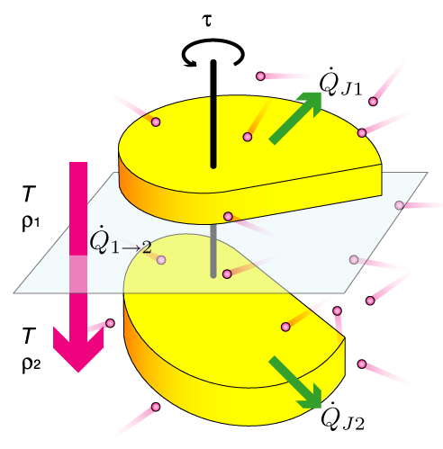
Refer to caption
Figure 17: The Brownian refrigerator is a rotating device consisting of two connected bodies, each in a temperature reservoir. By applying a torque on the apparatus, a heat flow Q˙12subscript˙𝑄12\dot{Q}_{1\rightarrow 2} will arise that can cool down reservoir 1 at the expense of heating up reservoir 2. It is possible to obtain the conditions where this cooling power is larger than the dissipative heating Q˙J1subscript˙𝑄𝐽1\dot{Q}_{J1}.

We propose a cooling apparatus or refrigerator based on the Brownian motor described before. Two reservoirs (see Fig. 17) are thermally isolated from each other and initially at temperature equilibrium, T1=T2=Tsubscript𝑇1subscript𝑇2𝑇T_{1}=T_{2}=T. The refrigerator consists of a rotating device with a part in each reservoir. The parts are rigidly connected via a rotation axis and are subject to random collisions with particles in their reservoirs. These have mass m𝑚m, considered much smaller than the total mass M𝑀M of the rotating device. On applying a torque τ𝜏\tau along the z𝑧z-axis the system will develop a heat flow Q˙12subscript˙𝑄12\dot{Q}_{1\rightarrow 2}, cooling reservoir 1 down at the expense of heating up reservoir 2. The following derivation of this heat flow is done for a construction where one part of the device is the reflected copy of the other (as in Fig. 5b) because it shows a linear response in small temperature differences T1T2subscript𝑇1subscript𝑇2T_{1}-T_{2} and it produces the highest rotating speeds and resulting heat flow.

IX Linear response and Onsager symmetry

Previously we derived a relation between the average angular velocity ωdelimited-⟨⟩𝜔\langle\omega\rangle of the rotating brownian motor and the temperatures of the two isolated reservoirs, T1subscript𝑇1T_{1} and T2subscript𝑇2T_{2}, correct to order m/M𝑚𝑀m/M:

ω=2πkBm4Iρ1ρ2(T21/2+T11/2)(T2T1)(ρ1T11/2+ρ2T21/2)2𝑑lr3𝑑lr2.delimited-⟨⟩𝜔2𝜋subscript𝑘𝐵𝑚4𝐼subscript𝜌1subscript𝜌2superscriptsubscript𝑇212superscriptsubscript𝑇112subscript𝑇2subscript𝑇1superscriptsubscript𝜌1superscriptsubscript𝑇112subscript𝜌2superscriptsubscript𝑇2122contour-integraldifferential-d𝑙superscriptsubscript𝑟parallel-to3contour-integraldifferential-d𝑙superscriptsubscript𝑟parallel-to2\langle\omega\rangle=\frac{\sqrt{2\pi k_{B}m}}{4I}\frac{\rho_{1}\rho_{2}(T_{2}^{1/2}+T_{1}^{1/2})(T_{2}-T_{1})}{(\rho_{1}T_{1}^{1/2}+\rho_{2}T_{2}^{1/2})^{2}}\frac{\oint dl\,r_{\shortparallel}^{3}}{\oint dl\,r_{\shortparallel}^{2}}. (62)

Here I𝐼I is the inertial moment of the motor with respect to its rotation axis and 𝑑lr3/𝑑lr2contour-integraldifferential-d𝑙superscriptsubscript𝑟parallel-to3contour-integraldifferential-d𝑙superscriptsubscript𝑟parallel-to2\oint dl\,r_{\shortparallel}^{3}/\oint dl\,r_{\shortparallel}^{2} is a geometrical factor defined by the shape of the rotating motor parts. The geometrical factor is zero in a symmetrical configuration, hence the importance of choosing appropriate asymmetric or chiral elements. For a more detailed discussion of the geometrical factor we refer to Section VI.7. For a small temperature difference ΔTΔ𝑇\Delta T between the two reservoirs,

T1subscript𝑇1\displaystyle T_{1} =TΔT/2,absent𝑇Δ𝑇2\displaystyle=T-\Delta T/2, ΔTΔ𝑇\displaystyle\quad\Delta T =T2T1T,absentsubscript𝑇2subscript𝑇1much-less-than𝑇\displaystyle=T_{2}-T_{1}\ll T, (63)
T2subscript𝑇2\displaystyle T_{2} =T+ΔT/2,absent𝑇Δ𝑇2\displaystyle=T+\Delta T/2, T𝑇\displaystyle\quad T =(T1+T2)/2,absentsubscript𝑇1subscript𝑇22\displaystyle=(T_{1}+T_{2})/2, (64)

the mechanical response ωdelimited-⟨⟩𝜔\langle\omega\rangle is linear in ΔTΔ𝑇\Delta T to very good approximation:

ω2πkBm2Iρ1ρ2(ρ1+ρ2)2𝑑lr3𝑑lr2ΔTT1/2.delimited-⟨⟩𝜔2𝜋subscript𝑘𝐵𝑚2𝐼subscript𝜌1subscript𝜌2superscriptsubscript𝜌1subscript𝜌22contour-integraldifferential-d𝑙superscriptsubscript𝑟parallel-to3contour-integraldifferential-d𝑙superscriptsubscript𝑟parallel-to2Δ𝑇superscript𝑇12\langle\omega\rangle\approx\frac{\sqrt{2\pi k_{B}m}}{2I}\frac{\rho_{1}\rho_{2}}{(\rho_{1}+\rho_{2})^{2}}\frac{\oint dl\,r_{\shortparallel}^{3}}{\oint dl\,r_{\shortparallel}^{2}}\frac{\Delta T}{T^{1/2}}. (65)

An elegant way to calculate the cooling potential of our system is by making use of Onsager’s relations onsager . We will identify a flow and a force for the two cross processes involved.The alternative is to revisit the analysis of Section III, adding an extra torque term to the master equation. For the mechanical process we identify a flow J1=ωsubscript𝐽1delimited-⟨⟩𝜔J_{1}=\langle\omega\rangle and a thermodynamic force X2=ΔT/T2subscript𝑋2Δ𝑇superscript𝑇2X_{2}=\Delta T/T^{2} in the linear relation of Eq. 65. The proportionality constant L12subscript𝐿12L_{12} of the first Onsager relation,

J1=L12X2,subscript𝐽1subscript𝐿12subscript𝑋2J_{1}=L_{12}X_{2}, (66)

is, for our particular system, given by

L12=2πkBm2Iρ1ρ2(ρ1+ρ2)2T3/2𝑑lr3𝑑lr2.subscript𝐿122𝜋subscript𝑘𝐵𝑚2𝐼subscript𝜌1subscript𝜌2superscriptsubscript𝜌1subscript𝜌22superscript𝑇32contour-integraldifferential-d𝑙superscriptsubscript𝑟parallel-to3contour-integraldifferential-d𝑙superscriptsubscript𝑟parallel-to2L_{12}=\frac{\sqrt{2\pi k_{B}m}}{2I}\frac{\rho_{1}\rho_{2}}{(\rho_{1}+\rho_{2})^{2}}T^{3/2}\frac{\oint dl\,r_{\shortparallel}^{3}}{\oint dl\,r_{\shortparallel}^{2}}. (67)

For the second cross process, the cooling process, we can identify a heat flow J2=Q˙12subscript𝐽2subscript˙𝑄12J_{2}=\dot{Q}_{1\rightarrow 2}. The force X1subscript𝑋1X_{1} is given by the chemical potential associated with the particle flow J1=ωsubscript𝐽1delimited-⟨⟩𝜔J_{1}=\langle\omega\rangle of the normal process, and is generated by the application of the torque τ𝜏\tau. More precisely, X1=τ/Tsubscript𝑋1𝜏𝑇X_{1}=\tau/T. Again we expect a linear response

J2=L21X1.subscript𝐽2subscript𝐿21subscript𝑋1J_{2}=L_{21}X_{1}. (68)

Onsager symmetry now tells us that the two proportionality coefficients of the cross processes are identical,

L21=L12.subscript𝐿21subscript𝐿12L_{21}=L_{12}. (69)

The heat flow from one reservoir to the other in the linear regime now becomes obvious,

Q˙12=2πkBmT2Iρ1ρ2(ρ1+ρ2)2𝑑lr3𝑑lr2τ.subscript˙𝑄122𝜋subscript𝑘𝐵𝑚𝑇2𝐼subscript𝜌1subscript𝜌2superscriptsubscript𝜌1subscript𝜌22contour-integraldifferential-d𝑙superscriptsubscript𝑟parallel-to3contour-integraldifferential-d𝑙superscriptsubscript𝑟parallel-to2𝜏\dot{Q}_{1\rightarrow 2}=\frac{\sqrt{2\pi k_{B}mT}}{2I}\frac{\rho_{1}\rho_{2}}{(\rho_{1}+\rho_{2})^{2}}\frac{\oint dl\,r_{\shortparallel}^{3}}{\oint dl\,r_{\shortparallel}^{2}}\,\tau. (70)

The complete Onsager relations, combining normal and cross processes, are given by:

J1=L11X1+L12X2,J2=L21X1+L22X2.formulae-sequencesubscript𝐽1subscript𝐿11subscript𝑋1subscript𝐿12subscript𝑋2subscript𝐽2subscript𝐿21subscript𝑋1subscript𝐿22subscript𝑋2J_{1}=L_{11}X_{1}+L_{12}X_{2},\quad J_{2}=L_{21}X_{1}+L_{22}X_{2}. (71)

The Onsager coefficients we have not identified yet are:

L11=T/γ,L22=γ1γ2kBT2γI,formulae-sequencesubscript𝐿11𝑇𝛾subscript𝐿22subscript𝛾1subscript𝛾2subscript𝑘𝐵superscript𝑇2𝛾𝐼L_{11}=T/\gamma,\quad L_{22}=\frac{\gamma_{1}\gamma_{2}k_{B}T^{2}}{\gamma I}, (72)

while J1=ωsubscript𝐽1delimited-⟨⟩𝜔J_{1}=\langle\omega\rangle, J2=Q˙12subscript𝐽2subscript˙𝑄12J_{2}=\dot{Q}_{1\rightarrow 2}, X1=τ/Tsubscript𝑋1𝜏𝑇X_{1}=\tau/T, and X2=ΔT/T2subscript𝑋2Δ𝑇superscript𝑇2X_{2}=\Delta T/T^{2} as before. L11subscript𝐿11L_{11} can be associated to the direct mechanical response of the motor to the application of a torque, while L22subscript𝐿22L_{22} is related to heat conductivity, being the coefficient between the heat flow and the temperature gradient.

X Results and discussion
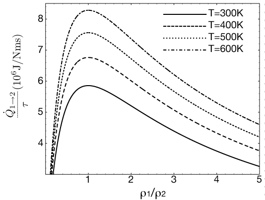
Refer to caption
Figure 18: Physical values of the cooling power Q˙12subscript˙𝑄12\dot{Q}_{1\rightarrow 2} of the Brownian refrigerator in response to a torque τ𝜏\tau are given for an environment of two nitrogen gas reservoirs for several choices of the temperature T𝑇T of the gases. The device works best when the densities of the gases, ρ1subscript𝜌1\rho_{1} and ρ2subscript𝜌2\rho_{2}, are equal. The mass of the gas particles is m=5×1026kg𝑚5superscript1026kgm=5\times 10^{-26}\text{kg}, while the mass of the device is M=1.66×10²²kg𝑀1.66superscript1022kgM=1.66\times 10^{-22}\text{kg}.

Eq. 70 gives us a relation between the heat flow from reservoir 1 to reservoir 2 and the applied torque. Earlier we chose the parameters of the building blocks that constitute our motor and its environment to be comparable with globular proteins in water, see Table 1 for details. Using these variables again for the refrigerating device we obtain a heat flow Q˙12subscript˙𝑄12\dot{Q}_{1\rightarrow 2} of 4.5 μ𝜇\muJ/s for every pNm of torque applied. This result is for T=300𝑇300T=300 K and a shape that is close to optimal. Note that in the ratio Q˙12/τsubscript˙𝑄12𝜏\dot{Q}_{1\rightarrow 2}/\tau, the geometrical factor,

MI𝑑lr3𝑑lr2,𝑀𝐼contour-integraldifferential-d𝑙superscriptsubscript𝑟parallel-to3contour-integraldifferential-d𝑙superscriptsubscript𝑟parallel-to2\frac{M}{I}\frac{\oint dl\,r_{\shortparallel}^{3}}{\oint dl\,r_{\shortparallel}^{2}}, (73)

found earlier reappears so that the comprehensive discussion therein (sections VI.7 and VI.8) remains applicable for the various shapes the parts of the refrigerator can adopt.

Fig. 18 shows the dependency of the cooling power Q˙12/τsubscript˙𝑄12𝜏\dot{Q}_{1\rightarrow 2}/\tau on the densities ρ1subscript𝜌1\rho_{1} and ρ2subscript𝜌2\rho_{2} of the gas reservoirs for different gas temperatures T𝑇T. Here we have set the cooling device in the membrane separating two gaseous environments (the values for nitrogen gas N2subscriptN2\text{N}_{2} are used: m=5×1026kg𝑚5superscript1026kgm=5\times 10^{-26}\text{kg}, while for the refrigerator M=1.66×10²²kg𝑀1.66superscript1022kgM=1.66\times 10^{-22}\text{kg} and typical radius 3 nm). The size of the effect is determined by the ratio of the gas densities ρ1/ρ2subscript𝜌1subscript𝜌2\rho_{1}/\rho_{2}. For all temperatures maximal cooling power is found when the densities in the two reservoirs are equal, ρ1=ρ2subscript𝜌1subscript𝜌2\rho_{1}=\rho_{2}. Higher heat fluxes arise when the gas temperature T𝑇T is higher.

The maximal torque that can be applied and the maximum obtainable temperature difference will be determined by increasing dissipative heat flows, which we discuss now.

X.1 Joule dissipation

We showed the occurrence of a heat flux Q˙12subscript˙𝑄12\dot{Q}_{1\rightarrow 2} that takes away heat from reservoir 1 to reservoir 2. Friction however will cause Joule heating in both reservoirs i=1,2𝑖12i=1,2 by an amount

Q˙Ji=γiω2=γiτ2/γ2.subscript˙𝑄𝐽𝑖subscript𝛾𝑖superscriptdelimited-⟨⟩𝜔2subscript𝛾𝑖superscript𝜏2superscript𝛾2\dot{Q}_{Ji}=\gamma_{i}\langle\omega\rangle^{2}=\gamma_{i}\tau^{2}/\gamma^{2}. (74)

If we want reservoir 1 to cool down, the heat Q˙12subscript˙𝑄12\dot{Q}_{1\rightarrow 2} transferred from reservoir 1 to 2 needs to be larger than the heat Q˙J1subscript˙𝑄𝐽1\dot{Q}_{J1} dissipated by friction in reservoir 1,

Q˙12Q˙J1=2kBTmIρ2τ𝑑lr3>1.subscript˙𝑄12subscript˙𝑄𝐽12subscript𝑘𝐵𝑇𝑚𝐼subscript𝜌2𝜏contour-integraldifferential-d𝑙superscriptsubscript𝑟parallel-to31\frac{\dot{Q}_{1\rightarrow 2}}{\dot{Q}_{J1}}=2\frac{k_{B}Tm}{I}\frac{\rho_{2}}{\tau}\oint dl\,r_{\shortparallel}^{3}>1. (75)

This condition poses a limit on the applied torque:

τ<τlim=2kBTmIρ2𝑑lr3.𝜏subscript𝜏lim2subscript𝑘𝐵𝑇𝑚𝐼subscript𝜌2contour-integraldifferential-d𝑙superscriptsubscript𝑟parallel-to3\tau<\tau_{\text{lim}}=2\frac{k_{B}Tm}{I}\rho_{2}\oint dl\,r_{\shortparallel}^{3}. (76)

A greater torque would cause the heat dissipation to annihilate the cooling effect. We are able to suggest a scale-invariant numerical limit for the torque. Note that both the inertial moment I𝐼I and the shape factor 𝑑lr3contour-integraldifferential-d𝑙superscriptsubscript𝑟parallel-to3\oint dl\,r_{\shortparallel}^{3} scale with R4superscript𝑅4R^{4} (R𝑅R being the typical linear dimension of the refrigerator) in the case that the refrigerator parts have homogeneous density ρmsubscript𝜌𝑚\rho_{m}. If we assume optimum operation using the appropriate chiral shapes of the parts, as will be developed in detail later (section X.2), we find

ρm𝑑lr3I=1.30684.subscript𝜌𝑚contour-integraldifferential-d𝑙superscriptsubscript𝑟parallel-to3𝐼1.30684\rho_{m}\frac{\oint dl\,r_{\shortparallel}^{3}}{I}=1.30684. (77)

This result depends only on the geometry and not on the dimensions of the parts. It will be lower for less favorable shapes and zero for a symmetric construction. The maximal torque than can be expressed as

τlim=2kBTρ2mρm×1.30684.subscript𝜏lim2subscript𝑘𝐵𝑇subscript𝜌2𝑚subscript𝜌𝑚1.30684\tau_{\text{lim}}=2k_{B}T\frac{\rho_{2}m}{\rho_{m}}\times 1.30684. (78)

This maximal torque is proportional to the ratio of the mass density ρ2msubscript𝜌2𝑚\rho_{2}m of gas that is heated and of the refrigerator ρmsubscript𝜌𝑚\rho_{m}. It does not depend on the size of cooling device. For T=300𝑇300T=300 K and a system according to Table 1, assuming optimum shape,

τlim=3.92×10²¹Nm.subscript𝜏lim3.92superscript1021Nm\tau_{\text{lim}}=3.92\times 10^{-21}\text{Nm}. (79)

X.2 Maximal net cooling

The cooling power of the refrigerator is proportional to the applied torque τ𝜏\tau (Eq. 70), while the dissipative heat flux grows with τ2superscript𝜏2\tau^{2} (Eq. 74). For large τ𝜏\tau the cooling effect will be annihilated by dissipation and in the previous section we calculated a cut-off τlimsubscript𝜏lim\tau_{\text{lim}}, at which both effects cancel each other. We can also calculate the torque τmaxsubscript𝜏max\tau_{\text{max}} that maximizes the net cooling,

Q˙net=Q˙12Q˙J1.subscript˙𝑄netsubscript˙𝑄12subscript˙𝑄𝐽1\dot{Q}_{\text{net}}=\dot{Q}_{1\rightarrow 2}-\dot{Q}_{J1}. (80)

A simple calculation leads to a maximum of Q˙net=AτBτ2subscript˙𝑄net𝐴𝜏𝐵superscript𝜏2\dot{Q}_{\text{net}}=A\tau-B\tau^{2} at τmax=τlim/2=A/(2B)subscript𝜏maxsubscript𝜏lim2𝐴2𝐵\tau_{\text{max}}=\tau_{\text{lim}}/2=A/(2B), with A=(2πkBmT)/(2I)(ρ1ρ2)/((ρ1+ρ2)2)(𝑑lr3)/(𝑑lr2)𝐴2𝜋subscript𝑘𝐵𝑚𝑇2𝐼subscript𝜌1subscript𝜌2superscriptsubscript𝜌1subscript𝜌22contour-integraldifferential-d𝑙superscriptsubscript𝑟parallel-to3contour-integraldifferential-d𝑙superscriptsubscript𝑟parallel-to2A=(\sqrt{2\pi k_{B}mT})/(2I)(\rho_{1}\rho_{2})/((\rho_{1}+\rho_{2})^{2})(\oint dl\,r_{\shortparallel}^{3})/(\oint dl\,r_{\shortparallel}^{2}) and B=γ1/γ𝐵subscript𝛾1𝛾B=\gamma_{1}/\gamma. For the optimum torque then we find:

τmax=kBTmIρ2𝑑lr3.subscript𝜏maxsubscript𝑘𝐵𝑇𝑚𝐼subscript𝜌2contour-integraldifferential-d𝑙superscriptsubscript𝑟parallel-to3\tau_{\text{max}}=\frac{k_{B}Tm}{I}\rho_{2}\oint dl\,r_{\shortparallel}^{3}. (81)

This result, like τlimsubscript𝜏lim\tau_{\text{lim}}, is independent of the size of the refrigerator (assuming a homogeneous interior). It only depends on the density of the the environment and the refrigerator, the environment temperature and the specific shape of the refrigerator. For an optimum shape (see later) and variables according to Table 1 we find:

τmax=1.96×10²¹Nm.subscript𝜏max1.96superscript1021Nm\tau_{\text{max}}=1.96\times 10^{-21}\text{Nm}. (82)

Substituting the explicit expression for τmaxsubscript𝜏max\tau_{\text{max}} into Eq. 80 yields the maximal net heat flow out of reservoir 1:

Q˙netmax=π8(kBTm)3/2I2ρ1ρ22(ρ1+ρ2)2(𝑑lr3)2𝑑lr2.superscriptsubscript˙𝑄netmax𝜋8superscriptsubscript𝑘𝐵𝑇𝑚32superscript𝐼2subscript𝜌1superscriptsubscript𝜌22superscriptsubscript𝜌1subscript𝜌22superscriptcontour-integraldifferential-d𝑙superscriptsubscript𝑟parallel-to32contour-integraldifferential-d𝑙superscriptsubscript𝑟parallel-to2\dot{Q}_{\text{net}}^{\text{max}}=\frac{\sqrt{\pi}}{8}\frac{(k_{B}Tm)^{3/2}}{I^{2}}\frac{\rho_{1}\rho_{2}^{2}}{(\rho_{1}+\rho_{2})^{2}}\frac{\left(\oint dl\,r_{\shortparallel}^{3}\right)^{2}}{\oint dl\,r_{\shortparallel}^{2}}. (83)

We see that when we also take into account the loss through friction, the refrigerator is most effective when the densities are the same in both reservoirs, ρ1=ρ2subscript𝜌1subscript𝜌2\rho_{1}=\rho_{2}. The net cooling is higher when the device works in higher gas densities. The reason may seem counterintuitive: the heat dissipation through friction is smaller in an environment with higher friction. Eq. 74 shows that the dissipated heat is proportional to the square of the average angular velocity ωdelimited-⟨⟩𝜔\langle\omega\rangle that is obtained by applying a torque τ𝜏\tau, and this velocity is lower when the friction γ𝛾\gamma is higher.

Before we can give numerical results, we need to investigate the role of the geometry of the refrigerator. We separate a scale-invariant shape factor from Eq. 83,

𝒮=1AM2I2(𝑑lr3)2𝑑lr2,𝒮1𝐴superscript𝑀2superscript𝐼2superscriptcontour-integraldifferential-d𝑙superscriptsubscript𝑟parallel-to32contour-integraldifferential-d𝑙superscriptsubscript𝑟parallel-to2\mathcal{S}=\frac{1}{\sqrt{A}}\frac{M^{2}}{I^{2}}\frac{\left(\oint dl\,r_{\shortparallel}^{3}\right)^{2}}{\oint dl\,r_{\shortparallel}^{2}}, (84)

where A𝐴A is the area of one part of the construction. All the factors that depend on the shape, the contours and the inertial moment, are included in 𝒮𝒮\mathcal{S}. We will begin straight away with optimizing this shape factor, and for most of the realizations of the refrigerator presented in this paper we assume the shape is (close to) optimum. The calculations however can also be done for other (less favorable) shapes; the elements of the calculation are comparable to those presented earlier, where we also discussed three simple model shapes that can be analyzed analytically. A similar numerical procedure as was used to find the optimal shape of the motor (see section VI.8), yields a value for 𝒮𝒮\mathcal{S}, see Fig. 19.

Refer to caption
Figure 19: The effectiveness of the refrigerator is influenced by its (chiral) shape. 𝒮𝒮\mathcal{S} gives a size-independent measure of this geometrical factor. With a numerical procedure we can optimize this factor, by approximating the shape of the motor parts as piecewise linear, with n𝑛n edges. For n𝑛n sufficiently high we approach the highest obtainable factor 𝒮𝒮\mathcal{S}, and the corresponding shape is represented in Fig. 20.

The procedure approximates the shape of the refrigerator parts as piecewise linear with n𝑛n vertices. For sufficiently large n𝑛n, 𝒮𝒮\mathcal{S} converges to a value slightly higher than 2. The corresponding optimum shape for the cooling function is then also found, see Fig. 20. The shape is that of a part of the refrigerator in one reservoir; placing the mirrored shape in the other reservoir gives the optimum configuration of the refrigerator. The axis of rotation is given by the z𝑧z-axis.

Refer to caption
Figure 20: The shape of one part of the refrigerating device that maximizes the net cooling power, which also takes into account the frictional dissipation. The complete device consists of this shape in one reservoir and the mirror image of this shape in the other. The two parts are rigidly connected with each other by a rotation axis, marked by a star. The mass distribution in the interior of the parts is assumed homogeneous. The center of mass is represented by a dot.

The numerical procedure expects the mass M𝑀M of the motor to be homogeneously distributed, which reflects the reality of biological entities such as proteins that could function as parts of the device.

For a homogeneous mass distribution we write the mass of the refrigerator as M=2ρmA𝑀2subscript𝜌𝑚𝐴M=2\rho_{m}A, with ρmsubscript𝜌𝑚\rho_{m} the constant density of the refrigerator parts. To find the maximum net heat flux the numerical factor 𝒮𝒮\mathcal{S} is multiplied by

Q˙0=2π16(kBTm)3/2ρm2A3/2ρ1ρ22(ρ1+ρ2)2,subscript˙𝑄02𝜋16superscriptsubscript𝑘𝐵𝑇𝑚32superscriptsubscript𝜌𝑚2superscript𝐴32subscript𝜌1superscriptsubscript𝜌22superscriptsubscript𝜌1subscript𝜌22\dot{Q}_{0}=\frac{\sqrt{2\pi}}{16}\frac{(k_{B}Tm)^{3/2}}{\rho_{m}^{2}A^{3/2}}\frac{\rho_{1}\rho_{2}^{2}}{(\rho_{1}+\rho_{2})^{2}}, (85)

so that Q˙netmax=Q˙0𝒮superscriptsubscript˙𝑄netmaxsubscript˙𝑄0𝒮\dot{Q}_{\text{net}}^{\text{max}}=\dot{Q}_{0}\mathcal{S}. Remember that our theory is two-dimensional. The result however depends on the absolute values of the gas densities ρ1subscript𝜌1\rho_{1} and ρ2subscript𝜌2\rho_{2}, contrary to Eq. 70 where only their relative magnitudes play a part . We cannot simply insert values for three-dimensional gas densities. Therefore we make a small technical detour to describe the three-dimensional expressions and justify for which case the two-dimensional shape optimization remains valid.

X.3 Three-dimensional model

In a three-dimensional analysis the essential difference is the description of the geometrical factors. Instead of a contour integral 𝑑lcontour-integraldifferential-d𝑙\oint dl there is an integral 𝑑Sdifferential-d𝑆\int dS over the surface of the refrigerator parts, while the vector rsubscript𝑟parallel-tor_{\shortparallel} gets a new definition, see Section V for details. For the ratio of the cooling power over the applied torque we find

Q˙12τ=2πkBmT2Iρ1ρ2(ρ1+ρ2)2𝑑Sr3𝑑Sr2,subscript˙𝑄12𝜏2𝜋subscript𝑘𝐵𝑚𝑇2𝐼subscript𝜌1subscript𝜌2superscriptsubscript𝜌1subscript𝜌22differential-d𝑆superscriptsubscript𝑟parallel-to3differential-d𝑆superscriptsubscript𝑟parallel-to2\frac{\dot{Q}_{1\rightarrow 2}}{\tau}=\frac{\sqrt{2\pi k_{B}mT}}{2I}\frac{\rho_{1}\rho_{2}}{(\rho_{1}+\rho_{2})^{2}}\frac{\int dS\,r_{\shortparallel}^{3}}{\int dS\,r_{\shortparallel}^{2}}, (86)

while the maximum net cooling power of reservoir 1 now becomes

Q˙netmax=π8(kBTm)3/2I2ρ1ρ22(ρ1+ρ2)2(𝑑Sr3)2𝑑Sr2.superscriptsubscript˙𝑄netmax𝜋8superscriptsubscript𝑘𝐵𝑇𝑚32superscript𝐼2subscript𝜌1superscriptsubscript𝜌22superscriptsubscript𝜌1subscript𝜌22superscriptdifferential-d𝑆superscriptsubscript𝑟parallel-to32differential-d𝑆superscriptsubscript𝑟parallel-to2\dot{Q}_{\text{net}}^{\text{max}}=\frac{\sqrt{\pi}}{8}\frac{(k_{B}Tm)^{3/2}}{I^{2}}\frac{\rho_{1}\rho_{2}^{2}}{(\rho_{1}+\rho_{2})^{2}}\frac{\left(\int dS\,r_{\shortparallel}^{3}\right)^{2}}{\int dS\,r_{\shortparallel}^{2}}. (87)

We again use a product of an external Q˙0subscript˙𝑄0\dot{Q}_{0} and a scale-invariant geometrical factor 𝒮𝒮\mathcal{S},

Q˙netmax=Q˙0𝒮.superscriptsubscript˙𝑄netmaxsubscript˙𝑄0𝒮\dot{Q}_{\text{net}}^{\text{max}}=\dot{Q}_{0}\mathcal{S}. (88)

The geometrical factor now needs to be scaled by a factor proportional to R2superscript𝑅2R^{2}, with R𝑅R the typical linear dimension of the shape. For this we use V2/3superscript𝑉23V^{2/3}, with V𝑉V the volume of a refrigerator part:

𝒮=1V2/3M2I2(𝑑Sr3)2𝑑Sr2,𝒮1superscript𝑉23superscript𝑀2superscript𝐼2superscriptdifferential-d𝑆superscriptsubscript𝑟parallel-to32differential-d𝑆superscriptsubscript𝑟parallel-to2\mathcal{S}=\frac{1}{V^{2/3}}\frac{M^{2}}{I^{2}}\frac{\left(\int dS\,r_{\shortparallel}^{3}\right)^{2}}{\int dS\,r_{\shortparallel}^{2}}, (89)

The shape factor can then be solved analytically or numerically, producing size-independent results. The remaining factor

Q˙0subscript˙𝑄0\displaystyle\dot{Q}_{0} =π8(kBTm)3/2M2ρ1ρ22(ρ1+ρ2)2V2/3absent𝜋8superscriptsubscript𝑘𝐵𝑇𝑚32superscript𝑀2subscript𝜌1superscriptsubscript𝜌22superscriptsubscript𝜌1subscript𝜌22superscript𝑉23\displaystyle=\frac{\sqrt{\pi}}{8}\frac{(k_{B}Tm)^{3/2}}{M^{2}}\frac{\rho_{1}\rho_{2}^{2}}{(\rho_{1}+\rho_{2})^{2}}V^{2/3} (90)
=2π16(kBTm)3/2ρm2V4/3ρ1ρ22(ρ1+ρ2)2,absent2𝜋16superscriptsubscript𝑘𝐵𝑇𝑚32superscriptsubscript𝜌𝑚2superscript𝑉43subscript𝜌1superscriptsubscript𝜌22superscriptsubscript𝜌1subscript𝜌22\displaystyle=\frac{\sqrt{2\pi}}{16}\frac{(k_{B}Tm)^{3/2}}{\rho_{m}^{2}V^{4/3}}\frac{\rho_{1}\rho_{2}^{2}}{(\rho_{1}+\rho_{2})^{2}}, (91)

then shows again the role of the various parameters. In the second expression for Q˙0subscript˙𝑄0\dot{Q}_{0} we substituted M=2ρmV𝑀2subscript𝜌𝑚𝑉M=2\rho_{m}V for the homogeneous case.

We now argue that we can recuperate the two-dimensional optimization of the shape factor 𝒮𝒮\mathcal{S} and corresponding two-dimensional shape. We propose a prismatic structure for each of the refrigerator parts, defined by two equal, flat (two-dimensional) surfaces separated by a distance H𝐻H, as shown in the initial model of the device in Fig. 17. The rotation axis is perpendicular to the two surfaces. For this configuration it is easy to show that the surface integrals can be written as the product of the distance H𝐻H and the contour integral of the top or bottom surface, exactly as in the two-dimensional description:

𝑑Sr2differential-d𝑆superscriptsubscript𝑟parallel-to2\displaystyle\int dS\,r_{\shortparallel}^{2} =H𝑑lr,2D2,absent𝐻contour-integraldifferential-d𝑙superscriptsubscript𝑟parallel-to2𝐷2\displaystyle=H\oint dl\,r_{\shortparallel,2D}^{2}, (92)
𝑑Sr3differential-d𝑆superscriptsubscript𝑟parallel-to3\displaystyle\int dS\,r_{\shortparallel}^{3} =H𝑑lr,2D3.absent𝐻contour-integraldifferential-d𝑙superscriptsubscript𝑟parallel-to2𝐷3\displaystyle=H\oint dl\,r_{\shortparallel,2D}^{3}. (93)

Also, for a homogeneous mass distribution,

MI=Vr2𝑑V=HAHr2𝑑A,𝑀𝐼𝑉superscriptsubscript𝑟perpendicular-to2differential-d𝑉𝐻𝐴𝐻superscript𝑟2differential-d𝐴\frac{M}{I}=\frac{V}{\int r_{\perp}^{2}dV}=\frac{HA}{H\int r^{2}dA}, (94)

where we take the integral over the volume V𝑉V of rsubscript𝑟perpendicular-tor_{\perp}, the distance to the rotation axis, and find it is equivalent to taking the surface integral over the top or bottom surface A𝐴A of the prism times the thickness H𝐻H. In conclusion we recover the two-dimensional shapefactor (Eq. 84) by inserting the corresponding volume V=(HA)3/2𝑉superscript𝐻𝐴32V=(H\sqrt{A})^{3/2} in Eq. 89. The approach is then to use the three-dimensional expression for Q˙0subscript˙𝑄0\dot{Q}_{0} (Eq. 91), and the numerical results for the two-dimensional case, as in Fig. 19.
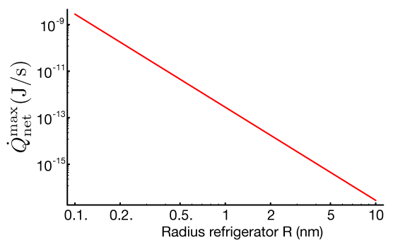
Refer to caption
Figure 21: The net cooling power of the Brownian refrigerator (the dissipative loss by friction is deducted from the heat flux that cools down one compartment) depends strongly on the size of the cooling device. Values for a device operating between two aquatic reservoirs (m=2.992×1026kg𝑚2.992superscript1026kgm=2.992\times 10^{-26}\text{kg}, ρ1=ρ2=3.343×1028m3subscript𝜌1subscript𝜌23.343superscript1028superscriptm3\rho_{1}=\rho_{2}=3.343\times 10^{28}\text{m}^{-3}) at temperature T=300K𝑇300KT=300\text{K} are presented here. The size-dependency of the mass of the rotating device M𝑀M is included, while its density is that of a typical protein, ρm=1380kg m3subscript𝜌𝑚1380superscriptkg m3\rho_{m}=1380\>\text{kg m}^{-3}.

Doing this for a temperature (T=300K𝑇300KT=300\text{K}), reservoir densities (ρ1=ρ2=3.343×1028m3subscript𝜌1subscript𝜌23.343superscript1028superscriptm3\rho_{1}=\rho_{2}=3.343\times 10^{28}\text{m}^{-3}) and m=2.992×1026kg𝑚2.992superscript1026kgm=2.992\times 10^{-26}\text{kg} for an aquatic environment, and ρm=1380kg m3subscript𝜌𝑚1380superscriptkg m3\rho_{m}=1380\>\text{kg m}^{-3}, typical for proteins, Q˙netmax=Q˙0𝒮superscriptsubscript˙𝑄netmaxsubscript˙𝑄0𝒮\dot{Q}_{\text{net}}^{\text{max}}=\dot{Q}_{0}\mathcal{S} can be expressed as a function of only the radius R𝑅R of one refrigerator part, as in Fig. 21. For a globular protein of typical dimension R3nm𝑅3nmR\approx 3\text{nm}, we find a value of Q˙netmax=3.5×10¹⁵J/ssuperscriptsubscript˙𝑄netmax3.5superscript1015Js\dot{Q}_{\text{net}}^{\text{max}}=3.5\times 10^{-15}\text{J}/\text{s}. Note the strong size dependence: a refrigerator of one nm, would yield a cooling power of about 2.8×10¹³J/s2.8superscript1013Js2.8\times 10^{-13}\text{J}/\text{s}. For comparison, it takes about 2.2×10¹²J2.2superscript1012J2.2\times 10^{-12}\text{J} to cool down a 1 μm𝜇m\mu\text{m} small cell one Kelvin, which could be accomplished by one refrigerator of 1 nm radius in one minute.

X.4 Thermal conductivity

As mentioned earlier, the L22subscript𝐿22L_{22} Onsager coefficient can be related to heat conductivity between the reservoirs. In the linear response model, the heat conducted from one reservoir to the other can be quantified:

Q˙cond=γ1γ2γIkBΔT.subscript˙𝑄condsubscript𝛾1subscript𝛾2𝛾𝐼subscript𝑘𝐵Δ𝑇\dot{Q}_{\text{cond}}=\frac{\gamma_{1}\gamma_{2}}{\gamma I}k_{B}\Delta T. (95)

Here γ1subscript𝛾1\gamma_{1} and γ2subscript𝛾2\gamma_{2} are the friction coefficients of the separate parts of the refrigerator, and γ=γ1+γ2𝛾subscript𝛾1subscript𝛾2\gamma=\gamma_{1}+\gamma_{2} represents the total friction coefficient.
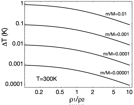
Refer to caption
Figure 22: The temperature gradient ΔTΔ𝑇\Delta T for which the conductive heat flow cancels the cooling heat flow. For the device to cool down reservoir 1 (at the expense of reservoir 2), the temperature difference must remain under this limit. The different curves are for examples of the mass ratios between colliding particle (m𝑚m) and device M𝑀M. A small M𝑀M (or large m𝑚m) is beneficial. The sustainable temperature gradient is highest for high gas density ρ2subscript𝜌2\rho_{2} in reservoir 2 (relative to ρ1subscript𝜌1\rho_{1}). For high gas density ρ1subscript𝜌1\rho_{1} in reservoir 1 the obtainable temperature gradient becomes very small. The graph is for absolute temperature differences around T=300𝑇300T=300 K.

The conductive heat flow is proportional to the temperature gradient ΔTΔ𝑇\Delta T and goes from the warm to the cold reservoir. Therefore it is directed against the cooling power of the device and for a temperature difference larger than ΔTlimΔsubscript𝑇lim\Delta T_{\text{lim}} the net cooling effect will vanish. The condition Q˙cond<Q˙netmaxsubscript˙𝑄condsuperscriptsubscript˙𝑄netmax\dot{Q}_{\text{cond}}<\dot{Q}_{\text{net}}^{\text{max}} leads to

ΔTT<π8mIρ2ρ1+ρ2(𝑑lr3)2(𝑑lr2)2.Δ𝑇𝑇𝜋8𝑚𝐼subscript𝜌2subscript𝜌1subscript𝜌2superscriptcontour-integraldifferential-d𝑙superscriptsubscript𝑟parallel-to32superscriptcontour-integraldifferential-d𝑙superscriptsubscript𝑟parallel-to22\frac{\Delta T}{T}<\frac{\pi}{8}\frac{m}{I}\frac{\rho_{2}}{\rho_{1}+\rho_{2}}\frac{\left(\oint dl\,r_{\shortparallel}^{3}\right)^{2}}{\left(\oint dl\,r_{\shortparallel}^{2}\right)^{2}}. (96)

Note that the sustainable temperature gradient is proportional to m/M𝑚𝑀m/M. In Fig. 22 we show ΔTlimΔsubscript𝑇lim\Delta T_{\text{lim}} for varying m/M𝑚𝑀m/M as a function of the density ratio ρ1/ρ2subscript𝜌1subscript𝜌2\rho_{1}/\rho_{2}. For our choice of the direction of the cooling effect (reservoir 1 cools down, reservoir 2 heats up), a higher relative density in reservoir 2 allows a larger ΔTlimΔsubscript𝑇lim\Delta T_{\text{lim}}. In the limit of ρ1subscript𝜌1\rho_{1} being much smaller than ρ2subscript𝜌2\rho_{2}, ΔTlim/TΔsubscript𝑇lim𝑇\Delta T_{\text{lim}}/T approaches (π/8)(m/I)(𝑑lr3)2/(𝑑lr2)2𝜋8𝑚𝐼superscriptcontour-integraldifferential-d𝑙superscriptsubscript𝑟parallel-to32superscriptcontour-integraldifferential-d𝑙superscriptsubscript𝑟parallel-to22(\pi/8)(m/I)\left(\oint dl\,r_{\shortparallel}^{3}\right)^{2}/\left(\oint dl\,r_{\shortparallel}^{2}\right)^{2} Earlier we found equal densities, ρ1=ρ2subscript𝜌1subscript𝜌2\rho_{1}=\rho_{2}, to correspond with maximum net cooling power, for which the maximum sustainable temperature gradient ΔTlimΔsubscript𝑇lim\Delta T_{\text{lim}} is half this value.

For the previously used example of globular proteins (see Table 1 for the parameters), ΔTlim=4.3Δsubscript𝑇lim4.3\Delta T_{\text{lim}}=4.3 mK at T=300𝑇300T=300 K and equal reservoir densities.

In all examples given, the shape is presumed to be (close to) optimal.

Appendix A Full expressions for model motors

For Motor 1 a straightforward calculation leads to

𝑑lr2contour-integraldifferential-d𝑙superscriptsubscript𝑟parallel-to2\displaystyle\oint dl\,r_{\shortparallel}^{2} =R72(R2cos4α\displaystyle=\frac{R}{72}\biggl{(}R^{2}\cos 4\alpha
+2R((R+6y)cos3α(R+6x)sin3α)2𝑅𝑅6𝑦3𝛼𝑅6𝑥3𝛼\displaystyle+2R\bigl{(}(R+6y)\cos 3\alpha-(R+6x)\sin 3\alpha\bigr{)}
+12((yx)(R+3(x+y))cos2α6xysin2α)12𝑦𝑥𝑅3𝑥𝑦2𝛼6𝑥𝑦2𝛼\displaystyle+12\bigl{(}(y-x)(R+3(x+y))\cos 2\alpha-6xy\sin 2\alpha\bigr{)}
+6((R2+2yR+12y2)cosα\displaystyle+6\bigl{(}(R^{2}+2yR+12y^{2})\cos\alpha
+(R2+2xR+12x2)sinα)\displaystyle+(R^{2}+2xR+12x^{2})\sin\alpha\bigr{)}
+7R2+12(x+y)R+36(x2+y2)),\displaystyle+7R^{2}+12(x+y)R+36(x^{2}+y^{2})\biggr{)}, (97)

while I/M=R2/18+x2+y2𝐼𝑀superscript𝑅218superscript𝑥2superscript𝑦2I/M=R^{2}/18+x^{2}+y^{2}. The friction coefficient is then directly obtained through Eq. (29). One can note that this coefficient is always nonzero, unless R=0𝑅0R=0. Also for α=0𝛼0\alpha=0, when the motor has the shape of two connected bars, Eq. (97) is nonzero. Choosing α=0𝛼0\alpha=0, x=0𝑥0x=0, and y=R/3𝑦𝑅3y=R/3, we retrieve the expression for a rod of length R𝑅R rotating about one end,

𝑑lr2=2R3/3.contour-integraldifferential-d𝑙superscriptsubscript𝑟parallel-to22superscript𝑅33\oint dl\,r_{\shortparallel}^{2}=2R^{3}/3. (98)

The sense of rotation is geometrically determined by

𝑑lr3contour-integraldifferential-d𝑙superscriptsubscript𝑟parallel-to3\displaystyle\oint dl\,r_{\shortparallel}^{3} =Rsin2α432(R3sin4α\displaystyle=-\frac{R\sin 2\alpha}{432}\biggl{(}R^{3}\sin 4\alpha
+18R2(xcos3α+ysin3α)18superscript𝑅2𝑥3𝛼𝑦3𝛼\displaystyle+18R^{2}\bigl{(}x\cos 3\alpha+y\sin 3\alpha\bigr{)}
+108R(2xycos2α(x2y2)sin2α)108𝑅2𝑥𝑦2𝛼superscript𝑥2superscript𝑦22𝛼\displaystyle+108R\bigl{(}2xy\cos 2\alpha-(x^{2}-y^{2})\sin 2\alpha\bigr{)}
+54(x(R24x2+12y2)cosα\displaystyle+54\bigl{(}x(R^{2}-4x^{2}+12y^{2})\cos\alpha
y(R2+12x24y2)sinα)).\displaystyle-y(R^{2}+12x^{2}-4y^{2})\sin\alpha\bigr{)}\biggr{)}. (99)

For a bar-shaped motor, α=0𝛼0\alpha=0 or α=90𝛼superscript90\alpha=90^{\circ}, Eq. (99) effectively returns zero, resulting is a zero average rotation for the motor. The shape needs to have chiral asymmetry for the motor to function. This observation becomes more apparent when we locate the rotation axis in the center of mass, (x,y)=(0,0)𝑥𝑦00(x,y)=(0,0). Then Eq. (99) simply becomes

𝑑lr3=R4432sin(2α)sin(4α),contour-integraldifferential-d𝑙superscriptsubscript𝑟parallel-to3superscript𝑅44322𝛼4𝛼\oint dl\,r_{\shortparallel}^{3}=-\frac{R^{4}}{432}\sin(2\alpha)\sin(4\alpha), (100)

which equals zero also when α=45𝛼superscript45\alpha=45^{\circ}. For this angle the shape contains an extra symmetry axis, lifting the chiral symmetry. To find a nonzero rotation, we need to change the shape to a chiral asymmetric one. We see an opposite rotation sense when moving across the symmetric position. In particular for this choice of the position of the rotation axis, we note that ω[π/2α]=ω[α]delimited-⟨⟩𝜔delimited-[]𝜋2𝛼delimited-⟨⟩𝜔delimited-[]𝛼\langle\omega\rangle[\pi/2-\alpha]=-\langle\omega\rangle[\alpha], where for this triangular shape, α𝛼\alpha and π/2α𝜋2𝛼\pi/2-\alpha correspond to chiral enantiomers. This is because 𝑑lr2contour-integraldifferential-d𝑙superscriptsubscript𝑟parallel-to2\oint dl\,r_{\shortparallel}^{2}, M/I𝑀𝐼M/I, and v0subscript𝑣0v_{0} are even under a απ/2α𝛼𝜋2𝛼\alpha\rightarrow\pi/2-\alpha transformation, while 𝑑lr3contour-integraldifferential-d𝑙superscriptsubscript𝑟parallel-to3\oint dl\,r_{\shortparallel}^{3} is uneven. For other locations of the rotation axis, we see a similar behavior. In Fig. 9 we show the dependency of the angular velocity ωdelimited-⟨⟩𝜔\langle\omega\rangle on the exact place of the axis (which in our calculations can be outside the motor body). For chiral shapes, the axis of rotation that yields zero rotation is no longer on a symmetry axis. These locations are generally given by three curves in the two-dimensional plane. Nonzero rotation is found in the six zones divided by the zero curves and the sense of rotation is opposite in neighboring zones. One point of maximal rotation speed is found per zone, actual and maximal values of ωdelimited-⟨⟩𝜔\langle\omega\rangle will be discussed later. To conclude our discussion of Motor 1, a few expressions for fixed values are given. For α=π/4𝛼𝜋4\alpha=\pi/4,

dlr2=R36((3+22)R2+6(x+y)R+18((1+2)x22yx+(1+2)y2)),contour-integral𝑑𝑙superscriptsubscript𝑟parallel-to2𝑅36322superscript𝑅26𝑥𝑦𝑅1812superscript𝑥22𝑦𝑥12superscript𝑦2\oint dl\,r_{\shortparallel}^{2}=\frac{R}{36}\biggl{(}\left(3+2\sqrt{2}\right)R^{2}+6(x+y)R\\ +18\left(\left(1+\sqrt{2}\right)x^{2}-2yx+\left(1+\sqrt{2}\right)y^{2}\right)\biggr{)}, (101)
𝑑lr3=R24(xy)×(6(x+y)R+62(x2+4yx+y2)2R2),contour-integraldifferential-d𝑙superscriptsubscript𝑟parallel-to3𝑅24𝑥𝑦6𝑥𝑦𝑅62superscript𝑥24𝑦𝑥superscript𝑦22superscript𝑅2\oint dl\,r_{\shortparallel}^{3}=\frac{R}{24}(x-y)\\ \times\left(6(x+y)R+6\sqrt{2}\left(x^{2}+4yx+y^{2}\right)-\sqrt{2}R^{2}\right), (102)

and for α=π/6𝛼𝜋6\alpha=\pi/6

dlr2=R48((5+23)R2+4(3+3)yR+36x2+12y((3+23)y23x)),contour-integral𝑑𝑙superscriptsubscript𝑟parallel-to2𝑅48523superscript𝑅2433𝑦𝑅36superscript𝑥212𝑦323𝑦23𝑥\oint dl\,r_{\shortparallel}^{2}=\frac{R}{48}\biggl{(}\left(5+2\sqrt{3}\right)R^{2}+4\left(3+\sqrt{3}\right)yR\\ +36x^{2}+12y\left(\left(3+2\sqrt{3}\right)y-2\sqrt{3}x\right)\biggr{)}, (103)
dlr3=R2883(3R32+18yR2+108xyR543(xy)(x+y)R27y(R2+12x24y2)+273x(R24x2+12y2)).contour-integral𝑑𝑙superscriptsubscript𝑟parallel-to3𝑅28833superscript𝑅3218𝑦superscript𝑅2108𝑥𝑦𝑅543𝑥𝑦𝑥𝑦𝑅27𝑦superscript𝑅212superscript𝑥24superscript𝑦2273𝑥superscript𝑅24superscript𝑥212superscript𝑦2\oint dl\,r_{\shortparallel}^{3}=-\frac{R}{288\sqrt{3}}\biggl{(}\frac{\sqrt{3}R^{3}}{2}+18yR^{2}+108xyR\\ -54\sqrt{3}(x-y)(x+y)R-27y\left(R^{2}+12x^{2}-4y^{2}\right)\\ +27\sqrt{3}x\left(R^{2}-4x^{2}+12y^{2}\right)\biggr{)}. (104)

Similarly for Motor 2 we find, again choosing the origin of the coordinate system (x,y)𝑥𝑦(x,y) in the center of mass of the motor,

dlr2=2R9(R2+3Rycos3α+9y2+9x2sinα+sin2α(R2(3sinα2cos2α)+9x29y2)),contour-integral𝑑𝑙superscriptsubscript𝑟parallel-to22𝑅9superscript𝑅23𝑅𝑦3𝛼9superscript𝑦29superscript𝑥2𝛼superscript2𝛼superscript𝑅23𝛼22𝛼9superscript𝑥29superscript𝑦2\oint dl\,r_{\shortparallel}^{2}=\frac{2R}{9}\biggl{(}R^{2}+3Ry\cos 3\alpha+9y^{2}+9x^{2}\sin\alpha\\ +\sin^{2}\alpha\left(R^{2}(3\sin\alpha-2\cos 2\alpha)+9x^{2}-9y^{2}\right)\biggr{)}, (105)

while I/M=R2(2cos2α)/18+x2+y2𝐼𝑀superscript𝑅222𝛼18superscript𝑥2superscript𝑦2I/M=R^{2}(2-\cos 2\alpha)/18+x^{2}+y^{2}. Again

dlr3=R3xsin2α(R(3y+Rcosα)(12cos2α)+3(x23y2)cosα)contour-integral𝑑𝑙superscriptsubscript𝑟parallel-to3𝑅3𝑥2𝛼𝑅3𝑦𝑅𝛼122𝛼3superscript𝑥23superscript𝑦2𝛼\oint dl\,r_{\shortparallel}^{3}=\frac{R}{3}x\sin 2\alpha\biggl{(}R(3y+R\cos\alpha)(1-2\cos 2\alpha)\\ +3\left(x^{2}-3y^{2}\right)\cos\alpha\biggr{)} (106)

determines the sense of rotation and reflects the chiral symmetry of the motor. Specifically, putting the rotation axis on the symmetry axis of the motor, x=0𝑥0x=0, results in a zero average rotation. Putting the axis on symmetrical location across the symmetry axis yields the same rotation speed, but in opposite sense, ω[x,y]=ω[x,y]delimited-⟨⟩𝜔𝑥𝑦delimited-⟨⟩𝜔𝑥𝑦\langle\omega\rangle[-x,y]=-\langle\omega\rangle[x,y]. Again, reducing the motor to a bar shaped object, α=0𝛼0\alpha=0 or α=π/2𝛼𝜋2\alpha=\pi/2, a preferred sense of rotation can no longer be determined and ω=0delimited-⟨⟩𝜔0\langle\omega\rangle=0. Fig. 10 shows ωdelimited-⟨⟩𝜔\langle\omega\rangle for general positions of the rotation axis, for different configurations of the motor shape. For certain configurations the expressions simplify to reflect a higher symmetry. For α=π/6𝛼𝜋6\alpha=\pi/6 for example the shape is that of an equilateral triangle with side 2R2𝑅2R, with

𝑑lr2=14R(R2+6(x2+y2)),contour-integraldifferential-d𝑙superscriptsubscript𝑟parallel-to214𝑅superscript𝑅26superscript𝑥2superscript𝑦2\oint dl\,r_{\shortparallel}^{2}=\frac{1}{4}R\left(R^{2}+6\left(x^{2}+y^{2}\right)\right), (107)

and

𝑑lr3=34Rx(x23y2),contour-integraldifferential-d𝑙superscriptsubscript𝑟parallel-to334𝑅𝑥superscript𝑥23superscript𝑦2\oint dl\,r_{\shortparallel}^{3}=\frac{3}{4}Rx\left(x^{2}-3y^{2}\right), (108)

so that the full expression for the rotation speed becomes

ω=v036x(x23y2)R4+18(x2+y2)R2+72(x2+y2)2.delimited-⟨⟩𝜔subscript𝑣036𝑥superscript𝑥23superscript𝑦2superscript𝑅418superscript𝑥2superscript𝑦2superscript𝑅272superscriptsuperscript𝑥2superscript𝑦22\langle\omega\rangle=v_{0}\frac{36x\left(x^{2}-3y^{2}\right)}{R^{4}+18\left(x^{2}+y^{2}\right)R^{2}+72\left(x^{2}+y^{2}\right)^{2}}. (109)

The rotation speed will be zero, when the rotation axis is on any of the three symmetry axes of the equilateral triangle, x=±3y𝑥plus-or-minus3𝑦x=\pm\sqrt{3}y besides x=0𝑥0x=0, while the extrema are located on the vertices of a regular hexagon of side (3+33)/6R3336𝑅\sqrt{(3+\sqrt{33})/6}R. Finally, for Motor 2, the expressions for α=π/4𝛼𝜋4\alpha=\pi/4 are

dlr2=R18((4+32)R262yR+18((1+2)x2+y2)),contour-integral𝑑𝑙superscriptsubscript𝑟parallel-to2𝑅18432superscript𝑅262𝑦𝑅1812superscript𝑥2superscript𝑦2\oint dl\,r_{\shortparallel}^{2}=\frac{R}{18}\biggl{(}\left(4+3\sqrt{2}\right)R^{2}-6\sqrt{2}yR\\ +18\left(\left(1+\sqrt{2}\right)x^{2}+y^{2}\right)\biggr{)}, (110)
𝑑lr3=Rx6(2R2+6yR+32(x23y2)).contour-integraldifferential-d𝑙superscriptsubscript𝑟parallel-to3𝑅𝑥62superscript𝑅26𝑦𝑅32superscript𝑥23superscript𝑦2\oint dl\,r_{\shortparallel}^{3}=\frac{Rx}{6}\left(\sqrt{2}R^{2}+6yR+3\sqrt{2}\left(x^{2}-3y^{2}\right)\right). (111)

For Motor 3 the origin of the coordinate system (x,y)𝑥𝑦(x,y) is chosen in the center of the disk sector, and the expressions for a general shape (α𝛼\alpha), size (R𝑅R), and location (x,y)𝑥𝑦(x,y) with respect to the rotation axis are

dlr2=R3(2R2+6x2sin2α+3(x2+y2)α+6ycosα(ycosαR)+3(xy)(x+y)cosαsinα),contour-integral𝑑𝑙superscriptsubscript𝑟parallel-to2𝑅32superscript𝑅26superscript𝑥2superscript2𝛼3superscript𝑥2superscript𝑦2𝛼6𝑦𝛼𝑦𝛼𝑅3𝑥𝑦𝑥𝑦𝛼𝛼\oint dl\,r_{\shortparallel}^{2}=\frac{R}{3}\biggl{(}2R^{2}+6x^{2}\sin^{2}\alpha+3\left(x^{2}+y^{2}\right)\alpha\\ +6y\cos\alpha(y\cos\alpha-R)+3(x-y)(x+y)\cos\alpha\sin\alpha\biggr{)}, (112)

even for a xx𝑥𝑥x\rightarrow-x transformation, and

dlr3=2Rx3((x23y2)sin3α3R(R3ycosα)sinα),contour-integral𝑑𝑙superscriptsubscript𝑟parallel-to32𝑅𝑥3superscript𝑥23superscript𝑦23𝛼3𝑅𝑅3𝑦𝛼𝛼\oint dl\,r_{\shortparallel}^{3}=\frac{2Rx}{3}\biggl{(}\left(x^{2}-3y^{2}\right)\sin 3\alpha\\ -3R(R-3y\cos\alpha)\sin\alpha\biggr{)}, (113)

odd for a xx𝑥𝑥x\rightarrow-x transformation, so that the sense of rotation is inverted by putting the axis of rotation at its mirror location with respect to the symmetry axis, x=0𝑥0x=0, of Motor 3. This is because the inertial moment,

I/M=R224Rysinα3α+x2+y2,𝐼𝑀superscript𝑅224𝑅𝑦𝛼3𝛼superscript𝑥2superscript𝑦2I/M=\frac{R^{2}}{2}-\frac{4Ry\sin\alpha}{3\alpha}+x^{2}+y^{2}, (114)

is also even for the xx𝑥𝑥x\rightarrow-x transformation. For certain cases the expressions become simpler, such as for a semi-disk, α=π/2𝛼𝜋2\alpha=\pi/2:

𝑑lr2=R6(4R2+3(4+π)x2+3πy2),contour-integraldifferential-d𝑙superscriptsubscript𝑟parallel-to2𝑅64superscript𝑅234𝜋superscript𝑥23𝜋superscript𝑦2\oint dl\,r_{\shortparallel}^{2}=\frac{R}{6}\left(4R^{2}+3(4+\pi)x^{2}+3\pi y^{2}\right), (115)

and

𝑑lr3=2Rx3(3R2+x23y2),contour-integraldifferential-d𝑙superscriptsubscript𝑟parallel-to32𝑅𝑥33superscript𝑅2superscript𝑥23superscript𝑦2\oint dl\,r_{\shortparallel}^{3}=-\frac{2Rx}{3}\left(3R^{2}+x^{2}-3y^{2}\right), (116)

and for α=π/3𝛼𝜋3\alpha=\pi/3:

dlr2=R12(8R212yR+(18+33+4π)x2+(633+4π)y2),contour-integral𝑑𝑙superscriptsubscript𝑟parallel-to2𝑅128superscript𝑅212𝑦𝑅18334𝜋superscript𝑥26334𝜋superscript𝑦2\oint dl\,r_{\shortparallel}^{2}=\frac{R}{12}\biggl{(}8R^{2}-12yR+\left(18+3\sqrt{3}+4\pi\right)x^{2}\\ +\left(6-3\sqrt{3}+4\pi\right)y^{2}\biggr{)}, (117)

and

𝑑lr3=32R2x(3y2R).contour-integraldifferential-d𝑙superscriptsubscript𝑟parallel-to332superscript𝑅2𝑥3𝑦2𝑅\oint dl\,r_{\shortparallel}^{3}=\frac{\sqrt{3}}{2}R^{2}x(3y-2R). (118)

Fig. 11 shows ωdelimited-⟨⟩𝜔\langle\omega\rangle for these and other configurations as a function of the position of the rotation axis. Again extrema are obtained in the x,y𝑥𝑦x,y-plane at finite values, while three curves of zero rotation mark areas of opposite rotation.

References

  • (1) P. Reimann, Phys. Rep. 361, 57 (2002).
  • (2) R.D. Astumian, Science 276, 917 (1997).
  • (3) F. Jülicher, A. Ajdari, and J. Prost, Rev. Mod. Phys. 69, 1269 (1997).
  • (4) S. Leibler, Nature (London) 370, 412 (1994).
  • (5) M. von Smoluchowski, Phys. Z. 13, 1069 (1912).
  • (6) R. Landauer, J. Stat. Phys. 53, 233 (1988).
  • (7) C. Van den Broeck, R. Kawai, and P. Meurs, Phys. Rev. Lett. 93, 090601 (2004).
  • (8) P. Meurs, C. Van den Broeck, and A. Garcia, Phys. Rev. E 70, 051109 (2004).
  • (9) C. Van den Broeck, P. Meurs, and R. Kawai, New J. Phys. 7, 10 (2005).
  • (10) P. Meurs and C. Van den Broeck, J. Phys.: Condens. Matter 17, S3673 (2005).
  • (11) J. M. R. Parrondo and P. Espagnol, Am. J. Phys. 64, 1125 (1996).
  • (12) K. Sekimoto, Progr. Theor. Phys. Suppl. 130, 17 (1998).
  • (13) C. Jarzynski and O. Mazonka, Phys. Rev. E 59, 6448 (1999).
  • (14) C. Van den Broeck, Adv. Chem. Phys. 135, 189 (2007).
  • (15) R. D. Astumian, Phys. Rev. E 76, 020102 (2007).
  • (16) C. Van den Broeck and R. Kawai, Phys. Rev. Lett. 96, 210601 (2006).
  • (17) N. Nakagawa and T. S. Komatsu, Europhys. Lett. 75, 22 (2006).
  • (18) J. P. Pekola and F. W. J. Hekking, Phys. Rev. Lett. 98, 210604 (2007).
  • (19) L. Onsager, Phys. Rev. 37, 405 (1931); ibid. 38, 2265 (1931).
  • (20) H. B. Callen, Thermodynamics and an Introduction to Thermostatistics (Wiley, New York, 1985).
  • (21) H. Noji, R. Yasuda, M.  Yoshida, and K.  Kinosita, Nature 386, 299 (1997).
  • (22) R. Yasuda, H. Noji, K. Kinosita, Jr, and M. Yoshida, Cell 93, 1117 (1998).
  • (23) H.  Itoh et al., Nature 427, 465 (2004).
  • (24) R.P. Feynman, R.B. Leighton, and M. Sands, The Feynman Lectures on Physics I (Addison-Wesley, Reading, MA, 1963).
  • (25) N.G. van Kampen, Stochastic Processes in Physics and Chemistry (North-Holland, Amsterdam, 1981).
  • (26) I. S. Gradshteyn and I. M. Ryzhik, Table of Integrals, Series, and Products (Academic, New York, 1980).
  • (27) M. van den Broek and C. Van den Broeck, Phys. Rev. Lett., to appear.