Calibrating Car-Following Models using Trajectory Data: Methodological Study

Abstract

The car-following behavior of individual drivers in real city traffic is studied on the basis of (publicly available) trajectory datasets recorded by a vehicle equipped with an radar sensor. By means of a nonlinear optimization procedure based on a genetic algorithm, we calibrate the Intelligent Driver Model and the Velocity Difference Model by minimizing the deviations between the observed driving dynamics and the simulated trajectory when following the same leading vehicle. The reliability and robustness of the nonlinear fits are assessed by applying different optimization criteria, i.e., different measures for the deviations between two trajectories. The obtained errors are in the range between 11% and 29% which is consistent with typical error ranges obtained in previous studies. Additionally, we found that the calibrated parameter values of the Velocity Difference Model strongly depend on the optimization criterion, while the Intelligent Driver Model is more robust in this respect. By applying an explicit delay to the model input, we investigated the influence of a reaction time. Remarkably, we found a negligible influence of the reaction time indicating that drivers compensate for their reaction time by anticipation. Furthermore, the parameter sets calibrated to a certain trajectory are applied to the other trajectories allowing for model validation. The results indicate that “intra-driver variability” rather than “inter-driver variability” accounts for a large part of the calibration errors. The results are used to suggest some criteria towards a benchmarking of car-following models.

Introduction

As microscopic traffic flow models are mainly used to describe collective phenomena such as traffic breakdowns, traffic instabilities, and the propagation of stop-and-go waves, these models are traditionally calibrated with respect to macroscopic traffic data, e.g., one-minute flow and velocity data collected by double-loop detectors. Nowadays, as microscopic traffic data have become more and more available, the problem of analyzing and comparing microscopic traffic flow models with real microscopic data has raised some interest in the literature [1, 2, 3, 4, 5].

In this paper, we will consider three empirical trajectories of different drivers that are publicly available and that have been provided by the Robert Bosch GmbH [6]. The datasets have been recorded in 1995 during an afternoon peak hour on a fairly straight one-lane road in Stuttgart, Germany. A car equipped with a radar sensor in front provides the relative speed and distance to the car ahead. The duration of the measurements are $250\,$s, $400\,$s and $300\,$s, respectively. All datasets show complex situations of daily city traffic with several acceleration and deceleration periods including standstills due to traffic lights. Because of their high resolution and quality, these datasets have already been considered in the literature before [7, 8, 5].

We apply two car-following models of similar complexity (thus, with the same number of parameters), namely the Intelligent Driver Model [9] and the Velocity Difference Model [10] to the empirical trajectories. By means of a nonlinear optimization, we will determine the “optimal” model parameters which fit the given data best. In contrast to the previous studies, we consider three different error measures because the fit errors alone do not provide a good basis for an evaluation of the applied models. Furthermore, we will argue that it is sufficient (and superior) to minimize the objective functions exclusively with respect to the vehicle gaps and not with respect of speeds. We show that the variation in the parameter values with respect to the different measures is surprisingly high for the Velocity Difference Model while the Intelligent Driver Model is more robust suggesting a new criterion in the context of “benchmarking” microscopic traffic models. As second contribution, we show that an additional parameter – namely the reaction time which is widely considered to be an important part of a car-following model – does not improve the reproduction of the empirical data. Since reaction times clearly exist, this result suggests that drivers compensate for the human reaction time by anticipation.

In the following section, the two car-following models under investigation will be introduced. In a second section, the methodological approach for the nonlinear optimization problem will be described. In particular, three different objective functions will be introduced. The central third section presents the results of this study: (i) The optimal model parameters for different objective functions and for each of the three datasets will be summarized and the simulated and empirical trajectories will be compared directly. (ii) An alternative view will be given by the flow-density relations resulting from the microscopic gaps and velocities. (iii) The systematic variation of one parameter while keeping the others constant allows for a one-dimensional scan of the models’ parameter spaces. (iv) By considering a delay in the input data, an explicit reaction time will be studied as an additional parameter. (v) The models will be validated by applying the determined optimal parameter sets to the other datasets. Finally, we will close with a discussion of the factors influencing the calibration errors and an outlook for further work.

Car-Following Models under Investigation

Microscopic traffic models describe the motion of each individual vehicle, i.e., they model the action such as accelerations and decelerations of each driver as a response to the surrounding traffic by means of an acceleration strategy towards a desired velocity in the free-flow regime, a braking strategy for approaching other vehicles or obstacles, and a car-driving strategy for maintaining a safe distance when driving behind another vehicle. Microscopic traffic models typically assume that human drivers react to the stimulus from neighboring vehicles with the dominant influence originating from the directly leading vehicle known as as “follow-the-leader” or “car-following” approximation.

In the following, we consider two microscopic car-following models which are formulated as ordinary differential equations and, consequently, space and time are treated as continuous variables. This model class is characterized by an acceleration function $\dot{v}:=\frac{\text{d}v}{\text{d}t}$ that depends on the actual velocity $v(t)$, the (net distance) gap $s(t)$ and the velocity difference $\Delta v(t)$ to the leading vehicle:

$$\dot{v}(s,v,\Delta v)=f\left(s,v,\Delta v\right).$$ (1)

Notice that we define $\Delta v$ as approaching rate, i.e., positive if the following vehicle is faster than the leading vehicle.

Intelligent Driver Model

The Intelligent Driver Model (IDM) [9] is defined by the acceleration function

$$\dot{v}_{\text{IDM}}(s,v,\Delta v)=a\left[1-\left(\frac{v}{v_{0}}\right)^{4}-\left(\frac{s^{*}(v,\Delta v)}{s}\right)^{2}\right].$$ (2)

This expression combines the acceleration strategy $\dot{v}_{\text{free}}(v)=a[1-(v/v_{0})^{4}]$ towards a desired velocity $v_{0}$ on a free road with the parameter $a$ for the maximum acceleration with a braking strategy $\dot{v}_{\text{brake}}(s,v,\Delta v)=-a(s^{*}/s)^{2}$ which is dominant if the current gap $s(t)$ to the preceding vehicle becomes smaller than the desired minimum gap

$$s^{*}(v,\Delta v)=s_{0}+vT+\frac{v\Delta v}{2\sqrt{ab}}.$$ (3)

The minimum distance $s_{0}$ in congested traffic is significant for low velocities only. The dominating term of Eq. (3) in stationary traffic is $vT$ which corresponds to following the leading vehicle with a constant desired (safety) time gap $T$. The last term is only active in non-stationary traffic and implements an “intelligent” driving behavior including a braking strategy that, in nearly all situations, limits braking decelerations to the comfortable deceleration $b$. Note, however, that the IDM brakes stronger than $b$ if the gap becomes too small. This braking strategy makes the IDM collision-free. All IDM parameters $v_{0}$, $T$, $s_{0}$, $a$ and $b$ are defined by positive values.

Velocity Difference Model

Another popular car-following model is the Velocity Difference Model (VDIFF) [10] which is closely related to the Optimal Velocity Model by Bando et al. [11]. The acceleration function consists of a term proportional to a gap-dependent “optimal velocity” $v_{\text{opt}}(s)$ and a term that takes velocity differences $\Delta v$ as a linear stimulus into account:

$$\dot{v}_{\text{VDIFF}}(s,v,\Delta v)=\frac{v_{\text{opt}}(s)-v}{\tau}-\lambda\Delta v.$$ (4)

The parameter $\tau$ is the relaxation time which describes the adaptation to a new velocity due to changes in $s$ and $v$. The sensitivity parameter $\lambda$ considers the crucial influence of $\Delta v$. The properties of the VDIFF are defined by the function for the optimal velocity $v_{\text{opt}}(s)$. In the literature, the following function is proposed:

$$v_{\text{opt}}(s)=\frac{v_{0}}{2}\left[\tanh\left(\frac{s}{l_{\text{int}}}-{\beta}\right)-\tanh(-{\beta})\right].$$ (5)

The parameter $v_{0}$ defines the desired velocity under free traffic conditions. The “interaction length” $l_{\text{int}}$ determines the transition regime for the $s$-shaped function (5) going from $v_{\text{opt}}(s=0)=0$ to $v_{\text{opt}}\to v_{0}$ when the distance to the leading vehicles becomes large. Finally, the “form factor” $\beta$ defines (together with $l_{\text{int}}$) the shape of the equilibrium flow-density relation (also known as fundamental diagram) which will be considered below. In contrast to the IDM, the VDIFF exhibits collisions for some regimes of the parameter space.

Calibration Methodology

Finding an optimal parameter set for a car-following model with a nonlinear acceleration function such as (2) and (4) corresponds to a nonlinear optimization problem which has to be solved numerically. Before the optimization algorithm will be presented, we describe the simulation set-up and the considered objective functions.

Simulation Set-Up

The Bosch trajectory data [6] contains velocities of both the leading and the following (measuring) vehicle. These data therefore allow for a direct comparison between the measured driver behavior and trajectories simulated by a car-following model with the leading vehicle serving as externally controlled input. Initialized with the empirically given distance and velocity differences, $v^{\text{sim}}(t=0)=v^{\text{data}}(0)$ and $s^{\text{sim}}(t=0)=s^{\text{data}}(0)$, the microscopic model is used to compute the acceleration and, from this, the trajectory of the following car. The gap to the leading vehicle is then given by the difference between the simulated trajectory $x^{\text{sim}}(t)$ (front bumper) and the given position of the rear bumper of the leading vehicle $x^{\text{data}}_{\text{lead}}(t)$:

$$s^{\text{sim}}(t)=x^{\text{data}}_{\text{lead}}(t)-x^{\text{sim}}(t).$$ (6)

This can be directly compared to the gap $s^{\text{data}}(t)$ provided by the Bosch data. In addition, the distance $s^{\text{sim}}(t)$ has to be reset to the value in the dataset when the leading object changes as a result of a lane change of one of the considered vehicles. For example, the leading vehicle of the dataset 3 (cf. the result section below) turning into another street at $t\approx 144\,\mathrm{s}$ which leads to a jump in the gap of the considered follower.

Objective Functions

The calibration process aims at minimizing the difference between the measured driving behavior and the driving behavior simulated by the car-following model under consideration. Basically, any quantity can be used as error measure that is not fixed in the simulation, such as the velocity, the velocity difference, or the gap. In the following, we use the error in the gap $s(t)$ for conceptual reasons: When optimizing with respect to $s$, the average velocity errors are automatically reduced as well. This does not hold the other way round, as the error in the distance may incrementally grow when optimizing with respect to differences in the velocities $v^{\text{sim}}(t)$ and $v^{\text{data}}_{\text{follow}}(t)$.

For the parameter optimization, we need an objective function as quantitative measure of the error between the simulated and observed trajectories. As the objective function has a direct impact on the calibration result, we consider three different error measures. The relative error is defined as a functional of the empirical and simulated time series, $s^{\text{data}}(t)$ and $s^{\text{sim}}(t)$:

$$\mathcal{F}_{\text{rel}}[s^{\text{sim}}]=\sqrt{\left\langle\left(\frac{s^{\text{sim}}-s^{\text{data}}}{s^{\text{data}}}\right)^{2}\right\rangle}\,.$$ (7)

Here, the expression $\langle\cdot\rangle$ means the temporal average of a time series of duration $\Delta T$, i.e.,

$$\langle z\rangle:=\frac{1}{\Delta T}\int_{0}^{\Delta T}z(t)\,dt.$$ (8)

Since the relative error is weighted by the inverse distance, this measure is more sensitive to small distances $s$ than to large distances. As example, a simulated gap of 10 m compared to a distance of 5 m in the empirical data results in a large error of 100%, whereas the same deviation of 5 m leads, for instance, to an error of 5% only for a spacing of 100 m which is typical for large velocities.

In addition, we define the absolute error as

$$\mathcal{F}_{\text{abs}}[s^{\text{sim}}]=\sqrt{\frac{\left\langle(s^{\text{sim}}-s^{\text{data}})^{2}\right\rangle}{\left\langle s^{\text{data}}\right\rangle^{2}}}\,.$$ (9)

As the denominator is averaged over the whole time series interval, the absolute error $\mathcal{F}_{\text{abs}}[s^{\text{sim}}]$ is less sensitive to small deviations from the empirical data than $\mathcal{F}_{\text{rel}}[s^{\text{sim}}]$. However, the absolute error measure is more sensitive to large differences in the numerator, i.e., for large distances $s$. Note that the error measures are normalized in order to make them independent of the duration $\Delta T$ of the considered time series allowing for a direct comparison of different datasets.

As the absolute error systematically overestimates errors for large gaps (at high velocities) while the relative error systematically overestimates deviations of the observed headway in the low velocity range, we will also study a combination of both error measures. For this, we define the mixed error measure

$$\mathcal{F}_{\text{mix}}[s^{\text{sim}}]=\sqrt{\frac{1}{\langle|s^{\text{data}}|\rangle}\left\langle\frac{(s^{\text{sim}}-s^{\text{data}})^{2}}{|s^{\text{data}}|}\right\rangle}\,.$$ (10)

Optimization with a Genetic Algorithm

For finding an approximative solution to the nonlinear optimization problem, we will apply a genetic algorithm as search heuristic [12]. The implemented genetic algorithm proceeds as follows: (i) An “individual” represents a parameter set of a car-following model and a “population” consists of $N$ such sets. (ii) In each generation, the fitness of each individual in the population is determined via one of the objective functions (7), (9) or (10). (iii) Pairs of two individuals are stochastically selected from the current population based on their fitness score and recombined to generate a new individual. Except for the best individual which is kept without any modification to the next generation, the “genes” of all individuals, i.e., their model parameters, are varied randomly corresponding to a mutation that is controlled by a given probability. The resulting new generation is then used in the next iteration. (iv) The termination criterion is implemented as a two-step process: Initially, a fixed number of generations is evaluated. Then, the evolution terminates after convergence which is specified by a constant best-of-generation score for at least a given number of generations.

Parameter Constraints and Collision Penalty

Both the IDM and the VDIFF contain $5$ parameters and are therefore formally equivalent in their complexity. In order to restrict the parameter space for the optimization to reasonable and positive parameter values without excluding possible solutions, we apply the following constraints for the minimum and maximum values. For the IDM, the desired velocity $v_{0}$ is restricted to the interval $[1,70]\,\text{m/s}$, the desired (safety) time gap $T$ to $[0.1,5]\,\text{s}$, the minimum distance $s_{0}$ to $[0.1,8]\,\text{m}$, the maximum acceleration $a$ and the comfortable deceleration $b$ to $[0.1,6]\,\text{m/s}^{2}$. For the VDIFF, the allowed parameter intervals are $[1,70]\,\text{m/s}$ for the desired velocity $v_{0}$, $[0.05,20]\,\text{s}$ for the relaxation time $\tau$, $[0.1,100]\,\text{m}$ for the interaction length $l_{\text{int}}$ and $[0.1,10]\,\text{m}$ for the form factor $\beta$, and the (unit-less) sensitivity parameter $\lambda$ is limited to $[0,3]$.

Last but not least, we have to take into account that some regions of the VDIFF parameter space lead to collisions. In order to make these “solutions” unattractive to the optimization algorithm, we have added a large crash penalty value to the objective measure which is the standard procedure for numerical optimization.

Calibration Results

Optimal Model Parameters

By applying the described optimization method, we have found the best fit of the car-following models to the empirical data. The calibration results for the three datasets and the considered three objective functions (7), (9) and (10) are summarized in Table 1. Furthermore, Fig. 1 compares the dynamics of the gap $s(t)$ resulting from the calibrated parameters with the empirically measured trajectories. The depicted simulations have been carried out with the optimal parameters regarding the mixed error measure (10). The obtained errors are in the range between 11% and 29% which is consistent with typical error ranges obtained in previous studies [1, 2, 3]. In the concluding section, we will discuss the influencing factors for the deviations between empirical and simulated car-following behavior.

Obviously, the calibrated model parameters vary from one dataset to another because of different driving situations. Furthermore, a model that fits best a certain driver not necessarily does so for a different driver: In dataset 3, the IDM performs considerably better than the VDIFF, while hardly any difference is found for set 2. Moreover, the calibrated model parameters also depend considerably on the underlying objective function. For example, the dataset 3 can be reproduced best while the dataset 2 leads to the largest deviations – consistently for both the IDM and the VDIFF. Here, the IDM parameters show a significantly smaller variation for a considered dataset than the VDIFF. This finding is relevant for a benchmarking of traffic models: It is not sufficient to consider only the fit errors, but the quality of the traffic model is also determined by the consistency and robustness of the calibrated parameters. In a subsequent section, we will therefore study the models’ parameter spaces by means of a sensitivity and validation analysis.

Let us discuss the values of the desired velocity obtained with the IDM. In set 3, the desired speed is estimated to be $v_{0}=58.0\,\mathrm{km/h}$ (corresponding to the maximum velocity reached in the recorded driving situations) while the other two sets result in $v_{0}\approx 250\,\mathrm{km/h}$ (corresponding to the maximum value allowed in the numerical optimization). This unreasonably high value can be explained by the fact that the datasets 1 and 2 describe bound traffic without acceleration periods to the desired speed. Therefore, the calibration result of $v_{0}$ is only relevant for a lower bound. This is plausible because the derived velocity does not influence the driving dynamics if it is considerably higher than $v_{\text{lead}}$ in a car-following situation. Consistent with this, the error measures for the sets 1 and 2 hardly change when varying $v_{0}$ in the range between 60 km/h and 250 km/h.

IDM	Dataset 1			Dataset 2			Dataset 3
Measure	$\mathcal{F}_{\text{rel}}[s]$	$\mathcal{F}_{\text{mix}}[s]$	$\mathcal{F}_{\text{abs}}[s]$	$\mathcal{F}_{\text{rel}}[s]$	$\mathcal{F}_{\text{mix}}[s]$	$\mathcal{F}_{\text{abs}}[s]$	$\mathcal{F}_{\text{rel}}[s]$	$\mathcal{F}_{\text{mix}}[s]$	$\mathcal{F}_{\text{abs}}[s]$
Error $[\%]$	24.0	20.7	20.7	28.7	26.2	25.6	18.0	13.0	11.2
$v_{0}\,[\text{m/s}]$	70.0	69.9	70.0	69.8	69.9	69.9	16.1	16.1	16.4
$T\,[\text{s}]$	1.07	1.12	1.03	1.51	1.43	1.26	1.30	1.30	1.39
$s_{0}\,[\text{m}]$	2.41	2.33	2.56	2.63	2.82	3.40	1.61	1.52	1.04
$a\,[\text{m/s}^{2}]$	1.00	1.23	1.40	0.956	0.977	1.06	1.58	1.56	1.52
$b\,[\text{m/s}^{2}]$	3.21	3.20	3.73	0.910	0.994	1.11	0.756	0.633	0.614

VDIFF	Dataset 1			Dataset 2			Dataset 3
Measure	$\mathcal{F}_{\text{rel}}[s]$	$\mathcal{F}_{\text{mix}}[s]$	$\mathcal{F}_{\text{abs}}[s]$	$\mathcal{F}_{\text{rel}}[s]$	$\mathcal{F}_{\text{mix}}[s]$	$\mathcal{F}_{\text{abs}}[s]$	$\mathcal{F}_{\text{rel}}[s]$	$\mathcal{F}_{\text{mix}}[s]$	$\mathcal{F}_{\text{abs}}[s]$
Error [%]	25.5	25.8	21.4	29.1	26.7	25.6	28.2	19.0	14.5
$v_{0}[\text{m/s}]$	7.02	14.8	18.1	11.7	49.5	9.56	70.0	26.3	46.2
$\tau[\text{s}]$	11.9	20.0	4.90	1.48	20.0	20.0	19.4	4.87	5.45
$l_{\text{int}}[\text{m}]$	1.62	9.60	5.23	3.93	12.1	4.26	28.6	20.7	40.9
$\beta[\text{m}]$	4.16	1.21	2.14	2.69	1.89	2.30	1.31	0.758	0.102
$\lambda[1]$	0.534	0.724	0.536	0.00	0.610	0.579	0.59	0.694	0.610

Table 1: Calibration results for the Intelligent Driver Model (IDM) and the Velocity Difference Model (VDIFF) for three different datasets and three different objective functions $\mathcal{F}$.

Figure 1: Comparison of simulated and empirical trajectories. The model parameters are calibrated according to Table 1 for the mixed error measure (10).

Microscopic Flow-Density Relations

In the literature, the state of traffic is often formulated in macroscopic quantities such as traffic flow and density. The translation from the microscopic gap $s$ into the density $\rho$ is given by the micro-macro relation

$$\rho(s)=\frac{1}{s+l},$$ (11)

where $l$ is the vehicle length which we fix to $5\,\mathrm{m}$ here. The flow $Q$ as defined by the inverse of the time headway is given by the vehicle’s actual time gap $s/v$ and the passage time for its own vehicle length $l/v$:

$$Q(s,v)=\frac{v}{s+l}.$$ (12)

Furthermore, the flow-density points $(Q(t),\rho(t))$ can be contrasted to the models’ equilibrium properties describing states of homogeneous and stationary traffic (so-called “fundamental diagrams”). As equilibrium traffic is defined by vanishing velocity differences and accelerations, the modeled drivers keep a constant velocity $v_{e}$ which depends on the gap to the leading vehicle. For the VDIFF, this equilibrium velocity is directly given by the optimal velocity function (5). Hence, the fundamental diagram $Q(\rho)=v_{e}\rho$ can be directly calculated using Eq. (11). For the IDM under the conditions $\dot{v}=0$ and $\Delta v=0$ only the inverse, i.e., the equilibrium gap $s_{e}$ as a function of the velocity, can be solved analytically leading to

$$s_{e}(v)=\frac{s_{0}+vT}{\sqrt{1-\left(\frac{v}{v_{0}}\right)^{4}}}.$$ (13)

However, the fundamental diagrams of the IDM can be obtained numerically by parametric plots varying $v$.

In Fig. 2, the flow-density points $(Q(t),\rho(t))$ are plotted for each recorded time step of the empirical data and the simulated trajectories. In addition, the fundamental diagram is plotted as equilibrium curve. The diagrams give a good overview of the recorded traffic situations. While sets 1 and 2 mainly contain car-following behavior at distances smaller than $20\,\mathrm{m}$ (corresponding to densities larger than $50\,\mathrm{/km}$), the dataset 3 also features a non-restricted driving situation with a short period of a free acceleration (corresponding to the branch with densities lower than $30\,\mathrm{/km}$ of the flow-density plot). Furthermore, the plots directly show the stability properties of the found optimal parameter sets. Straight lines (for example in the datasets 1 and 2 for the VDIFF) correspond to very stable settings with short velocity adaptation times $\tau$ while wide circles around the equilibrium state (as for the IDM in set 1) indicate less stable settings corresponding to smaller values of the IDM acceleration parameters $a$ [13]. Note that both parameters are related inversely to each other: A large relaxation time $\tau$ in the VDIFF corresponds to a small value of $a$ in the IDM.

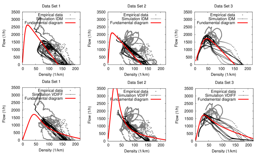
Figure 2: Microscopic flow-density relations $(Q(t),\rho(t))$ derived from the given and simulated gaps $s(t)$ and velocities $v(t)$, respectively. In addition, the equilibrium flow-density relations (fundamental diagrams) are plotted as well. This representation offers an alternative view to Fig. 1 on the empirical and simulated data, in particular with respect to traffic stability.

Sensitivity Analysis

Starting from the optimized model parameters summarized in Table 1, it is straightforward to vary a single model parameter while keeping the other parameters constant. The resulting one-dimensional scan of the parameter space gives a good insight in the model’s parameter properties and sensitivity. Furthermore, the application of different objective functions such as (7), (9) and (10) can be seen as a benchmark for the robustness of the model calibration. A “good” model should not strongly depend on the chosen error measure.

Figure 3 shows the resulting error measures of dataset 3. Remarkably, all error curves for the IDM are smooth and show only one minimum (which is therefore easy to determine by the optimization algorithm). As the datasets mainly describe car-following situations in obstructed traffic and standstills, the IDM parameters $T$, $s_{0}$ and $a$ are particularly significant and show distinct minima for the three proposed error measures while the values of $v_{0}$ were hard to determine exactly from the datasets 1 and 2 where the desired velocity is never approximated. The comfortable deceleration $b$ is also not very distinct (not shown here). The solutions belonging to different objective functions are altogether in the same parameter range. This robustness of the IDM parameter space is an important finding of this study.

The results for the VDIFF imply a less positive model assessment: The calibration results strongly vary with the chosen objective function indicating a strong sensitivity of the model parameters. Furthermore, too high values of the desired velocity lead to vehicle collisions in the simulation as indicated by an abrupt raise in the error curves. Interestingly, the sensitivity parameter $\lambda$ (taking into account velocity differences) has to be larger than approximately 0.5 in order to avoid accidents. Velocity differences are therefore a crucial input quantity for car-following models.

Figure 3: Systematic variation of one model parameter while keeping the other parameters at the optimal values listed in Table 1. The diagrams show the considered error measures (7), (9) and (10) for the IDM (left column) and VDIFF (right column) using dataset 3. The errors are plotted in logarithmic scale.

Consideration of an Explicit Reaction Time

The considered car-following models describe an instantaneous reaction (in the acceleration) to the leading car. A complex reaction time is, however, an essential feature of human driving due to physiological aspects of sensing, perceiving, deciding, and performing an action. Therefore, it is interesting to incorporate a reaction time in the IDM and the VDIFF and to investigate whether an additional model parameter will improve the calibration results.

A reaction time $T_{r}$ can be additionally incorporated in a time-continuous model of the type (1) by evaluating the right-hand side at a previous time $t-T_{r}$. If the reaction time is a multiple of the update time interval, $T_{r}=n\Delta t$, it is straightforward to consider all input quantities at $n$ time steps in the past. If $T_{r}$ is not a multiple of the update time interval $\Delta t$, we use a linear interpolation proposed in Ref. [14] according to

$$x(t-T_{r})=\beta x_{t-n-1}+(1-\beta)x_{t-n},$$ (14)

where $x$ denotes any input quantity such as $s$, $v$ or $\Delta v$ (cf. the right-hand side of Eq. (1)) and $x_{t-n}$ denotes this quantity taken $n$ time steps before the actual step. Here, $n$ is the integer part of $T_{r}/\Delta t$, and the weight factor of the linear interpolation is given by $\beta=T_{r}/\Delta t-n$. As initial conditions, values for the dependent variables are required for a whole time interval $T_{r}$. In the simulations, we used as initial conditions the values from the empirical data. For the stability properties of the IDM with reaction time, we refer to Ref. [13].

Figure 4 shows the systematic variation of the reaction time $T_{r}$ while keeping the other parameters at their optimal values as listed in Table 1 for the mixed error measure (10). Interestingly, an additional reaction time $T_{r}$ does not decrease the fit errors. Moreover, for small reaction times, there is no influence at all while values larger than a critical reaction time cause collisions as indicated by the abrupt raise in the errors. For the IDM, this critical reaction time $T_{c}^{\text{crit}}$ is smaller but of the order of the calibrated time gap parameters for the three sets. Similar values have been found for the VDIFF. As the VDIFF does not feature an explicit time gap parameter, however, it is not so easy to interpret.

The reason for the relatively high values of $T_{c}^{\text{crit}}$ is that the considered scenarios are limited to a single pair of vehicles over a limited duration and therefore only local stability properties can be tested. This finding is in agreement with a simulation study on local and collective stability properties of the IDM with explicit delay [13, 15]. Furthermore, the negligible influence of the reaction time as an explanatory variable can be interpreted in the way that the human drivers are able to compensate for their considerable reaction time (which is about 1 s [16]) by anticipation due to their driving experience. These compensating influences have recently been modeled and analyzed in [14, 13].

Figure 4: Systematic variation of a reaction time which has been explicitly incorporated in the Intelligent Driver Model (IDM) and the Velocity Difference Model (VDIFF). The reaction time $T_{r}$ has only a small influence for values well below the time gap $T$ which is an explicit model parameter of the IDM but only implicitly implemented in the VDIFF. Higher reaction times lead to collisions resulting in rapidly growing errors due to numerical penalties.

Validation by Cross-Comparison

Let us finally validate the obtained calibrated parameters by applying these settings to the other datasets, i.e., using the parameters calibrated on the basis of another dataset. We use the three optimal parameter settings listed in Table 1 and restrict ourselves to the mixed error measure (10). The obtained errors can be found in Table 2.

This cross-comparison allows to check for the reliability of the obtained parameters and automatically takes into account the variance of the calibrated parameter values. For the IDM, the obtained errors for the cross-compared simulation runs are of the same order as for the calibrated parameter sets. Therefore, the car-following behavior of the IDM turned out to be robust with respect to reasonable changes of parameter settings. In contrast, the VDIFF is more sensitive leading to larger errors. One parameter set even led to collisions which is reflected in a huge error due to the applied crash penalty.

Model	Dataset	Calib. Set 1	Calib. Set 2	Calib. Set 3
IDM	Set 1	20.7%	28.8%	28.7%
	Set 2	35.2%	26.2%	40.1%
	Set 3	41.1%	27.0%	13.0%
VDIFF	Set 1	25.8%	64.3%	40.5%
	Set 2	28.8%	26.7%	39.6%
	Set 3	57.0%	3840%	19.0%%

Table 2: Cross-comparison of the calibrated parameters for the mixed error measure (10) by applying the calibrated parameter sets for the Intelligent Driver Model (IDM) and the Velocity Difference Model (VDIFF) to the other datasets. The underlined errors refer to the parameter values corresponding to the best calibration results.

Discussion and Conclusions

We have used the Intelligent Driver Model (IDM) and the Velocity Difference Model (VDIFF) to reproduce three empirical trajectories. We found that the calibration errors are between 11% and 30%. These results are consistent with typical error ranges obtained in previous studies [1, 2, 3]. Let us finally discuss three qualitative influences which contribute to these deviations between observation and reproduction. Note, however, that noise in the data contribute to the fit errors as well [17].

A significant part of the deviations between measured and simulated trajectories can be attributed to the inter-driver variability [18] as it has been shown by cross-comparison. Notice that microscopic traffic models can easily cope with this kind of heterogeneity because different parameter values can be attributed to each individual driver-vehicle unit. However, in order to obtain these distributions of calibrated model parameters, more trajectories have to be analyzed, e.g., using the NGSIM trajectory data [19].

A second contribution to the overall calibration error results from a non-constant driving style of human drivers which is also referred to as intra-driver variability: Human drivers do not drive constantly over time, i.e., their behavioral driving parameters change. For a first estimation, we have compared the distances at standstills in the dataset 3 with the minimum distance as direct model parameter of the IDM. The driver stops three times because of red traffic lights. The bumper-to-bumper distances are $s_{\text{stop,1}}=1.39\,\mathrm{m}$, $s_{\text{stop,2}}=1.42\,\mathrm{m}$ and $s_{\text{stop,3}}=1.64\,\mathrm{m}$. These different values in similar situations already indicate that a deterministic car-following model allows only for an averaged and, thus, “effective” description of the human driving behavior resulting in parameter values that capture the “mean” observed driving performance. Considering the theoretical “best case” of a perfect agreement between data and simulation for all times except for the three standstills, the relative error function depends on $s_{0}$ only and an analytical minimization of $s_{0}$ results in $s_{0}^{\text{opt}}\approx 1.458\,\mathrm{m}$. This optimal solution defines a theoretical lower bound (based on about $15\%$ of the data of the considered time series) for the relative error measure of $\xi_{\text{min}}(s_{0}^{\text{opt}})\approx 7.9\%$. Therefore, the intra-driver variability accounts for a large part of the deviations between simulations and empirical observations. This influence could be captured by considering time-dependent model parameters reflecting driver adaptation processes as for example proposed in [20, 21].

Finally, driver anticipation contributes to the overall error as well but is not incorporated in simple car-following models. This is one possible cause for a model error, i.e., the residual difference between a perfectly time-independent driving style and a model calibrated to it. For example, we found a negligible influence of the additionally incorporated reaction time indicating that human drivers very well anticipate while driving and therefore compensate for their physiological reaction time. However, these physiological and psychological aspects can only be determined indirectly by looking at the resulting driving behavior. Consequently, it would be interesting to check if a negative “reaction” (or rather “anticipation”) time decreases the calibration errors. More complex microscopic traffic models try to take those aspects into account [14]. Note, however, that multi-leader anticipation requires trajectory data because the data recording using radar sensors of single “floating” cars is limited to the immediate predecessor [22].

Acknowledgment: We thank Dirk Helbing for a thorough review of the manuscript and fruitful discussion.

References

- [1] E. Brockfeld, R. D. Kühne, and P. Wagner, “Calibration and validation of microscopic traffic flow models,” Transportation Research Record 1876, 62–70 (2004).
- [2] P. Ranjitkar, T. Nakatsuji, and M. Asano, “Performance evaluation of microscopic flow models with test track data,” Transportation Research Record 1876, 90–100 (2004).
- [3] V. Punzo and F. Simonelli, “Analysis and comparision of microscopic flow models with real traffic microscopic data,” Transportation Research Record 1934, 53–63 (2005).
- [4] S. Ossen and S. P. Hoogendoorn, “Car-following behavior analysis from microscopic trajectory data,” Transportation Research Record 1934, 13–21 (2005).
- [5] S. Hoogendoorn, S. Ossen, and M. Schreuder, “Adaptive Car-Following Behavior Identification by Unscented Particle Filtering,” in Adaptive Car-Following Behavior Identification by Unscented Particle Filtering (Transportation Research Board Annual Meeting, Washington, D.C., 2007), paper number: 07-0950.
- [6] Deutsches Zentrum für Luft- und Raumfahrt (DLR), “Clearing house for transport data and transport models,”, http://www.dlr.de/cs/ – Access date: May 5, 2007.
- [7] M. E. Fouladvand and A. H. Darooneh, “Statistical analysis of floating-car data: an empirical study,” The European Physical Journal B 47, 319–328 (2005).
- [8] S. Panwai and H. Dia, “Comparative evaluation of microscopic car-following behavior,” IEEE Transactions on Intelligent Transportation Systems 6, 314–325 (2005).
- [9] M. Treiber, A. Hennecke, and D. Helbing, “Congested traffic states in empirical observations and microscopic simulations,” Physical Review E 62, 1805–1824 (2000).
- [10] R. Jiang, Q. Wu, and Z. Zhu, “Full velocity difference model for a car-following theory,” Physical Review E 64, 017101 (2001).
- [11] M. Bando, K. Hasebe, A. Nakayama, A. Shibata, and Y. Sugiyama, “Dynamical model of traffic congestion and numerical simulation,” Physical Review E 51, 1035–1042 (1995).
- [12] D. E. Goldberg, Genetic algorithms in search, optimization, and machine learning (Addision-Wesley, 1989).
- [13] A. Kesting and M. Treiber, “How reaction time, update time and adaptation time influence the stability of traffic flow,” Computer-Aided Civil and Infrastructure Engineering 23, 125–137 (2008).
- [14] M. Treiber, A. Kesting, and D. Helbing, “Delays, inaccuracies and anticipation in microscopic traffic models,” Physica A 360, 71–88 (2006).
- [15] M. Treiber, A. Kesting, and D. Helbing, “Influence of reaction times and anticipation on the stability of vehicular traffic flow,” Transportation Research Record 1999, 23–29 (2007).
- [16] M. Green, “”How long does it take to stop?” Methodological analysis of driver perception-brake times,” Transportation Human Factors 2, 195–216 (2000).
- [17] S. Ossen and S. P. Hoogendoorn, “Validity of Trajectory-Based Calibration Approach of Car-Following Models in the Presence of Measurement Errors,” Transportation Research Record (2008), in print.
- [18] S. Ossen, S. P. Hoogendoorn, and B. G. Gorte, “Inter-driver differences in car-following: A vehicle trajectory based study,” Transportation Research Record 1965, 121–129 (2007).
- [19] US Department of Transportation, “NGSIM – Next Generation Simulation,”, 2007, http://www.ngsim.fhwa.dot.gov – Access date: May 5, 2007.
- [20] M. Treiber and D. Helbing, “Memory effects in microscopic traffic models and wide scattering in flow-density data,” Physical Review E 68, 046119 (2003).
- [21] M. Treiber, A. Kesting, and D. Helbing, “Understanding widely scattered traffic flows, the capacity drop, and platoons as effects of variance-driven time gaps,” Physical Review E 74, 016123 (2006).
- [22] S. P. Hoogendoorn, S. Ossen, and M. Schreuer, “Empirics of Multianticipative Car-Following Behavior,” Transportation Research Record 1965, 112–120 (2006).