STATEFINDER DIAGNOSTIC FOR QUINTESSENCE WITH OR WITHOUT THERMAL INTERACTION

Abstract

The cosmological dynamics of minimally coupled scalar field that couples to the background matter with thermal interactions is investigated by using statefinder diagnostics. The time evolution of the statefinder pairs $\{r,s\}$ and $\{r,q\}$ are obtained under the circumstance that different values of model parameters are chosen. We show that the thermal coupling term does not affect the location of the late-time attractor, but exert an influence on the evolution of the statefinder parameters. The most notable feature of the $r-s$ plane for the thermal coupling model which is distinguished from the other dark energy models is that some part of the curve with thermal coupling can form a closed loop in the second quadrant ($r>1,s<0$).

1 Introduction

Various of cosmological observations strongly suggest that our universe is undergoing an accelerated expansion phase. In order to explain the acceleration, an unexpected energy component of the cosmic budget, which dominate the universe only recently, is introduced by many cosmologists. However, the physical origin of dark energy is still mysterious.

Perhaps the simplest proposal is the Einstein’s cosmological constant $\Lambda$ (vacuum energy), whose energy density remains constant with time. However, due to some conceptual problems associated with the cosmological constant (for a review, see [1, 2, 3]), a large variety of alternative possibilities have been explored. The most popular among them is quintessence scenario which uses a scalar field $\phi$ with a suitably chosen potential $V(\phi)$ so as to make the vacuum energy vary with time. A form of quintessence called ”tracker fields”, whose evolution is largely insensitive to initial conditions and at late times begin to dominate the universe with a negative equation of state, was introduced to avoids the problems relevant to cosmological constant [4]. Another approach to solve the puzzle is introducing an interaction term in the equations of motion, which describes the energy flow between the dark energy and the rest matter (mainly the dark matter) in the universe. It is found that, with the help of a suitable coupling, it is possible to reproduce any scaling solutions. Inclusion of a non-minimal coupling to gravity in quintessence models together with further generalization leads to models of dark energy in a scalar-tensor theory of gravity. Besides, some other models invoke unusual material in the universe such as Chaplygin gas, tachyon, phantom or k-essence (see, for a review, [5] and reference therein).

As so many dark energy models have been proposed, it becomes urgent to give them an unambiguous discrimination. The equation of state $w$, could discriminate some basic dark energy models properly, for example, $w=-1$ for cosmological constant, $w>-1$ for quintessence and $w<-1$ for phantom, but as more and more interacting models were investigated, the ambit of $w$ become not so clear. A new geometrical diagnostic, dubbed the statefinder pair $\{r,s\}$ is proposed by Sahni et al [6], where $r$ is only determined by the scalar factor $a$ and its derivatives with respect to the cosmic time $t$, just as the Hubble parameter $H$ and the deceleration parameter $q$, and $s$ is a simple combination of $r$ and $q$. The statefinder pair has been used to explor a series of dark energy and cosmological models [7, 8, 9, 10]. As is analyzed, the ”distance” from a given dark energy model to the LCDM scenario can be clearly identified via the $r(s)$ evolution diagram. The current values of $r$ and $s$, which can be calculated in models, are evidently valuable since it is expected that they can be extracted from data coming from SNAP (SuperNovae Acceleration Probe) type experiments. Therefore, the statefinder diagnostic combined with future observations may possibly be used to discriminate between different dark energy models [8, 9].

The effects of thermal coupling between the quintessence field and the ordinary matter particles was first investigated by Hsu and Murray [11]. They set the quintessence field to be a static external source for a Euclidean path integral depicting the thermal degree of freedom and let the time-like boundary conditions of the path integral have a period which is decided by the inverse of temperature. And they show that if in the early universe matter particles are in thermal equilibrium, quantum gravity [12] will induce an effective thermal mass term for quintessence field $\phi$, which takes the form

$$\left(\frac{\beta}{M_{P}}\right)^{2}\phi^{2}T^{4},$$ (1)

where $T\propto a^{-1}$ denotes a measurement of temperature of background matter, $M_{P}$ the Planck mass scale, $\beta$ a dimensionless constant, $a$ the scale factor (with current value $a_{0}=1$), and find that even Planck-suppressed interactions between matter and the quintessence field can alter its evolution qualitatively. In a previous paper [13], we investigated the dynamics of the cosmology with quintessence using the phase space analysis, which has the above thermal coupling to the matter in a complete manner and analyzed the conditions for the existence and stability of various critical points as well as their cosmological implications. In this paper, we apply the statefinder diagnostic to the cosmological dynamics of minimally coupled scalar field that couples to the background matter with thermal interactions.

2 The Setup

Let us study quintessence with thermal coupling to ordinary matter particles in spatially flat FRW cosmological background

$$ds^{2}=dt^{2}-a^{2}(t)d\textbf{x}^{2}.$$ (2)

For the spatially homogeneous scalar field minimally coupled to gravity with thermal interaction (1), the evolution is governed by the Klein-Gordon equation

$$\ddot{\phi}+3H\dot{\phi}+V^{\prime}(\phi)=2\left(\frac{\beta}{M_{P}}\right)^{2}\phi T^{4},$$ (3)

where the overdots denote the derivative with respect to cosmic time and the prime denotes the derivative with respect to $\phi$. Here the Hubble parameter $H\equiv\dot{a}/a$ is determined by the Friedmann equation

$$H^{2}=\frac{\kappa^{2}}{3}\left[\rho_{m}+\frac{1}{2}\dot{\phi}^{2}+V(\phi)\right]$$ (4)

and

$$\dot{H}=-\frac{\kappa^{2}}{2}(\rho_{m}+p_{m}+\dot{\phi}^{2}),$$ (5)

where $\kappa^{2}\equiv 8\pi/M_{p}^{2}$, $\rho_{m}$ and $p_{m}$ are the energy density and pressure of the baryotropic matter, respectively. From Eqs.(3)-(5) and the conservation of energy, $\rho_{m}$ satisfies the following continuous equation

$$\dot{\rho_{m}}+3H(\rho_{m}+p_{m})=-2\left(\frac{\beta}{M_{P}}\right)^{2}\phi\dot{\phi}T^{4},$$ (6)

and $p_{m}=(\gamma-1)\rho_{m}$, where $\gamma$ is a constant, $0\leq\gamma\leq 2$, such as radiation($\gamma=4/3$) or dust ($\gamma=1$). It is clear that when the thermal coupling parameter $\beta$ becomes zero, the equations (3)-(6) will return to those of the standard one scalar field quintessence scenario. In current situation, both quintessence and baryotropic matter are not conserved, but the conservation of the overall energy holds.

To be concrete, in this paper we only consider the quintessence with an exponential potential energy density, i.e.,

$$V(\phi)=V_{0}\exp(-\lambda_{0}\kappa\phi)$$ (7)

where the parameter $V_{0}$ and $\lambda_{0}$ are two positive constants. Exponential potentials have been studied extensively in various situations, and these are of interest for two main reasons. Firstly, they can be derived from a good candidate of fundamental theory for such being string/M theory; secondly, the equations of motion can be written as an autonomous system in the situation.

Introducing the following dimensionless variables:

$$x=\frac{\kappa\dot{\phi}}{\sqrt{6}H},\;\;y=\frac{\kappa\sqrt{V(\phi)}}{\sqrt{3}H},\;\;z=\frac{\kappa}{M_{p}}\frac{\phi}{\sqrt{3}a^{2}H},\;\;\xi=\frac{\sqrt{6}}{\kappa\phi},\;\;N=\ln a$$ (8)

and taking the potential (7) into account, we can rewrite the equation system (4)-(6) as the following autonomous system:

$$\frac{dx}{dN} = \frac{3}{2}x[\gamma(1-x^{2}-y^{2})+2x^{2}]-(3x+\beta^{2}z^{2}\xi-\frac{1}{2}\lambda_{0}y^{2}),$$

$$\frac{dy}{dN} = \frac{3}{2}y[\gamma(1-x^{2}-y^{2})+2x^{2}]-\frac{1}{2}\lambda_{0}xy,$$

$$\frac{dz}{dN} = \frac{3}{2}z[\gamma(1-x^{2}-y^{2})+2x^{2}]-2z+xz\xi,$$

$$\frac{d\xi}{dN} = -x\xi^{2}.$$ (9)

3 Statefinder Parameters

The traditional geometrical diagnostics, i.e., the Hubble parameter $H$ and the deceleration parameter $q\equiv{-\ddot{a}a}/{\dot{a}^{2}}$, are two good choices to describe the expansion state of our universe but they can not characterize the cosmological models uniquely, because a quite number of models may just correspond to the same current value of $H$ and $q$. Fortunately, as is shown in many literatures, the statefinder pair $\{r,s\}$ which is also a geometrical diagnostic, is able to distinguish a series of cosmological models successfully.

The statefinder pair $\{r,s\}$ defines two new cosmological parameters in addition to $H$ and $q$:

$$r\equiv\frac{1}{aH^{3}}\frac{d^{3}a}{dt^{3}},\;\;\;\;s\equiv\frac{r-1}{3(q-1/2)}.$$ (10)

As an important function, the statefinder can allow us to differentiate between a given dark energy model and the simplest of all models, i.e., the cosmological constant $\Lambda$. For the $\Lambda$CDM model, the statefinder diagnostic pair $\{r,s\}$ takes the constant value $\{1,0\}$, and for the SCDM model, $\{1,1\}$.

From Eqs. (10) and (8), the statefinder parameter $r$ can be explicitly written as

$$r=1+\frac{9}{2}\gamma(\gamma-1)(1-x^{2}-y^{2})+3(\gamma-2)\beta^{2}xz^{2}\xi+9x^{2}-3\lambda_{0}xy.$$ (11)

And the deceleration parameter $q$ is given by

$$q=\frac{3}{2}\gamma(1-x^{2}-y^{2})+3x^{2}-1.$$ (12)

Therefore, the other statefinder parameter $s$ is equal to

$$s=\frac{\gamma(\gamma-1)(1-x^{2}-y^{2})+\frac{2}{3}(\gamma-2)\beta^{2}xz^{2}\xi+2x^{2}-\frac{2}{3}\lambda_{0}xy}{\gamma(1-x^{2}-y^{2})+2x^{2}-1}.$$ (13)

We draw a $\gamma-\lambda^{2}$ plane in Figure 1 and divide it into different regions. From the analysis of our previous paper [13], we know that the equation system, Eqs.(2), have a sole late-time attractor only if the conditions $\gamma<4/3$ and/or $\lambda_{0}^{2}<24$ are satisfied. It is easy to find that these conditions correspond to region A and B in Figure 1 and the common boundary of region A and B is the segment of straight line $\lambda_{0}^{2}=18\gamma$. In what follows, we call the condition that region A satisfies case A and that region B satisfies case B. For case A and case B, the attractor $(x_{c},y_{c},z_{c},\xi_{c})$ is located at the point $(\lambda_{0}/6,\sqrt{36-\lambda_{0}^{2}}/6,0,0)$ and $(3\gamma/\lambda_{0},3\sqrt{\gamma(2-\gamma)}/\lambda_{0},0,0)$ in the phase space, respectively. It is readily to check that in the common boundary of region A and B, there actually exists only one attractor as is expected. It is also worth pointing out that the attractor depends only on the parameter $\lambda$ for case A, and for both cases, the attractor has nothing to do with the coupling parameter $\beta$. In statefinder parameter space, the attractor lies at the point $(r_{c},q_{c},s_{c})$ and it can be expressed explicitly by

$$r_{c} = 1+\frac{\lambda_{0}^{2}}{12}\left(3-\sqrt{36-\lambda_{0}^{2}}\right),\;\;$$

$$q_{c} = -1+\frac{\lambda_{0}^{2}}{12},\;\;$$

$$s_{c} = \frac{{\lambda_{0}^{2}}\left(3-\sqrt{36-\lambda_{0}^{2}}\right)}{3\left(\lambda_{0}^{2}-18\right)}$$ (14)

for case A and

$$r_{c} = 1+\frac{9}{2}\gamma(\gamma-1)+\frac{81(\gamma-2)\gamma^{2}}{\lambda_{0}^{2}}-\frac{27\gamma\sqrt{(2-\gamma)\gamma}}{\lambda_{0}},$$

$$q_{c} = -1+\frac{3\gamma}{2},$$

$$s_{c} = \gamma+\frac{18(\gamma-2)\gamma^{2}}{(1-\gamma)\lambda_{0}^{2}}+\frac{6\gamma\sqrt{(2-\gamma)\gamma}}{(1-\gamma)\lambda_{0}}$$ (15)

for case B, respectively.

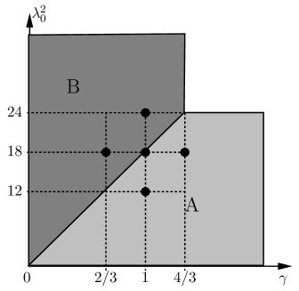
Figure 1: The schematic illustration of the parameter space. In region A and B, the autonomous system (2) has a late-time attractor, respectively.

Let us now turn to statefinder parameters plane analysis. We shall investigate the properties of the evolution trajectories of statefinder parameters with three parameters $\beta$, $\gamma$ and $\lambda_{0}$, by fixing two of them and varying the rest. Note that we are only interested in case A and case B, due to the existence of the attractor solution.

We first fix the brayotropic parameter $\gamma$ and potential parameter $\lambda_{0}$, and let the thermal coupling constant $\beta$ be adjustable. We show the time evolution of the statefinder pairs $\{r,s\}$ (left panels) and $\{r,q\}$ (right panels) in Figure 2, Figure 3 and Figure 4 where the fixed parameters $\gamma=1$ and $\lambda_{0}=1,4,7$, respectively. In these three figures, we choose an initial state that the universe was ongoing a decreasing expansion and the kinetic energy of the quintessence is negligible. The trajectories plotted in Figure 2 and Figure 3 correspond to case A. Obviously, they are all located in the second ($s<0,r>1$) and/or fourth ($s>0,r<1$) quadrants in the $r-s$ plane. This is not surprising because we have assumed that the equation of state of quintessence field became negative after some past moment and this makes the deceleration parameter $q<1/2$ from then on as is shown in right panels of Figure 2 and Figure 3. From the definition of statefinder parameter $s$, Eq.(10), it is easy to find that if $r<1$ then $s>0$, if $r>1$ then $s<0$ and if $r=1$ and $q\neq 1/2$ then $s=0$ which is just corresponding to the $\Lambda$CDM fixed point. It is worth pointing out that the attractors in the two figures have different cosmological implication: the attractor illustrated in Figure 2 means eternal acceleration of the universe, while the one in Figure 3 means the universe will decelerate in the future. The trajectories plotted in Figure 4 correspond to case B. The accelerating rate of expansion of the universe will be determined only by the baryotropic matter. We choose the baryotropic parameter $\gamma=1$ in Figure 4 which means the universe will be decelerated in the future, as is shown in the $r-q$ plane (right panel). From these three figures, we see that the thermal coupling term enhances the possible maximum value of $r$ and makes it first increase to a maximum value ($>1$) then decrease. This effect reflected in the $r-s$ plane is that some parts of the $\beta\neq 0$ curves can be located in the second quadrants ($r>1,s<0$) and these parts form closed loops. This feature of the $r-s$ plane for the thermal interacting quintessence model is distinguished from those of ordinary quintessence and other dark energy models.

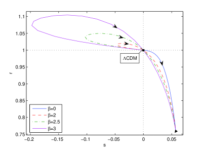
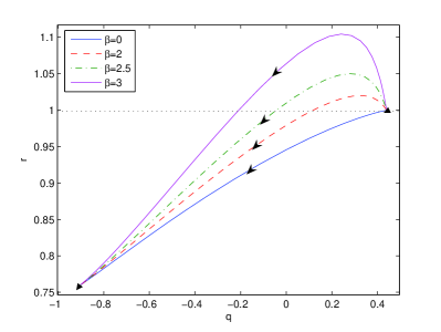
Figure 2: The time evolution of the statefinder pairs $\{r,s\}$ and $\{r,q\}$ is illustrated in left and right panel, respectively. In both panels the model parameter $\gamma$ and $\lambda_{0}$ are fixed to be unity and the thermal coupling constant $\beta$ takes different values. For $\beta=0$ curve, $r$ and $s$ monotonically decrease from $1$ and increase from $0$ to the value the attractor takes, respectively, and $q$ also monotonically decrease from positive to negative. For $\beta\neq 0$ curves, $q$ keeps monotonically decreasing, whereas $r$ ($s$) first increase (decrease) from $1$ ($0$) to a maximum (minimum) value then decrease (increase) and pass through the $\Lambda$CDM fixed point (in $r-s$ plane) to the attractor.

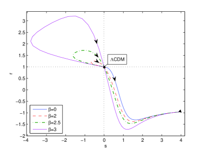
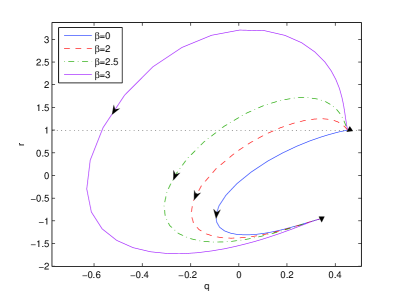
Figure 3: The time evolution of the statefinder pairs $\{r,s\}$ and $\{r,q\}$ is illustrated in left and right panel, respectively. Here the fixed model parameters are chosen to be $\gamma=1$ and $\lambda_{0}=4$, whereas the thermal coupling constant $\beta$ takes different values. For $\beta=0$ curve, $s$ monotonically increase from $0$ to the value the attractor takes, while $r$ and $q$ first decrease from the start point to a minimum value then increase to the attractor. For $\beta\neq 0$ curves, $q$ has the similar behavior of that of $\beta=0$ curve, whereas $r$ ($s$) first increase (decrease) from $1$ ($0$) to a maximum (minimum) value then decrease (increase) and after passing through the $\Lambda$CDM fixed point (in $r-s$ plane), they show a similar behavior of that of $\beta=0$ curve.

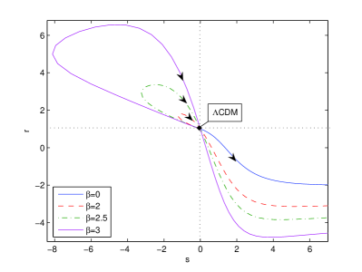
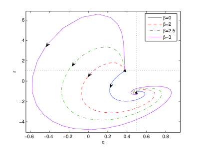
Figure 4: The time evolution of the statefinder pairs $\{r,s\}$ and $\{r,q\}$ is illustrated in left and right panel, respectively. Here the fixed model parameters are chosen to be $\gamma=1$ and $\lambda_{0}=7$, while the thermal coupling constant $\beta$ takes different values. Because $q$ approaches to and takes the value of $1/2$ many times at the late time, but at the same time $r$ is always less than unity, the value of $s$ will become infinity many times. Therefore, the plot in the left panel shows only a piece of the whole time evolution.

Next, let us show the dependence of the time evolution of the statefinder pair $\{r,s\}$ on the brayotropic parameter $\gamma$ and potential parameter $\lambda_{0}$ in the absence or presence of the thermal interaction. In Figure 5, without loss of generality the brayotropic parameter $\gamma$ is fixed to be unity and the potential parameter is selected to satisfy the condition $\lambda_{0}^{2}=12,18,24$, respectively. The left panel shows the evolution for the case that thermal interaction is absent ($\beta=0$) and the right one for the case with thermal interaction (we set $\beta=4$ here for example).Clearly, the effect that the thermal coupling term exerts is the same as that pointed out previously. The $\lambda_{0}^{2}=12$ curve has a definite end point which locates the late-time attractor but the others haven’t. This is not surprising. The parameter related to the $\lambda_{0}^{2}=12$ curve lies in the region A of the parameter space (see Figure 1) and the location of the attractor is determined by Eqs. (3) which take definite values, while the parameters relevant to the other curves locate in the region B or the boundary line between region A and B, so the locations of the corresponding attractor is determined by Eqs. (3) which are infinite for the parameters selected. The situation is similar in Figure 6, where we fix the value of $\lambda$ and select three different representative values for $\gamma$. In addition, the dark dots marked on the curves in the two figures represent the present values of the statefinder parameters $\{r_{0},s_{0}\}$. It should be noted that the true values of $\{r_{0},s_{0}\}$ of the universe should be determined in a model-independent way, which we can only place our hope on the future experiments. In principle, if this is achieved, the statefinder parameters can be viewed as a discriminator for testing various cosmological models.

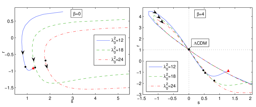
Figure 5: The trajectories in the statefinder plane $\{r,s\}$ for the model where we fix the baryotropic parameter $\gamma$ to be unity and let the thermal coupling constant $\beta=0$ and $\beta=4$ in the left and right panel, respectively. The dark dots indicate the current value of statefinder parameters. The triangle at the end of the $\lambda_{0}^{2}=12$ curve denotes the location of the late-time attractor. For the other two curves the attractor is located at infinity.

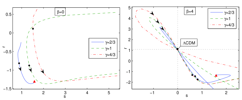
Figure 6: The trajectories in the statefinder plane $\{r,s\}$ for the model where we fix the baryotropic parameter $\lambda_{0}=\sqrt{18}$ and let the thermal coupling constant $\beta=0$ and $\beta=4$ in the left and right panel, respectively. The dark dots indicate the current value of statefinder parameters. The triangle at the end of the $\gamma=2/3$ curve denotes the location of the late-time attractor. For the other two curves the attractor is located at infinity.

4 Conclusions

We have investigated the time evolution of quintessence field with an exponential potential and with or without thermal coupling to the background matter in a flat FRW universe from the statefinder viewpoint in this paper. The statefinder diagnostic have been performed. It is found that that the thermal coupling term does not affect the location of the late-time attractor which is determined only by the potential of the quintessence field and the background baryotropic matter, but exert an influence on the evolution of the statefinder parameters. The most notable feature for the thermal coupling model which is distinguished from the other dark energy models is that the curve with thermal coupling can form a closed loop in the second quadrant ($r>1,s<0$) in the $r-s$ plane. What we expect now is that more and more accurate observational data could be offered to determine the model parameters more and more precisely, rule out some models and consequently shed light on the essence of dark energy.

References

- [1] S. Weinberg, Rev. Mod. Phys. 61 (1989) 1.
- [2] V. Sahni and A. A. Starobinsky, Int. J. Mod. Phys. D9 (2000) 373 [astro-ph/9904398].
- [3] T. Padmanabhan, Phy. Rep. 380 (2003) 235 [hep-th/0212290].
- [4] I. Zlatev, L. Wang and P. J. Steinhardt, Phys. Rev. Lett. 82 (1999) 896 [astro-ph/9807002].
- [5] E. J. Copeland, M. Sami and S. Tsujikawa, Int. J. Mod. Phys. D15 (2006) 1753 [hep-th/0603057].
- [6] V. Sahni, T. D. Saini, A. A. Starobinsky and U. Alam, JETP Lett. 77 (2003) 201 [astro-ph/0201498].
- [7] U. Alam, V. Sahni, T. D. Saini and A. A. Starobinsky, Mon. Not. Roy. Astron. Soc. 344 (2003) 1057 [astro-ph/0303009].
- [8] X. Zhang, Phys. Lett. B611 (2005) 1 [astro-ph/0503075].
- [9] X. Zhang, Int.J. Mod. Phys. D14 (2005) 1597 [astro-ph/0504586].
-
[10]
W. Zimdahl, D. Pavon, Gen. Rel. Grav. 36 (2004) 1483 [gr-qc/0311067];
P. X. Wu, H. W. Yu, Int. J. Mod. Phys. D14 (2005) 1873 [gr-qc/0509036];
B. Chang, et al., JCAP 0701 (2007) 016 [astro-ph/0612616];
M. R. Setare, J. Zhang and X. Zhang, JCAP 0703 (2007) 007 [gr-qc/0611084];
J. Zhang, X. Zhang and H. Liu, Phys. Lett. B659 (2008) 26 [arXiv:0705.4145[astro-ph]];
Z.-L. Yi and T.-J. Zhang, Phys. Rev. D75 (2007) 083515 [astro-ph/0703630];
H. Wei, R.-G. Cai, Phys. Lett. B655 (2007) 1 [arXiv:0707.4526 [gr-qc]];
D.-J. Liu, W.-Z. Liu, Phys. Rev. D77 (2008) 027301 [arXiv:0711.4854[astro-ph]];
W. Zhao, arXiv:0711.2319[gr-qc];
G. Panotopoulos, arXiv:0712.1177 [astro-ph]. - [11] S. Hsu and B. Murray, Phys. Lett. B595 (2004) 16 [astro-ph/0402541].
- [12] M. Kamionkowski and J. March-Russell, Phys. Lett. B282 (1992) 137 [hep-th/9202003].
- [13] D. -J. Liu and X. -Z. Li, Phys. Lett. B611 (2005) 8 [astro-ph/0501596].