Structure and Interpretation of Computer Programs

Abstract

Call graphs depict the static, caller-callee relation between “functions” in a program. With most source/target languages supporting functions as the primitive unit of composition, call graphs naturally form the fundamental control flow representation available to understand/develop software. They are also the substrate on which various interprocedural analyses are performed and are integral part of program comprehension/testing. Given their universality and usefulness, it is imperative to ask if call graphs exhibit any intrinsic graph theoretic features – across versions, program domains and source languages. This work is an attempt to answer these questions: we present and investigate a set of meaningful graph measures that help us understand call graphs better; we establish how these measures correlate, if any, across different languages and program domains; we also assess the overall, language independent software quality by suitably interpreting these measures.

1 Introduction

Complexity is one of the most pertinent characteristics of computer programs and, thanks to Moore’s law, computer programs are becoming ever larger and complex; it’s not atypical for a software product to contain hundreds of thousands, even millions of lines of code where individual components interact in myriad of ways. In order to tackle such complexity, variety of code organizing motifs were proposed. Of these motifs, functions form the most fundamental unit of source code: software is organized as set of functions – of varying granularity and utility, with functions computing various results on their arguments. Critical feature of this organizing principle is that functions themselves can call other functions. This naturally leads to the notion of function call graph where individual functions are nodes, with edges representing caller-callee relations; indegree depicts the number of functions that could call the function and outdegree depicts the number of functions that this function can call. Since no further restrictions are employed, the caller-callee relation induces a generic graph structure, possibly with loops and cycles.

In this work we study the topology of such (static) call graphs. Our present understanding of call graphs is limited; we know: that call graphs are directed and sparse; can have cycles and often do; are not strongly connected; evolve over time and could exhibit preferential attachment of nodes and edges. Apart from these basic understanding, we do not know much about the topology of call graphs.

2 Contributions

In this paper we answer questions pertaining to topological properties of call graphs by studying a representative set of open-source programs. In particular, we ask following questions: What is the structure of call graphs? Are there any consistent properties? Are some properties inherent to certain programming language/problem class? In order to answer these questions, we investigate set of meaningful metrics from plethora of graph properties [9]. Our specific contributions are:

1) We motivate and provide insights as to why certain call graph properties are useful and how they could help us develop better and robust software. 2) We compare graph structure induced by different language paradigms under an eventual but structurally immediate structure – call graphs. The authors are unaware of any study that systematically compare the call graphs of different languages; in particular, the “call graph” structure of functional languages. 3) Our corpus, being varied and large, is far more statistically representative compared to the similar studies ([24], [4],[18]). 4) We, apart from confirming previous results in a rigorous manner, also compute new metrics to capture finer aspects of graph structure. 5) As a side effect, we provide a potential means to assess software quality, independent of the source language.

Rest of the paper is organized as follows. We begin by justifying the utility of our study and proceed to introduce relevant structural measures in section 4. Section 5 discusses the corpus and methodology. We then present our the measurements and interpretations (Section 6). We conclude with section 7 and 8.

3 Motivation

Call graphs define the set of permissible interactions and information flows and could influence software processes in non trivial ways. In order to give the reader an intuitive understanding as to how graph topology could influence software processes, we present following four scenarios where it does.

Bug Propagation Dynamics Consider how a bug in some function affects the rest of the software. Let foo call bar and bar could return an incorrect value because of a bug in bar. if foo is to incorporate this return value in its part of computation, it is likely to compute wrong answer as well; that is, bar has infected foo. Note that such an infection is contagious and, in principle, bar can infect any arbitrary function $f_{n}$ as long as $f_{n}$ is connected to bar. Thus connectedness as graph property trivially translates to infectability. Indeed, with appropriate notions of infection propagation and immunization, one could understand bug expression as an epidemic process. It is well known that graph topology could influence the stationary distribution of this process. In particular, the critical infection rate – the infection rate beyond which an infection is not containable – is highly network specific; in fact, certain networks are known to have zero critical thresholds [5]. It pays to know if call graphs are instances of such graphs.

Software Testing: Different functions contribute differently to software stability. Certain functions that, when buggy, are likely to render the system unusable. Such functions, functions whose correctness is central to statistical correctness of the software, are traditionally characterized by per-function attributes like indegree and size. Such simple measure(s), though useful, fail to capture the transitive dependencies that could render even a not-so-well connected function an Achilles heel. Having unambiguous metrics that measure a node’s importance helps making software testing more efficient. Centrality is such a measure that gives a node’s importance in a graph. Once relevant centrality measures were assigned, one could expend relatively more time testing central functions. Or, equally, test central functions and their called contexts for prevalent error modes like interface nonconformity, context disparity and the likes ([21], [7]). By considering node centralities, one could bias the testing effort to achieve similar confidence levels without a costlier uniform/random testing schedule; though most developers intuitively know the importance of individual functions and devise elaborate test cases to stress these functions accordingly, we believe such an idiosyncratic methodology could be safely replaced by an informed and statistically tenable biasing based on centralities. Centrality is also readily helpful in software impact analysis.

Software Comprehension: Understanding call graph structure helps us to construct tools that assist the developers in comprehending software better. For instance, consider a tool that magically extracts higher-level structures from program call graph by grouping related, lower-level functions. Such a tool, for example, when run on a kernel code base, would automatically decipher different logical subsystems, say, networking, filesystem, memory management or scheduling. Devising such a tool amounts to finding appropriate similarity metric(s) that partitions the graph so that nodes within a partition are “more” similar compared to nodes outside. Understandably, different notions of similarities entail different groupings. Recent studies show how network structure controls such grouping [2] and how per node graph metrics can be used to improve the developer-perceived clustering validity ([26], [17]).

Inter Procedural Analysis Call graph topology could influences both precision and convergence of Inter Procedural Analysis (IPA). When specializing individual procedures in a program, procedures that have large indegree could end up being less optimal: dataflow facts for these functions tend to be too conservative as they are required to be consistent across a large number of call sites. By specifically cloning nodes with large indegree and by distributing the indegrees “appropriately” between these clones, one could specialize individual clones better. Also, number of iterations an iterative IPA takes compute a fixed-point depends on the $max$(longest path length, largest cycle).

4 Statistical Properties of Interest

As with most nascent sciences, graph topology literature is strewn with notions that are overlapping, correlated and misused gratuitously; for clarity, we restrict ourselves to following structural notions. A note on usage: we employ graphs and networks interchangeably; $G=(V,E)$, $\mid V\mid=n$ and $\mid E\mid=m$; $(i,j)$ implies $i$ calls $j$; $d_{i}$ denotes the degree of vertex i and $d_{ij}$ denotes the geodesic distance between $i$ and $j$; $N(i)$ denotes the immediate neighbours of i; graphs are directed and simple: for every $(i_{1},j_{1})$ and $(i_{2},j_{2})$ present, either $(i_{1}\neq i_{2})$ or $(j_{1}\neq j_{2})$ is true.

Graphs, in general, could be modeled as random, small world, power-law, or scale rich, each permitting different dynamics.

Random graphs: random graph model [11], is perhaps the simplest network model: undirected edges are added at random between a fixed number $n$ of vertices to create a network in which each of the $\frac{1}{2}n(n-1)$ possible edges is independently present with some probability $p$, and the vertex degree distribution follows Poisson in the limit of large $n$.

Small world graphs: exhibit high degree of clustering and have mean geodesic distance $\ell$ – defined as, $\ell^{-1}=\frac{1}{n(n+1)}\sum_{i\neq j}d_{ij}^{-1}$ – in the range of $\log n$; that is, number of vertices within a distance $r$ of a typical central vertex grows exponentially with $r$ [19].

It should be noted that a large number of networks, including random networks, have $\ell$ in the range of $\log n$ or, even, $\log\log n$. In this work, we deem a network to be small world if $\ell$ grows sub logarithmically and the network exhibits high clustering.

Power law networks: These are networks whose degree distribution follow the discrete CDF: $P[X>x]\propto cx^{-\gamma}$ , where $c$ is a fixed constant, and $\gamma$ is the scaling exponent. When plotted as a double logarithmic plot, this CDF appears as a straight line of slope $-\gamma$. The sole response of power-law distributions to conditioning is a change in scale: for large values of $x$, $P[X>x|X>X_{i}]$ is identical to the (unconditional) distribution $P[X>x]$. This “scale invariance” of power-law distributions is attributed as scale-freeness. Note that this notion of scale-freeness does not depict the fractal-like self similarity in every scale.

Graphs with similar degree distributions differ widely in other structural aspects; rest of the definitions introduce metrics that permit finer classifications.

degree correlations: In many real-world graphs, the probability of attachment to the target vertex depends also on the degree of the source vertex: many networks show assortative mixing on their degrees, that is, a preference for high-degree nodes to attach to other high-degree node; others show disassortative mixing where high-degree nodes consistently attach to low-degree ones. Following measure, a variant of Pearson correlation coefficient [20], gives the degree correlation. $\rho=\frac{m^{-1}\sum_{i}j_{i}k_{i}-[m^{-1}\sum_{i}\frac{1}{2}(j_{i}+k_{i})]^{2}}{m^{-1}\sum_{i}\frac{1}{2}(j_{i}^{2}+k_{i}^{2})-[m^{-1}\sum_{i}\frac{1}{2}(j_{i}+k_{i})]^{2}}$ , where $j_{i}$, $k_{i}$ are the degrees of the vertices at the ends of $i^{th}$ edge, with $i=1\cdots m$. $\rho$ takes values in the range $-1\leq\rho\leq 1$, with $\rho>0$ signifying assortativity and $\rho<0$ signifying dissortativity. $\rho=0$ when there is no discernible correlation between degrees of nodes that share an edge.

scale free metric: a useful measure capturing the fractal nature of graphs is scale-free metric $s(g)$ [16], defined as: $s(g)=\sum_{(i,j)\in E}d_{i}d_{j}$ , along with its normalized variant $S(g)=\frac{s(g)}{s_{max}}$; $s_{max}$ is the maximal $s(g)$ and is dictated by the type of network understudy. Rest of the paper will use the normalized variant.

$s(g)$ is maximal when nodes with similar degree connect to each other [13]; thus, $S(g)$ is close to one for networks that are fractal like, where the connectivity, at all degrees, stays similar. On the other hand, in networks where nodes repeatedly connect to dissimilar nodes, $S(g)$ is close to zero. Networks that exhibit power-law, but have have a scale free metric $S(g)$ close to zero are called scale rich; power-law networks whose $S(g)$ value is close to one are called scale-free. Measures $S(g)$ and $\rho$ are similar and are correlated; but they employ different normalizations and are useful in discerning different features [16].

clustering coefficient: is a measure of how clustered, or locally structured, a graph is: it depicts how, on an average, interconnected each node’s neighbors are. Specifically, if node $v$ has $k_{v}$ immediate neighbors, then the clustering coefficient for that node, $C_{v}$, is the ratio of number of edges present between its neighbours $E_{v}$ to the total possible connections between $v$’s neighbours, that is, $k_{v}(k_{v}-1)/2$. The whole graph clustering coefficient, $C$, is the average of $C_{v}$s: that is, $C=\left<C_{v}\right>_{v}=\left<\frac{2E_{v}}{k_{v}(k_{v}-1)}\right>_{v}$.

clustering profile: $C$ has limited use when immediate connectivity is sparse. In order to understand interconnection profile of transitively connected neighbours, we use clustering profile [1]: $C^{d}_{k}=\frac{\sum_{\{i|d_{i}=k\}}C^{d}(i)}{|\{i|d_{i}=k\}|}$ , where $C^{d}(i)=\frac{|\{(j,k);j,k\in N(i)|{d_{jk}\in{G(V\setminus i)}}=d\}|}{{|N(i)|\choose 2}}$. Note that, by this definition, clustering coefficient $C$ is simply $C^{1}_{k}$,

centrality: of a node is a measure of relative importance of the node within the graph; central nodes are both points of opportunities – that they can reach/influence most nodes in the graph, and of constraints – that any perturbation in them is likely to have greater impact in a graph. Many centrality measures exist and have been successfully used in many contexts ([6], [10]). Here we focus on betweenness centrality $B_{u}$ (of node $u$), defined as the ratio of number of geodesic paths that pass through the node ($u$) to that of the total number of geodesic paths: that is, $B_{u}=\sum_{ij}\frac{\sigma(i,u,j)}{\sigma(i,j)}$; nodes that occur on many shortest paths between other vertices have higher betweenness than those that do not.

connected components: size and number of connected components gives us the macroscopic connectivity of the graph. In particular, number and size of strongly connected components gives us the extent of mutual recursion present in the software. Number of weakly connected component gives us the upper bound on amount of runtime indirection resolutions possible.

edge reciprocity: measures if the edges are reciprocal, that is, if $(i,j)\in E$, is $(j,i)$ also $\in E$? A robust measure for reciprocity is defined as [12]: $\rho=\frac{\varrho-\bar{a}}{1-\bar{a}}$ where $\varrho=\frac{\sum_{ij}a_{ij}a_{ji}}{m}$ and $\bar{a}$ is mean of values in adjacency matrix. This measure is absolute: $\rho$ greater than zero imply larger reciprocity than random networks and $\rho$ less than zero imply smaller reciprocity than random networks.

Figure 1: Indegree Distribution

5 Corpora & Methodology

We studied 35 open source projects. The projects are written in four languages: C, C++, OCaml and Haskel. Appendix Appendix I enlists these software, their source language, versiom, domain and size: number of nodes $N$ and the number of edges $M$. Most programs used are large, used by tens of thousands of users, written by hundreds of developers and were developed over years. These programs are actively developed and supported. Most of these programs – from proof assistant to media player, provide varied functionalities and have no apparent similarity or overlap in usage/philosophy/developers; if any, they exhibit greater orthogonality: Emacs Vs Vim, OCaml Vs GCC, Postgres Vs Framerd, to name a few. Many are stand-alone programs while few, like glibc and ffmpeg, are provided as libraries. Some programs, like Linux and glibc, have machine-dependent components while others like yarrow and psilab are entirely architecture independent.

In essence, our sample is unbiased towards applications, source languages, operating systems, program size, program features and developmental philosophy. The corpus versions and age vary widely: some are few years old while others, like gcc, Linux kernel and OCamlc, are more than a decade old. We believe that any invariant we find in such a varied collection is likely universal.

We used a modified version of CodeViz [27] to extract call graphs from C/C++ sources. For OCaml and Haskell, we compiled the sources to binary and used this modified CodeViz to extract call graph from binaries. OCaml programs were compiled using ocamlopt while for Haskell we used GHC. A note of caution: to handle Haskell’s laziness, GHC uses indirect jumps. Our tool, presently, could handle such calls only marginally; we urge the reader to be mindful of measures that are easily perturbed by edge additions.

We used custom developed graph analysis tools to measure most of the properties; where possible we also used the graph-tool software [14]. We used the largest weakly connected components for our measurements. Component statistics were computed for the whole data set.

Figure 2: Outdegree Distribution

6 Interpretation

In the following section we walk through the results, discuss what these results mean and why they are of interest to language and software communities. Note that most plots have estimated sample variance as the confidence indicator. Also, most graphs run a horizontal line that separates data from different languages.

Degree Distribution: Fitting samples to a distribution is impossibly thorny: any sample is finite, but of the distributions there are infinitely many. Despite the hardness of this problem, many of the previous results were based either on visual inspection of data or on linear regression, and are likely to be inaccurate [8].

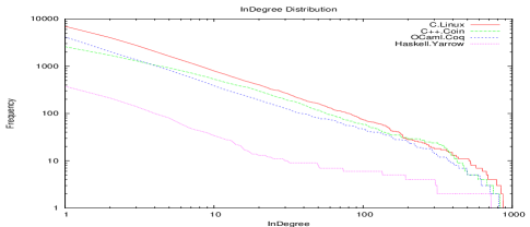
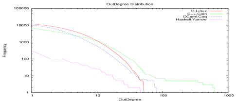
We use cumulative distribution to fit the data and we compute the likelihood measures for other distributions in order to improve the confidence using [8]. Figures 1 and 2 depict how four programs written in four different language paradigms compare; the indegree distribution permits power-law ($2.3\leq\gamma\simeq\leq 2.9$) while the outdegree distribution permits exponential distribution (Haskell results are coarse, but are valid). This observation, that in and out degree distributions differ consistently across languages, is expected as indegree and outdegree are conditioned very differently during the developmental process.

Outdegree has a strict budget; large, monolithic functions are difficult to read and reuse. Thus outdegree is minimized on a local, immediate scale. On the other hand, large indegree is implicitly encouraged, up to a point; indegree selection, however, happens in a non-local scale, over a much larger time period; usually backward compatibility permits lazy pruning/modifying of such nodes. Consequently one would expect the variability of outdegree – as depicted by the length of the errorbar, to be far less compared to that of the indegree. This is consistent with the observation (Fig. 3). Note that the tail of the outdegree is prominent in OCaml and C++: languages that allow highly stylized call composition.

Such observations are critical as distributions portend the accuracy of sample estimates. In particular, such distributions as power-law that permits non-finite mean and variance – consequently eluding central limit theorem, are very poor candidates for simple sampling based analyses; understanding the degree distribution is of both empirical and theoretical importance.

Figure 3: Average Degree

Consider the bug propagation process delineated in Section 3. Assuming that the inter-node bug propagation is Markovian, we could construct an irreducible, aperiodic, finite state space Markov chain (not unlike [6]) with bug introduction rate $\beta$ and debugging (immunization) rate $\delta$ as parameters. Note that this Markov chain has two absorbing states: all-infected or all-cured. Equipped with these notions, we could ask what is the minimal critical infection rate $\beta_{c}$ beyond which no amount of immunization will help to save the software; below $\beta_{c}$ the system exponentially converges to the good, all-cured absorbing state. It is known that for a sufficiently large power-law network with exponent in the range $2<\gamma\leq 3$, $\beta_{c}$ is zero [5]. Thus one is tempted to conclude that, provided Markovian assumption holds, it is statistically impossible to construct an all-reliable program. However that would be inaccurate as the sum of indegree and outdegree distribution indegree and outdegree need not follow power-law. However a recent study [25] establishes that, for finite networks, $\beta_{c}$ is bounded by the spectral diameter of the graph; in particular, $\beta_{c}=\frac{1}{\lambda_{1,A}}$, where $\lambda_{1,A}$ is the largest eigenvalue of the adjacency matrix. Figure 4 depicts the relation between $\lambda_{1,A}$ and the graph size, $n$. For a “robust” software, we require $\beta_{c}$ to be large, or equally, $\lambda_{1,A}$ to be small. However, it is evident from the plot that larger the graph, higher the $\lambda_{1,A}$. This trend is observed uniformly across languages. Thus, we are to conclude that large programs tend to be more fragile, confirming the established wisdom. Another equally important inference one can make from the indegree distribution is that uniform fault testing is bound to fail: should one is to build a statistically robust software, testing efforts ought to be heavily biased. These two inferences align closely with the common wisdom, except that these inferences are rigorously established (and party explained) using the statistical nature of call graphs.

Figure 4: Epidemic Threshold Vs $\mathbf{N}$

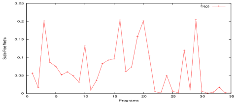
Scale Free Metric: Fig. 5 shows how scale-free metric for symmetrized call graphs vary with different programs. Two observations are critical: First, $S(g)$ is close to zero. This implies call graphs are scale-rich and not scale-free. This is of importance because in a truly scale-free networks, epidemics are even harder to handle; hubs are connected to hubs and the Markov chain rapidly converged to the all-infected absorption state. In scale-rich networks, as hubs tend to connect to lesser nodes, the rate of convergence is less rapid. Second, $S(g)$ appears to be language independent. Both near zero and higher $S(g)$s appear in all languages. Thus call graphs, though follow power-law for indegree, are not fractal like in the self-similarity sense.

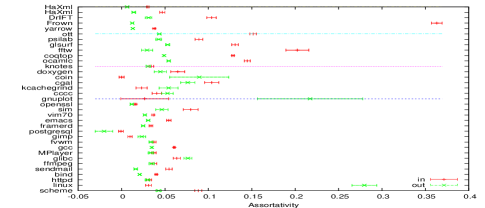
Degree Correlation: Fig 7 show how input-input (i-i) and output-output (o-o) degrees correlate with each other. These sets are weakly assortative, signifying hierarchical organization.

But finer picture evolves as far as languages are concerned. C programs appears to have very similar i-i and o-o profiles with o-o correlation being smaller and comparable to i-i correlation. In addition, C’s correlation measure is consistently less than that of other languages and is close to zero; thus, C programs exhibit as much i-i/o-o correlation as that of a random graph of similar size. In other words, if foo calls bar, the number of calls bar makes is independent of the number of calls foo made; this implies less hierarchical program structure as one would like the level $n$ functions to receive fewer calls compared to level $n-1$ functions. For instance, variance(list) is likely to receive fewer calls compared to sum(list); we would also like level $n$ functions to have higher outdegree compared to level $n-1$ functions. Thus, in a highly hierarchical design, i-i and o-o correlations would be mildly assortative, with i-i being more assortative. For C++, i-i and o-o differ and are not ordered consistently. OCaml and Haskell exhibit marked difference in correlations: as with C, the o-o correlation is close to zero; but, i-i correlation is orders of magnitude higher than o-o correlation. That is, OCaml forces nodes with “proportional” indegree to pair up. If foo is has an indegree X, bar is likely to receive, say, 2X indegree. One could interpret this result as a sign of stricter hierarchical organization in functional languages.

Figure 5: Scale Free Metric

Figure 6: Clustering Coefficient

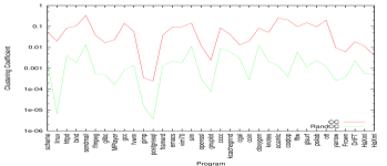
Clustering Coefficient: Fig. 6 depicts how the call graph clustering coefficients compare to clustering coefficients of random networks of same size. Computed clustering coefficients are orders of magnitude higher than their random counterpart signifying higher degree of clustering. Also, observe that $\ell$, as depicted is Fig. 8, is in the order of $\log n$. Together these observations make call graphs decidedly small world, irrespective of the source language.

We also have observed that average clustering coefficient for nodes of particular degree, $C(d_{i})$ follows power-law. That is, the plot of $d_{i}$ to $C(d_{i})$ follows the power-law with $C(d_{i})\propto d_{i}^{-1}$: high degree nodes exhibit lesser clustering and lower degree notes exhibit higher clustering. It is also observed that OCaml’s fit for this power-law is the one that had least misfit. Though we need further samples to confirm it, we believe functional languages exhibit cleaner, non-interacting hierarchy compared to both procedural and OO languages.

Figure 7: Assortativity Coefficient

Figure 8: Harmonic Geodesic Mean

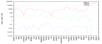
Component Statistics: Fig. 9 gives us the components statistics for the data set. It depicts the number of weakly connected components (#WCC), number of strongly connected components (#SCC), and fraction of nodes in the largest strongly connected component (%SCC).

#WCC is lower in C and OCaml. For C++ and Haskell, #WCC is higher compared to rest of the sample. This is an indication of lazy call resolution, coinciding with the delayed/lazy bindings encouraged by both the languages. The #SCC values are highest for OCaml. This observation, combined with reciprocity of OCaml programs, makes OCaml a language that encourages recursion at varying granularity. On the other end, C++ rates least against #SCC values.

Another important aspect in Fig. 9 is the observed values for %SCC; this fraction varies, surprisingly, from 1% to 30% of total number of nodes. C leads the way with some applications, notably vim and Emacs, measuring as much as 20 to 30% for %SCC. OCaml follows C with a moderate 2 to 6% while C++ measures 1% to 3%. We do not yet know why one third of an application cluster to form a SCC. Also, %SCC values say that certain languages, notably OCaml, and programs domains (Editors: Vim and Emacs) exhibit significant mutual connectivity.

Figure 9: Component Statistics

Figure 10: Betweenness - C.Linux

Edge Reciprocity: Fig. 11 shows the plot of edge reciprocity for various programs. Edge reciprocity is a measure of direct mutual recursion in the software. High reciprocity in a layered system implies layering inversion and we would, ideally, like a program to have negative reciprocity.

Most programs exhibit close to zero reciprocity: most call graphs exhibit as much reciprocity as that of random graphs of comparable size. None exhibit negative reciprocity, implying no statistically significant preferential selection to not to violate strict layering.

The software that had least reciprocity is the Linux kernel. Recursion of any kind is abhorred inside kernel as kernel-stack is a limited resource; besides, in a environment where multiple contexts/threads communicate using shared memory, mutual recursion could happen through continuation flow, not just as explicit control flow. Functional languages like OCaml naturally show higher reciprocity. Another curious observation is that compilers, both OCamlc and gcc, appear to have relatively higher reciprocity. This is the second instance where applications (Compilers: GCC and OCamlc) determining the graph property; this could be seen as a reflection of how compilers work: a great deal of the lexing, parsing and semantic algorithms that compilers are based on follow rich mutually recursive mathematical definitions.

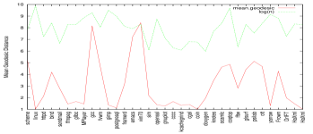
Clustering Profile: As we see in Fig 13, Clustering Profile indeed gives us a better insight. Y axis depicts the average clustering coefficient for nodes, say $i$ and $j$, that are connected by geodesic distance $d_{ij}$. In all the graphs observed, this average clustering increases up to $d_{ij}$=3 and falls rapidly as $d_{ij}$ increases further. We measured clustering profile for degrees one to ten and the clustering profile appears to be unimodal, reaching the maximum at $d_{ij}$=3, irrespective of language/program domain. It suggests that maximal clustering occurs between nodes that are separated exactly by five hops: clustering profile for a node $u$ is measured with $u$ removed; so $d_{ij}$=3 is 5 hops in the original graph. However exciting we find this result to be, we currently have no explanation for this phenomenon.

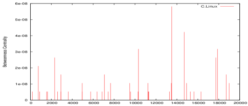
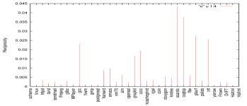
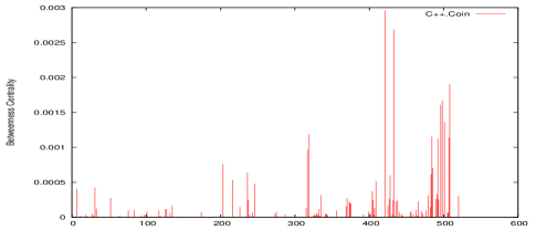
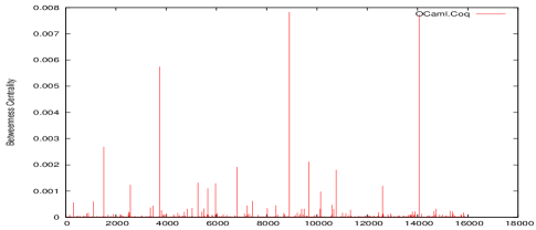
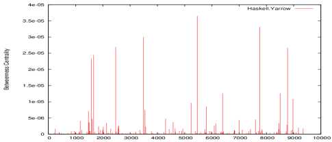
Betweenness: Fig. 10 to 15 depict how betweenness centrality is distributed – in different programs, written in different different languages. Note that betweenness is not distributed uniformly: it follows a rapidly decaying exponential distribution. This confirms our observation that importance of functions is distributed non-uniformly. Thus, by concentrating test efforts in functions that have higher betweenness – functions that are central to most paths – we could test the software better, possibly with less effort. An interesting line of investigation is to measure the correlation between various centrality measures and actual per function bug density in a real-world software.

Figure 11: Edge Reciprocity

Figure 12: Betweenness - C++.Coin

Figure 13: Clustering Profile for Neighbours reachable in $\mathbf{k}$+2 hops

7 Related Work

Understanding graph structures originating from various fields is an active field of research with vast literature; there is a renewed enthusiasm in studying graph structure of software and many studies, alongside ours, report that software graphs exhibit small-world and power-law properties.

[18] studies the call graphs and reports that both indegree and outdegree distributions follow power-law distributions and the graph exhibits hierarchical clustering. But [23] suggests that indegree alone follows power-law while the outdegree admits exponential distribution. [23] also suggests a growing network model with copying, as proposed in [15], would consistently explain the observations.

More recently, [4] studies the degree distributions of various meaningful relationships in a Java software. Many relationships admit power-law distributions in their indegree and exponential distribution in their out-degree. [22] studies the dynamic, points-to graph of objects in Java programs and found them to follow power-law.

Note that most work, excepting [4], do not rigorously compare the likelihood of other distributions to explain the same data. Power-law is notoriously difficult to fit and even if power-law is a genuine fit, it might not be the best fit [8].

Figure 14: Betweenness - OCaml.Coq

8 Conclusion & Future Work

We have studied the structural properties of large software systems written in different languages, serving different purposes. We measured various finer aspects of these large systems in sufficient detail and have argued why such measures could be useful; we also depicted situations where such measurements are practically beneficial. We believe our study is a step towards understanding software as an evolving graph system with distinct characteristics, a viewpoint we think is of importance in developing and maintaining large software systems.

There is lot that needs to be done. First, we need to measure the correlation between these precise quantities and the qualitative, rule of thumb understanding that developers usually possess. This helps us making such qualitative, albeit useful, observations rigorous. Second, we need to verify our finding over a much larger set to improve the inference confidence. Finally, graphs are extremely useful objects that are analysed in a variety of ways, each exposing relevant features; of these variants, the authors find two fields very promising: topological and algebraic graph theories. In particular, studying call graphs using a variant of Atkin’s A-Homotopy theory is likely to yield interesting results [3]. Also, spectral methods applied to call graphs is an area that we think is worth investigating.

Figure 15: Betweenness - Haskell.Yarrow

Appendix I

*	Lang	Name.Version	Appln. Domain	$\mathbf{N}$	$\mathbf{M}$
1	C	scheme.mit.7.7.1	Interpreter	2512	5610
2	C	linux.2.6.12.rc2	Kernel	20165	70010
3	C	httpd.2.2.4	Web Sever	1396	4014
4	C	bind.9.4.1	Name Server	4534	18874
5	C	sendmail.8.12.8	Mail Server	783	4064
6	C	ffmpeg.2007.05	Media Codecs	4207	11692
7	C	glibc.2.3.6	C Lib	4401	13972
8	C	MPlayer.1.0rc1	Media Player	7985	21744
9	C	gcc.4.0.0	C Compiler	10848	48847
10	C	fvwm.2.5.18	Win Manager	3312	12052
11	C	gimp.2.3.9	Image Editor	16021	88473
12	C	postgresql.8.2.3	R-DBMS	8517	41189
13	C	framerd.2.6.1	OO-DMBS	3490	17048
14	C	emacs.21.4	“Editor”	3872	13154
15	C	vim70	Editor	4489	18368
16	C	sim.outorder.3.0	$\mu$arch/ISA Sim	442	1089
17	C	openssl.0.9.8e	Crypto Lib	7078	21827
18	C	gnuplot.4.2.2	Graph Plotting	2191	7045
19	C++	cccc.3.1.4	Code Metrics	1654	5627
20	C++	kcachegrind.0.4	Cache Analyser	2593	8054
21	C++	cgal.3.3	CompGeom Lib	3151	7690
22	C++	coin.2.4.6	OpenGL 3D Lib	12963	51877
23	C++	doxygen.1.5.3	Doc Generator	11723	31889
24	C++	knotes.3.3	PIM	2174	4942
25	OCaml	ocamlc.opt.3.09	OCaml Compiler	4397	12732
26	OCaml	coqtop.opt.8	Theorem Prover	16126	51092
27	OCaml	fftw.3.2alpha2	FFT Computing	585	1011
28	OCaml	glsurf.2.0	OpenGL Surface	4003	9173
29	OCaml	psilab.2.0	Numeric Envirn	1888	4341
30	OCaml	ott.0.10.11	PL/Calculi Tool	4300	11193
31	Haskell	yarrow.1.2	Theorem Prover	9397	15199
32	Haskell	Frown.0.6.1	Parser Gen	6796	10218
33	Haskell	DrIFT.2.2.1	Typed Preproc	1428	3292
34	Haskell	HaXml.1.Validate	XML Validate	4117	7624
35	Haskell	HaXml.1.Xtract	XML grep	3909	5242

References

- [1] A. Abdo and A. de Moura. Clustering as a measure of the local topology of networks. In arXiv:physics/0605235, 2006.
- [2] S. Asur, S. Parthasarathy, and D. Ucar. An ensemble approach for clustering scalefree graphs. In LinkKDD workshop, 2006.
- [3] H. Barcelo, X. Kramer, R. Laubenbacher, and C. Weaver. Foundations of a connectivity theory for simplicial complexes. In Advances in Applied Mathematics, 2006.
- [4] G. Baxter and et al. Understanding the shape of java software. In OOPSLA, 2006.
- [5] M. Boguna, R. Pastor-Satorras, and A. Vespignani. Absence of epidemic threshold in scale-free networks with connectivity correlations. In arXiv:cond-mat/0208163, 2002.
- [6] S. Brin and L. Page. The anatomy of a large-scale hypertextual Web search engine. Computer Networks and ISDN Systems, 30(1–7):107–117, 1998.
- [7] J. A. Børretzen and R. Conradi. Results and experiences from an empirical study of fault reports in industrial projects. In PROFES, 2006.
- [8] A. Clauset and et al. Power-law distributions in empirical data. In arXiv.org:physics/0706.1062, 2007.
- [9] L. da F. Costa, F. A. Rodrigues, G. Travieso, and P. R. V. Boas. Characterization of complex networks: A survey of measurements. Advances In Physics, 56:167, 2007.
- [10] F. S. Diego Puppin. The social network of java classes. In ACM Symposium on Applied Computing, 2006.
- [11] P. Erdös and A. Rényi. On random graphs. In Publicationes Mathematicae 6, 1959.
- [12] D. Garlaschelli and M. I. Loffredo. Patterns of link reciprocity in directed networks. Physical Review Letters, 2004.
- [13] D. Hrimiuc. The rearrangement inequality - a tutorial: pims.math.ca/pi/issue2/page21-23.pdf, 2007.
- [14] http://projects.forked.de/graph tool/.
- [15] P. Krapivsky and S. Redner. Network growth by copying. Phys Rev E Stat Nonlin Soft Matter Phys, 2005.
- [16] L. Li, D. Alderson, R. Tanaka, J. Doyle, and W. Willinger. Towards a theory of scale-free graphs. In arXiv:cond-mat/0501169, 2005.
- [17] Y. Matsuo. Clustering using small world structure. In Knowledge-Based Intelligent Information and Engineering Systems, 2002.
- [18] C. R. Myers. Software systems as complex networks. In Physical Review, E68, 2003.
- [19] M. Newman. The structure and function of complex networks. In SIAM Review, 2003.
- [20] M. E. J. Newman. Assortative mixing in networks. Physical Review Letters, 89:208701, 2002.
- [21] D. E. Perry and W. M. Evangelist. An empirical study of software interface faults. In Symposium on New Directions in Computing, 1985.
- [22] A. Potanin, J. Noble, M. Frean, and R. Biddle. Scale-free geometry in oo programs. Comm. ACM, May 2005.
- [23] S. Valverde and R. V. Sole. Logarithmic growth dynamics in software networks. In arXiv:physics/0511064, Nov 2005.
- [24] S. Valverde and R. V. Sole. Hierarchical small worlds in software architecture. In arXiv:cond-mat/0307278, 2006.
- [25] Y. Wang, D. Chakrabarti, C. Wang, and C. Faloutsos. Epidemic spreading in real networks: An eigenvalue viewpoint. In Symposium on Reliable Distributed Computing, 2003.
- [26] A. Y. Wu, M. Garland, and J. Han. Mining scale-free networks using geodesic clustering. In ACM SIGKDD, 2004.
- [27] www.csn.ul.ie/ mel/projects/codeviz/.