COSMOGRAIL: the COSmological MOnitoring of
GRAvItational Lenses

Gravitationally lensed quasars can be used to map the mass distribution in lensing galaxies and to estimate the Hubble constant H₀ by measuring the time delays between the quasar images. Here we report the measurement of two independent time delays in the quadruply imaged quasar WFI J2033–4723  ($z=1.66$). Our data consist of $R$-band images obtained with the Swiss 1.2 m EULER telescope located at La Silla and with the 1.3 m SMARTS telescope located at Cerro Tololo. The light curves have 218 independent epochs spanning 3 full years of monitoring between March 2004 and May 2007, with a mean temporal sampling of one observation every 4th day. We measure the time delays using three different techniques, and we obtain $\Delta t_{B-A}=35.5\pm 1.4$ days (3.8%) and $\Delta t_{B-C}=62.6\leavevmode\nobreak\ ^{+\,4.1}_{-\,2.3}\leavevmode\nobreak\ \ \hbox{days}\leavevmode\nobreak\ \ (^{+\,6.5\%}_{-\,3.7\%})$, where $A$ is a composite of the close, merging image pair. After correcting for the time delays, we find $R$-band flux ratios of $F_{A}/F_{B}=2.88\pm 0.04$, $F_{A}/F_{C}=3.38\pm 0.06$, and $F_{A1}/F_{A2}=1.37\pm 0.05$ with no evidence for microlensing variability over a time scale of three years. However, these flux ratios do not agree with those measured in the quasar emission lines, suggesting that longer term microlensing is present. Our estimate of H₀ agrees with the concordance value: non-parametric modeling of the lensing galaxy predicts H₀  = 67 ${}^{+13}_{-10}$ km s^-1 Mpc^-1, while the Single Isothermal Sphere model yields H₀ = 63 ${}^{+7}_{-3}$ km s^-1 Mpc^-1(68% confidence level). More complex lens models using a composite de Vaucouleurs plus NFW galaxy mass profile show twisting of the mass isocontours in the lensing galaxy, as do the non-parametric models. As all models also require a significant external shear, this suggests that the lens is a member of the group of galaxies seen in field of view of WFI J2033–4723.

Figure 1: The 6.3′ $\times$ 6.3′ field of view around WFI J2033–4723. This image is the central part of a combination of 418 $R$-band frames obtained with the 1.2m EULER Telescope with a total exposure time of 48 hours and a mean seeing of 1.3″. The three stars PSF1–3 used to model the Point Spread Function (PSF) and the 7 reference stars S4–10 used for frame alignment and flux calibration are indicated.

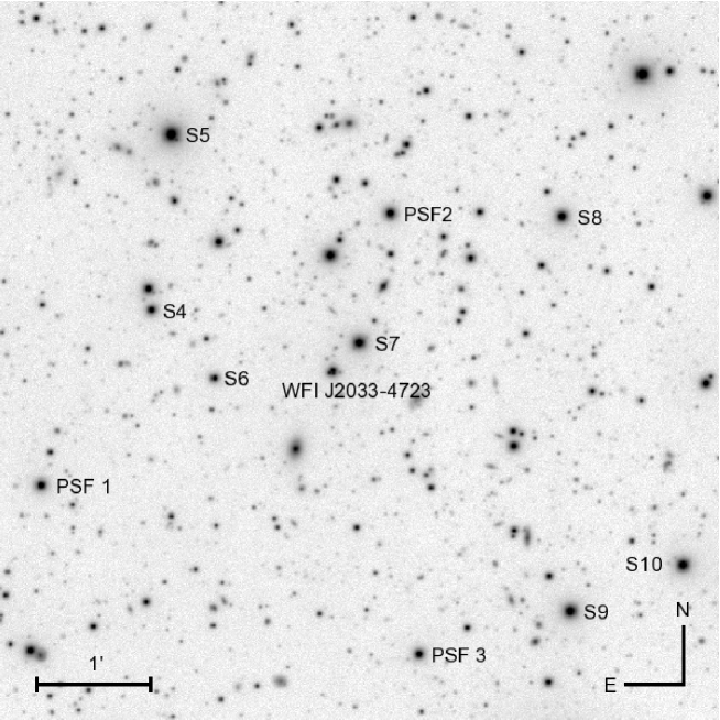
1 Introduction

When a quasar is gravitationally lensed and we observe multiple images of the source there are light travel time differences between the images. Any intrinsic variation of the quasar is observed at different times in each image with a measurable “time delay” between them. Refsdal (1964) first showed that time delays provide a means of determining the Hubble constant H₀ independent of any local distance calibrator, provided a mass model can be inferred for the lensing galaxy. Conversely, one can also assume H₀ in order to study the distribution of the total mass in the lensing galaxy.

During the past 25 years, time delays have been measured in only 17 systems, at various accuracy levels (see Oguri 2007, for a review). As the error in the time delay propagates directly into H₀, it is important to make it as small as possible. Unfortunately, most existing time delays have uncertainties of the order of 10% that are comparable to the current uncertainties in H₀. This uncertainty can be reduced by increasing the sample of lenses with known time delays, and by simultaneously fitting all lenses in the sample with a common value for H₀ (Saha et al. 2006b, a; Coles 2008).

COSMOGRAIL is an optical monitoring campaign that aims to measure time delays for a large number of gravitationally lensed quasars to accuracies of a few percent using a network of 1- and 2-m class telescopes. The first result of this campaign was the measurement of the time delay in the doubly imaged quasar SDSS J1650+4251 to an accuracy of 3.8% based on two observing seasons of data (Vuissoz et al. 2007). COSMOGRAIL complements a second monitoring group whose most recent results are a delay for HE 1104-1805 (Poindexter et al. 2007). In this paper we present time-delay measurements for the quadruply imaged quasar WFI J2033–4723 based on merging 3 years of optical monitoring data from the two groups. In a companion effort, Morgan et al. (2008) analyzed the merged data for the two-image lens QJ0158–4325, succeeding in measuring the size of the source accretion disk but failing to measure a time delay due to the high amplitude of the microlensing variability in this system.

WFI J2033–4723  (20^h33^m42$\aas@@fstack{s}$08, –47°23′43$\aas@@fstack{\prime\prime}$0; J2000.0) was discovered by Morgan et al. (2004) and consists of 4 images of a $z=1.66$ quasar with a maximum separation of 2.5″. The lens galaxy was identified by Morgan et al. (2004) and has a spectroscopic redshift of $z_{\rm lens}$ = $0.661\pm 0.001$ (Eigenbrod et al. 2006). The lens appears to be the member of a group, with at least 6 galaxies within 20″ of the lens (Morgan et al. 2004), and we will have to account for this environment in any lens model.

We describe the monitoring data and its analysis in Sect. 2 In Sect. 3 we present the near-IR Hubble Space Telescope (HST) observations that we used to obtain accurate differential astrometry of the lens components and surface photometry of the lens galaxy. We estimate the time delays in Sect. 4 and model them using parametric (Sect. 5) and non-parametric (Sect. 6) models for the mass distribution of the lens galaxy. We summarize our results in Sec. 7.

2 Photometric monitoring

Our 3-year photometric monitoring of WFI J2033–4723 was carried out from March 2004 to May 2007 with the 1.2 m EULER telescope and the 1.3 m SMARTS telescope located in Chile at La Silla and the Cerro Tololo Interamerican Observatory (CTIO), respectively. WFI J2033–4723  was monitored from both sites for three years during its visibility window from early March to mid-December.

The 1.2m EULER telescope is equipped with a 2048$\times$2048 CCD camera which has 0.344″ pixels and produces an image with an 11′ field of view. The mean sampling of the EULER data is one epoch every five days, where each epoch consists of five dithered 360s images taken with an R-band filter. The worst gaps due to weather or technical problems are 2–3 weeks. The EULER data set consists of 141 epochs of data obtained between May 2004 and May 2007. The image quality varies between 0.9″ and 2.0″  FWHM over 3 years, with a median of 1.4″.

The 1.3m SMARTS telescope is equipped with the dual-beam ANDICAM (DePoy et al. 2003) camera. Here we use only the optical channel which has 0.369″  pixels and a 6.5′$\times$6.3′ field of view. The mean sampling of the SMARTS data is one epoch every eight days, with three 300s exposures at each epoch. The SMARTS data set consists of 77 epochs of data obtained between March 2004 and December 2006. The seeing on the images varies between 0.5″  and 2.0″, with a median of 1.4″.

The combined data set consists of 218 observing epochs comprising 956 images covering the common field of view shown in Fig. 1. The average temporal sampling when WFI J2033–4723  was visible is one observation every 4 days over a period of three years, one of the best sets of monitoring data available for a lensed quasar.

Figure 2: Result of the simultaneous deconvolution of the 956 $R$-band images (EULER+SMARTS) of WFI J2033–4723. The pixel size of this image is half the pixel size of the EULER detector, i.e., 0.172″, and the resolution is 2 pixels Full-Width-Half-Maximum, i.e., 0.344″. The field of view is 22″ on a side. Two galaxies $G2$ and $G3$ are seen to the West and North of the main lensing galaxy $G1$. $G3$ is part of a group included in the lens modeling, while $G1$ and $G2$ are modeled individually (see Sect. 5).

The EULER data are reduced using the automated pipeline described in Vuissoz et al. (2007) and the SMARTS data with the SMARTS pipeline, using standard methods. The reduced frames are then aligned and interpolated to a common reference frame, one of the best-seeing (1″) EULER images, taken on the night of 5 April 2006. The 10 stars (PSF1–3 and S4–10) shown in Fig. 1 are used to determine the geometric transformation needed for each EULER and SMARTS image to match the reference frame. The transformation includes image parity, rotation, shifting and rescaling. These 10 stars are also used to determine the photometric zero point of each image relative to the reference image. After interpolation, cosmic rays are removed using the L.A.Cosmic algorithm (van Dokkum 2001). We check that no data pixels are mistakenly removed by this process.

The light curves of the quasars are measured by simultaneously deconvolving all the images using the MCS algorithm (Magain et al. 1998). This method has already been successfully applied to the monitoring data of several lensed quasars (e.g. Vuissoz et al. 2007; Hjorth et al. 2002; Burud et al. 2002a, b). The deconvolved images have a pixel scale of 0.172″ (one-half the pixel scale of the EULER data) and are constructed to have a Gaussian PSF with a 2 pixel (0.344″) FWHM. The Point Spread Function (PSF) for each of the 956 images is constructed from the three stars PSF1–3 (see Fig. 1). During the deconvolution process, the relative positions of the quasar images are held fixed to the values derived from fitting the HST images in Sect. 3, while their fluxes are allowed to vary from frame to frame. The flux, position and shape of the lensing galaxy are the same for all frames, but the values vary freely as part of the fit.

Figure 3: Our $R$-band light curves obtained for WFI J2033–4723  as well as for the reference star S6 (see Fig. 1). The magnitudes are given in relative units. The filled symbols correspond to the EULER observations while the SMARTS data points are marked by open symbols. Components $A_{1}$ and $A_{2}$ were summed into one single component $A$. The curves have been shifted in magnitude for visibility, as indicated in the figure.

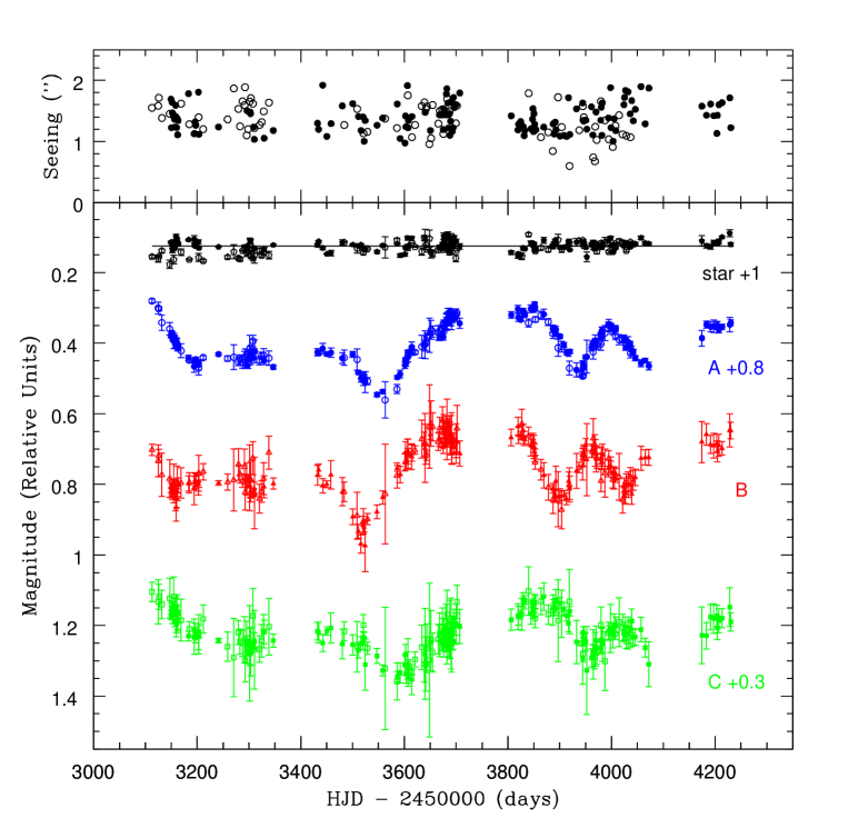
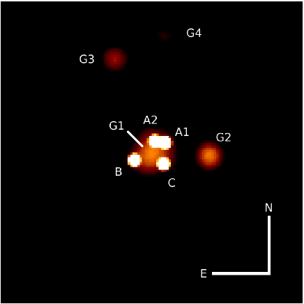
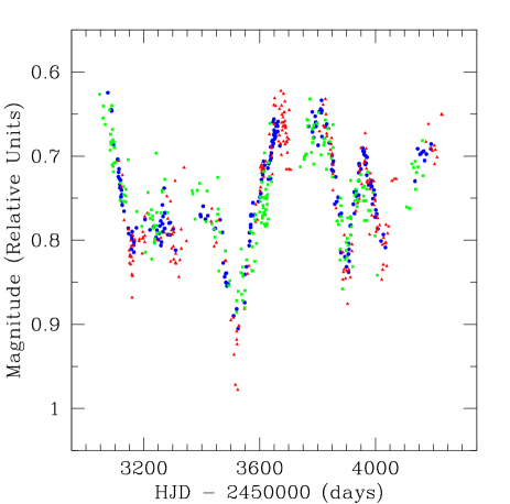
Fig. 2 shows an example of a deconvolved image. It is clear that we will have no difficulty estimating the fluxes of components $B$ and $C$ separately. Components $A_{1}$ and $A_{2}$, however, are separated by only 0.724″, which is only twice the resolution of our deconvolved images, and remain partially blended after deconvolution. Since the delay between these images should be very small, we will sum the fluxes of the two images and consider only the light curve of the total flux $A=A_{1}+A_{2}$. The resulting $R$-band light curves are displayed in Fig. 3.

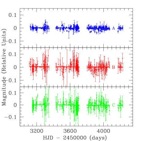
We also display in Fig. 3 the deconvolved light curve of the isolated star $S6$, which has roughly the same color as WFI J2033–4723. Each point is the mean of the images taken at a given epoch and the error bar is the 1$\sigma$ standard error of the mean. The light curve is flat, with a standard deviation over the 3 years of monitoring of $\sigma_{\rm{tot}}=0.010$ mag about its average, which is roughly consistent with the mean error bar of $\sigma_{\rm{mean}}=0.006$ mag of the individual epochs.

The dispersion of the points in the star’s light curve reflects both statistical errors and systematic errors from the photometric calibrations and the construction of the PSF. To the extent that all the light curves suffer from the same systematic errors, we can correct the quasar’s light curves by subtracting the residuals of the star’s light curve from each of them. We then define the uncertainty in a quasar’s light curve as the quadrature sum of the uncertainties in the two light curves. This procedure will increase the photon noise but should minimize the systematic errors.

3 HST Near-IR Imaging

Figure 4: Left: Deep NICMOS2 image, taken in the F160W-band. This image is a combination of 4 frames, for a total exposure time of 46 minutes. North is up and East to the left. The field of view is 4″  on a side. Middle: Simultaneous deconvolution of the individual NICMOS images (see text), using the MCS deconvolution algorithm. The PSF in this image is an analytical Gaussian with 2 pixels Full-Width-at-Half-Maximum (FWHM), i.e., the resolution is 0.075″. The pixel size is 0.035″, i.e., oversampled by a factor of two compared to the original pixel size. Right: Residual map of the deconvolution, with the cut levels set to $\pm 5\sigma$. Only minor structures are seen in the center of the sharpest objects, which is acceptable given the quality of the NICMOS PSF.

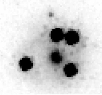
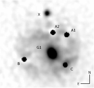
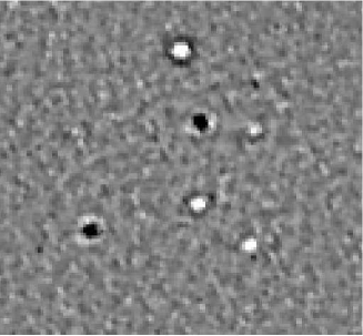
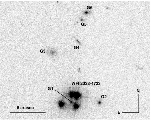
We determine the relative positions of the lens components and the light profile for the main lens galaxy $G1$ and its closest neighbor $G2$ (see Fig. 2) by analyzing our HST images of the system. These data were obtained in the framework of the CASTLES program (Cfa-Arizona Space Telescope LEns Survey), which provides HST images for all known gravitationally lensed quasars. We deconvolve these images using a modified version of the MCS deconvolution algorithm for images with poor knowledge of the PSF (Magain et al. 2007). We previously used this approach to unveil the faint Einstein ring and the lensing galaxy hidden in the glare of the quasar images of the so-called “cloverleaf” HE1413+117 (Chantry & Magain 2007). We analyze the Near Infrared Camera and Multi-Object Spectrometer (NICMOS) F160W (H-band) images obtained with the NIC2 camera. The data consist of four dithered MULTIACCUM images with a total exposure time of 2752 s and a mean pixel scale of 0.07568″(Krist & Hook 2004). We calibrate the images using CALNICA, the HST image reduction pipeline, subtract constants for each quadrant of NIC2 to give each image a mean background of zero, and create a noise map for each frame.

The images are simultaneously deconvolved in a manner similar to that used for the EULER and SMARTS data. The NICMOS frames lack any PSF stars, so we construct the PSF using the quasar images themselves in the iterative method of Chantry & Magain (2007). We first estimate the PSF of each frame using Tiny Tim (Krist & Hook 2004) and then we deconvolve them to have the final Gaussian PSF. During the deconvolution, each image is decomposed into a set of point sources and any extended flux. The latter is then reconvolved to the resolution of the original data and subtracted from the four initial frames, leading to images with far less contamination by extended structures. Four new PSFs are estimated from these new images, and we carry out a new deconvolution. The process is repeated until the residual maps are close to being consistent with the estimated noise (e.g. Courbin et al. 1998). In this case, convergence is reached after three iterations and the final reduced $\chi^{2}$ is 3.59. The final deconvolved image shown in Fig. 4 has half the pixel scale of the initial images and a Gaussian PSF with a FWHM of 0.075″.

As part of the MCS deconvolution we also fit analytical models to the main lens galaxy ($G1$) and its nearby companion $G2$. The main lens is an early-type galaxy (Eigenbrod et al. 2006), as its companion is likely to be, so we use elliptical de Vaucouleurs profiles for both. The uncertainties are estimated by the scatter of the measurements from a separate set of fits to each independent image. We also estimate that there are systematic errors in the astrometry from the NICMOS pixel scale and focal plane distortions of order 2 milli-arcseconds based on our earlier fits to the NICMOS data of H1413+117 (Chantry & Magain 2007). These systematic errors are compatible with the Lehár et al. (2000) comparison of NICMOS and VLBI astrometry for radio lenses.

The relative astrometry and photometry of the lens components and of the lensing galaxies $G1$ and $G2$ are given in Table 1. Coordinates are relative to image $B$, in the same orientation as Fig 4. The photometry is in the Vega system. For each measurement, we give the $1\sigma$ internal error bars, to which a systematic error of 2 milli-arcsec should be added. The models for $G1$ and $G2$ are presented in Table 2, with the effective semi-major and semi-minor axes of the light distribution $a_{0}$ and $b_{0}$. Each measurement is accompanied by its $1\sigma$ error bar.

Table 1: Relative astrometry and photometry for the four components of WFI J2033–4723  and for the lensing galaxies $G1$ and $G2$.

ID	$\Delta\alpha$ (″)	$\Delta\delta$ (″)	Magnitude
B	0.	0.	17.77 $\pm$ 0.02
A1	$-2.1946$ $\pm$ 0.0004	1.2601 $\pm$ 0.0003	17.16 $\pm$ 0.02
A2	$-1.4809$ $\pm$ 0.0004	1.3756 $\pm$ 0.0005	17.52 $\pm$ 0.02
C	$-2.1128$ $\pm$ 0.0003	$-0.2778$ $\pm$ 0.0003	17.88 $\pm$ 0.02
G1	$-1.4388$ $\pm$ 0.0019	0.3113 $\pm$ 0.0008	18.59 $\pm$ 0.03
G2	$-5.4100$ $\pm$ 0.0006	0.2850 $\pm$ 0.0003	18.14 $\pm$ 0.02

Table 2: Shape parameters for the main and secondary lensing galaxies.

Obj.	PA (∘)	Ellipticity	$a_{0}$ (″)	$b_{0}$ (″)
G1	27.8 $\pm$ 4.3	0.18 $\pm$ 0.03	0.665 $\pm$ 0.036	0.556 $\pm$ 0.025
G2	6.4 $\pm$ 3.1	0.15 $\pm$ 0.02	0.389 $\pm$ 0.004	0.334 $\pm$ 0.005

4 Time delay measurement

We measure the time delays between the blended light curve of $A_{1}$/$A_{2}$ and images $B$ and $C$ using three different techniques: $i$ the minimum dispersion method of Pelt et al. (1996); $ii$ the polynomial method of Kochanek et al. (2006); and $iii$ the method of Burud et al. (2001). Since WFI J2033–4723  shows well-defined variations (see Fig. 3), it is already clear by visual inspection that $\Delta t_{B-A}\sim 35$ days and $\Delta t_{B-C}\sim 65$ days.

4.1 Minimum dispersion method

Figure 5: Example of a dispersion curve as obtained from the minimum dispersion method, for components $B$ and $A$. The position of the parabola minimum gives the time delay. Each point is separated by 2 days, i.e. about half the data mean sampling. The time delay indicated here is for only one realization of the boot-strap procedure (see text).

Figure 6: Variation of the dispersion function minimum $D_{\rm{min}}$ (red solid curves), as a function of the magnitude shift used for the normalization (see Sect. 4.1). Each $D_{\rm{min}}$ corresponds to a different estimate of the time delay, indicated on the blue dotted curves. The final time delay is the one with the lowest $D_{\rm{min}}$. The top panel is for the $B$-$A$ time delay, the bottom one for $B$-$C$. Time delays indicated here are for only one realization of the boot-strap procedure (see text).

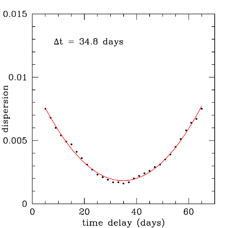
In the minimum dispersion method, time delays are computed for pairs of light curves using a cross-correlation technique that takes into account irregular sampling. The two light curves are first normalized to have zero mean. Then, one of the light curves is used as a reference and the second curve is shifted relative to it by a range of time delays. For each delay, we calculate the mean dispersion between the shifted points and their nearest temporal neighbors in the reference light curve. The best time-delay estimate is the one that minimizes this dispersion function. Since the mean sampling of our curves is one epoch every four days and since there is a limit to the number of time delays that can be tested independently, we test time delays in steps of 2 days. Fig. 5 shows an example of a dispersion curve where we have then fit a parabola and set the best time delay to be the one corresponding to the minimum of the parabola.

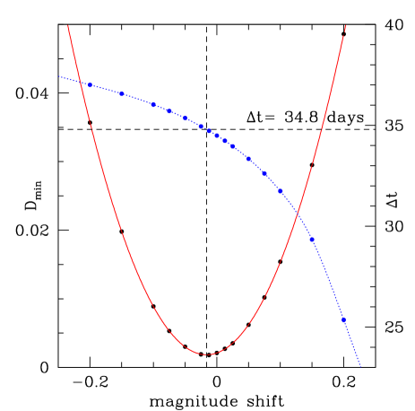
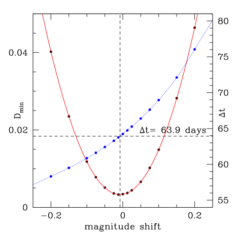
There is, however, a complication in the step of normalizing the light curves, arising from sampling the light curve of each lensed image over a different time period of the intrinsic source variability (Vuissoz et al. 2007). We solve this problem by computing the dispersions as a function of a small magnitude shift $\Delta m$ in the normalization, measuring both the minimum dispersion $D_{min}(\Delta m)$ and the best fitting time delay $\Delta t(\Delta m)$ as shown in Fig. 6. Our final value for the delay is the one corresponding to the shift $\Delta m$ that minimizes the overall dispersion.

We then estimate the uncertainties by randomly perturbing the data points, based on a Gaussian distribution with the width of the measurement errors, and computing the dispersions and time delays again. We define the uncertainties by the $1\sigma$ dispersion in the results for 100,000 trials (Vuissoz et al. 2007). The resulting uncertainty estimates are symmetric about the mean, so our final estimates based on this method are

$$\Delta t_{B-A}= 35.6\pm 1.3\leavevmode\nobreak\ \ \hbox{days}\leavevmode\nobreak\ \ (3.6\%)$$

$$\Delta t_{B-C}= 64.6\pm 3.4\leavevmode\nobreak\ \ \hbox{days}\leavevmode\nobreak\ \ (5.3\%)$$ (1)

While we have not taken microlensing effects into account for this analysis, it should matter little, as the method is not very sensitive (Eigenbrod et al. 2005) to the very low amplitude microlensing variability observed for this system (see Sect. 4.2).

4.2 Polynomial fit of the light curves

Figure 7: Top: Best polynomial fit to the light curves, which are shifted vertically for display purpose. Bottom: The residuals of the fit.

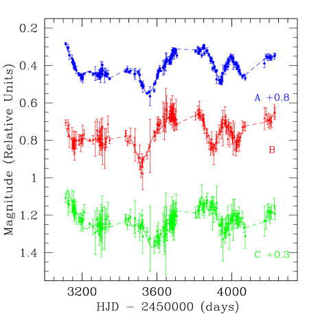
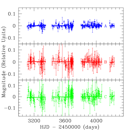
In the polynomial method (Kochanek et al. 2006), the intrinsic light curve of the source is modeled as a polynomial that is simultaneously fit to all three light curves. Each quasar image has an additional low order polynomial to model slow, uncorrelated variability due to microlensing. We increase the source polynomial order for each season until the improvement in the $\chi^{2}$ statistics of the fits cease to be significant. This results in using polynomial orders of 11, 10, 17 and 4 for the four seasons of data. The low amplitude microlensing variations are modeled with a simple linear function for the four seasons. Fig. 7 shows the best fits to the data and the residuals from the model. The effects of microlensing in this system are very small, with variations of only $\sim 0.01$ mag over three years. As with the minimum dispersion method, we estimate the uncertainties by randomly perturbing the light curves 100,000 times and using the standard deviation of the trials as the error estimates to find that

$$\Delta t_{B-A}= 35.0\pm 1.1\leavevmode\nobreak\ \ \hbox{days}\leavevmode\nobreak\ \ (3.0\%)$$

$$\Delta t_{B-C}= 61.2\pm 1.5\leavevmode\nobreak\ \ \hbox{days}\leavevmode\nobreak\ \ (2.4\%)$$ (2)

4.3 Numerical modeling of the light curves

Figure 8: Top: The light curves of the quasar images shown along with the best numerical model. Bottom: The residuals of the fit.

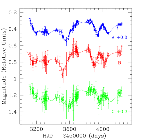
Our last approach is based on the method described in Burud et al. (2001), which determines the time delay between a pair of light curves using a gridded numerical model for the source light curve. For a series of time delays, we fit the data with a flux ratio between the two curves, and a linear trend for microlensing on each full light curve. The numerical source model is smoothed on the scale of the temporal sampling, based on a smoothing function weighted by a Lagrange multiplier. The best time delay is the one that minimizes the $\chi^{2}$ between the model and data points.

This method has several advantages: first, none of the data light curves is taken as a reference: they are all treated on an equal basis. Furthermore, as the model is purely numerical, no assumption is made on the shape of the quasar’s intrinsic light curve (except that it is sufficiently smooth). Finally, a model light curve is obtained for the intrinsic variations of the quasar, as for the polynomial fit method (see Sect. 4.2).

We have applied this method to the two pairs of light curves of WFI J2033–4723. The resulting fits to the light curves and their residuals are shown in Fig. 8. Using a Monte Carlo method to estimate the uncertainties, we find from 7,000 trials (adding normally distributed random errors with the appropriate standard deviation on each data point) :

$$\Delta t_{B-A}= 36.0\pm 1.5\leavevmode\nobreak\ \ \hbox{days}\leavevmode\nobreak\ \ (4.2\%)$$

$$\Delta t_{B-C}= 61.9\leavevmode\nobreak\ ^{+\,6.7}_{-\,0.5}\leavevmode\nobreak\ \ \hbox{days}\leavevmode\nobreak\ \ (^{+\,11\%}_{-\,1\%})$$ (3)

We note a secondary peak in the $\Delta t_{B-C}$ Monte Carlo distribution, around 69 days, in addition to the main peak at 61.9 days. There is, however, no evidence of such a secondary peak in the results of the minimum dispersion method and the polynomial fitting technique. This translates into an asymmetrical error bar on the result obtained with the numerical fitting of the light curves, and is taken into account in our final estimate of the time delay between quasar images $B$ and $C$.

4.4 Final time delays

Figure 9: Light curves of the three quasar images, shifted by their respective time delay and flux ratio. The blue circles correspond to image $A$, the red triangles to $B$ and the green squares to $C$.

For the final delay estimate we adopt the unweighted mean of the three methods, and we take as uncertainties the quadrature sum of the average statistical error and the dispersion of the results from the individual methods about their mean. Our final estimate of the time delays is

$$\Delta t_{B-A}= 35.5\pm 1.4\leavevmode\nobreak\ \ \hbox{days}\leavevmode\nobreak\ \ (3.8\%)$$

$$\Delta t_{B-C}= 62.6\leavevmode\nobreak\ ^{+\,4.1}_{-\,2.3}\leavevmode\nobreak\ \ \hbox{days}\leavevmode\nobreak\ \ (^{+\,6.5\%}_{-\,3.7\%})$$ (4)

We cannot measure the time delay between the individual $A_{1}$ and $A_{2}$ light curves, but values larger than $\Delta t_{A1-A2}=2$ days are incompatible with any of the models we consider in the following section. We can nevertheless estimate the flux ratio between $A_{1}$ and $A_{2}$. After correcting for the time delays, we find that the $R$-band flux ratios between the images are

$$\frac{F_{A}}{F_{B}}=2.88\pm 0.04,\leavevmode\nobreak\ \ \frac{F_{A}}{F_{C}}=3.38\pm 0.06,\leavevmode\nobreak\ \ \frac{F_{A1}}{F_{A2}}=1.37\pm 0.05$$ (5)

Fig. 9 displays the light curves obtained for the three quasar images, after shifting by the time delays and flux ratios. Note that these flux ratios differ from those measured by Morgan et al. (2004) from the MgII broad emission lines, probably due to long-term microlensing (on a longer scale than our monitoring 3-year baseline), as discussed in the next section.

Figure 10: Environment of WFI J2033–4723 as seen in an HST/ACS F814 (I-band) image. The main lens galaxy $G1$ and the close companion $G2$ were included in our analysis of the NICMOS image, and here we have labeled additional group members as $G3$-$G6$.

Table 3: Result of the parametric lens modeling.

Name	Comp.	mass	e, $\theta_{e}$	$\gamma$, $\theta_{\gamma}$	#d.o.f.	$\chi^{2}$	$h$	Comments
SIE+$\gamma$		b=0.96	0.21, (20.8)	0.187, 7.4	1	15.3	-	Time delays not used
SIE+$\gamma$		b=0.94	0.13, (30.5)	0.063, 24.6	2	3.6	$0.79^{+0.04}_{-0.02}$	$G_{\rm group}$ included
SIE+$\gamma$		b=0.97	0.16, 84.4	0.059, 46.9	1	0.30	$0.63^{+0.07}_{-0.03}$	$G_{\rm group}$ included
dVC+$\gamma$		b=2.71	0.20, (20.1)	0.305, 9.7	1	34.4	-	Time delays not used
dVC+$\gamma$		b=2.83	0.18, 83.1	0.116, 64.5	1	0.01	$0.92^{+0.06}_{-0.03}$	$G_{\rm group}$ included
NFW+$\gamma$		$\kappa_{s}$=0.20	0.16, (27.4)	0.070, -3.6	1	0.38	-	$r_{s}$=10″(fixed); time delays not used
NFW+$\gamma$		$\kappa_{s}$=0.21	0.15, 85.7	0.079, 9.5	1	0.06	$0.29^{+0.03}_{-0.03}$	$r_{s}$=10″(fixed); $G_{\rm group}$ included
NFW+$\gamma$		$\kappa_{s}$=0.09	0.15, 85.4	0.076, 30.6	1	0.01	$0.63^{+0.10}_{-0.08}$	$r_{s}$=1″(fixed); $G_{\rm group}$ included
dVC+NFW+$\gamma$	Light	b=1.56	(0.17), (29.3)	0.057, 37.0	-	-	-	$R_{e}=0.608$″(fixed)
	Halo	$\kappa_{s}$=0.082	0.065, (29.3)		1	6.33	$0.78^{+0.12}_{-0.10}$	$r_{s}$=10″(fixed); $G_{\rm group}$ included
dVC+NFW+$\gamma$	Light	b=1.53	(0.16), (26.4)	0.075, 27.5	-	-	-	same model as above, with
	Halo	$\kappa_{s}$=0.10	0.43, 89.8		3	3.2	0.69${}^{+0.20}_{-0.10}$	flux ratios included

5 Parametric modeling

5.1 Observational constraints

We constrain the mass models of WFI J2033–4723 using the positions of the four lensed images, the position of the lens galaxy $G1$ and the two delay measurements, for a total of 12 constrains. Except when indicated, we do not use the image flux ratios because they can be affected by extinction (Falco et al. 1999; Jean & Surdej 1998) and milli-lensing by substructures (Mao & Schneider 1998). We can also constrain the structure of $G1$ given its ellipticity $e$, position angle $\theta_{e}$ and effective radius $R_{e}$ to the extent that these properties are correlated with those of its dark matter halo. Although a possible mismatch between the light and mass distributions is not impossible, we adopt the formal errors of 0.002″  on the position of the lens $G1$ (Table 2). This is motivated by the small offset between the centers of mass and light found by Yoo et al. (2006) in a sample of four lensing galaxies.

Finally, WFI J2033–4723 is located in a group of galaxies, labeled $G2$-$G6$ in Fig. 10. We include $G2$ as a singular isothermal sphere (SIS) in all our models since it is close (4″) and of similar luminosity to $G1$. As Morgan et al. (2004), we are unable to successfully model the system without including $G2$. When enough observational constraints are available we further add galaxies $G3$-$G6$ as a SIS mass distribution located at the barycenter $G_{\rm group}$ of the group. In all models we include an external shear of amplitude $\gamma$ and position angle $\theta_{\gamma}$ that represents the gravitational perturbations due to mass unaccounted for explicitly. We also experiment with including mass at the position of object $X$ (Fig. 4, 2″  North of $G1$) and find that doing so does not improve the models.

We consider a sequence of standard mass models for $G1$, including a singular isothermal ellipsoid (SIE), a de Vaucouleurs (dVC) model and a NFW model (Navarro et al. 1997), and we fit the data using LENSMODEL (v1.99g) (Keeton 2001). The results are summarized in Table 3, where columns $\#1$ and $\#2$ describe the model family, and $\#3$ the mass parameter (either the Einstein radius $b$ in arcseconds or the mean mass surface density $\kappa_{s}$, as defined in Keeton 2001). Column $\#4$ is for the ellipticity $e$ and PA $\theta_{e}$ of the lens $G1$. Note that the measured PA of $G1$ is $\theta=27.8^{\circ}$ (Table 2). Column $\#5$ gives the external shear amplitude $\gamma$ and PA $\theta_{\gamma}$, $\#6$ the number of degrees of freedom for each model, and $\#7$ the resulting reduced $\chi^{2}$. Column $\#8$ finally shows the best estimate for $h=$H₀$/100$. A minus sign in this column means that time delays are not used as constraints. All angles are given positive East of North, and values given in parentheses are fitted to the observations. All models assume $\Delta t_{A1-A2}=2$ days and include the companion galaxy $G2$, with a resulting mass $0.1\,m_{G1}<m_{G2}<m_{G1}$.

5.2 SIE Models

Our first model consists of an SIE for $G1$, an SIS for $G2$ and an external shear. When we fit only the image positions but include a prior on the position angle $\theta_{e}$ (from Table 1) we do not find a good fit unless the constraint on the position of the lensing galaxy is relaxed. The prior on the position angle is justified by statistical studies finding correlations between the position angles but not the axis ratios of the visible and total mass distributions (Ferreras et al. 2008; Keeton et al. 1997). With the inclusion of the time delays we have enough constraints to add the group halo to the model. With the position angle of $G1$ constrained, we obtain poor fits to the data with reduced $\chi^{2}=3.6$ for $N_{\rm dof}=2$. When we leave the position angle free, we find good fits but the model PA is $55^{\circ}$ from the observed. These models have Hubble parameters of $h\simeq 0.63^{+0.07}_{-0.03}$ with the spread dominated by the degeneracies between the ellipticity and the shear.

5.3 De Vaucouleurs Models

Next we consider a constant mass-to-light ratio model of the lens galaxy based on a De Vaucouleurs model. The position angle and the effective radius $R_{e}=0.608$″  (the geometric mean of the semi-axes in Table 1, corresponding to 4 kpc for $h=0.72$) are constrained by the values measured for the galaxy. This model does not fit well the lens configuration ($\chi^{2}\sim 34.4$), mainly due to the small uncertainty on the lens galaxy position. When we include the time delays we find a good fit ($\chi^{2}\simeq 0.01$) as long as we allow $G1$ to be misaligned with respect to the observed galaxy. As expected from the reduced surface density compared to the SIE model (Kochanek 2002), we find a much higher value for the Hubble parameter, $h=0.92$.

5.4 NFW Models

We use an NFW model with a fixed break radius of $r_{s}=10$″ (40 kpc), where the break radius is related to the virial radius through the concentration $c=R_{\rm vir}/r_{s}$. Since $r_{s}$ lies well outside the Einstein radius of the lens, its particular value is not important. This model is not realistic by itself because the shallow $\rho\propto 1/r$ central density cusp of the model will lead to a visible central image. We again find that we can fit the astrometry well even when the position angle of the lens is constrained, but we cannot do so after including the time delays unless we allow the model of $G1$ to be misaligned relative to the light. In any case, this model leads to a fifth image about 3 mag fainter than $A$ that should be visible on our NICMOS data. This NFW model has a higher surface density near the Einstein ring than the SIE model, so we find a lower value for the Hubble parameter of $h\simeq 0.29$. Using an unphysically small break radius of $r_{s}=1$″ raises the density and hence the Hubble parameter to $h\simeq 0.63$.

5.5 De Vaucouleurs plus NFW Models

As our final, and most realistic, parametrized model we combine a dVC model constrained by the visible galaxy with an NFW model for the halo. The two components are first constrained to have the same position and position angle, the parameters of the dVC model are constrained by the observations, and the NFW model has a fixed $r_{s}=10$″ break radius. This model leads to a poor fit, with $\chi^{2}=6.33$ for $N_{\rm dof}=1$. When we free the PA of the NFW model, we find an acceptable fit for $N_{\rm dof}=0$, but the misalignment of the NFW model relative to the optical is $40^{\circ}$.

We can further constrain the model by including the three MgII emission line flux ratios from Morgan et al. (2004). We use the line flux ratios instead of those obtained from the light curves, because they should be insensitive to microlensing. With these three additional constraints we still find that the $89.8^{\circ}$ position angle of the NFW model is strongly misaligned from the $26.4^{\circ}$ position angle of the dVc model, indicating a twisting of the mass isocontours. The model has a reduced $\chi^{2}$ of $3.2$ for $N_{\rm dof}=3$. The model flux ratios are significantly different from the constraints. We find $F_{A}/F_{B}=2.81$, $F_{A}/F_{C}=5.01$, and $F_{A1}F_{A2}=1.26$ while Morgan et al. (2004) report $F_{A}/F_{B}=2.55\pm 0.60$, $F_{A}/F_{C}=2.02\pm 0.35$, and $F_{A1}/F_{A2}=1.61\pm 0.35$. The match of the flux ratios is better if we do not include the constraints from the time delays. In all cases, $F_{B}/F_{C}$ is the most “anomalous” flux ratio, as also found by Morgan et al. (2004). While the differences between the line and continuum flux ratios suggests the presence of long-term microlensing, we see no evidence for the time variability in the flux ratios expected from microlensing. We also note that the broad line flux ratios vary with wavelength (Morgan et al. 2004), which suggests that dust extinction may as well be affecting the flux ratios.

Figure 11: Distribution of H₀ from 1000 non-parametric models. The bottom-axis gives the Hubble time, the top-axis H₀ in km s^-1 Mpc^-1.

6 Non-parametric modeling

We use the non-parametric PixeLens (Saha & Williams 2004) method as our second probe of the mass distribution. This approach has the advantage that it makes fewer assumptions about the shape of the $G1$ than the ellipsoidal parametric models. The models include priors on the steepness of the radial mass profile, imposes smoothness criteria on the profile and we restrict to models symmetric about the lens center. We include two point masses to represent $G2$ and the group. We run 1000 trial models at a resolution of $\sim 0.23\arcsec$/pixel which are constrained to fit the image positions and the time delays exactly. For each model we vary the Einstein radii of $G2$ and the group over the ranges 0.03″  $<R_{E}(G2)<$ 3″and 0.3″ $<R_{E}({\rm group})<$ 5″, respectively. Apart from the inclusion of these additional point masses, the method and priors are as explained in detail in Coles (2008). A test, where the technique is used to infer H₀ from a N-body and hydro simulated lens, and an additional discussion of the priors are described in Read et al. (2007). Fig. 11 shows the resulting probability distribution for H₀ from the 1000 models. The median value of the distribution is

$$\hbox{H${}_{\rm 0}$}=67.1\leavevmode\nobreak\ ^{+13.0}_{-9.9}\leavevmode\nobreak\ \ \hbox{km s${}^{-1}$ Mpc${}^{-1}$}$$ (6)

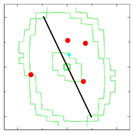
where the error bars are at 68% confidence. As already illustrated by our parametric modeling, the predicted H₀  value depends on the density gradient of the models. Fig. 12 shows the mean surface density contours of the models, and we see a twisting of the contours away from that of the visible galaxy in the outer regions.

Figure 12: Mean mass distribution from 1000 pixellated lens models. The red dots are the quasar images and the blue dot the source position. The thick solid line indicates the observed major axis of the lensing galaxy. Each tick-mark measures 1″. The third contour from the outside traces the critical mass density $\Sigma_{\rm crit}=1.19\,10^{11}$ M_⊙ arcsec^-2, and the others are drawn logarithmically from the critical one (each contour is 2.5 larger/smaller than the previous one). North is to the top and East to the left.

7 Conclusions

By combining data from COSMOGRAIL and the SMARTS 1.3m telescope we measure two independent time delays in the quadruply imaged quasar WFI J2033–4723 (Morgan et al. 2004). The fractional uncertainties of $\sim 4\%$ are among the best obtained so far from an optical monitoring. We obtain the light curves of the quasar images using the MCS deconvolution photometry algorithm (Magain et al. 1998) and then measure time delays using three different approaches with a final estimate of

$$\Delta t_{B-A}= 35.5\pm 1.4\leavevmode\nobreak\ \ \hbox{days}\leavevmode\nobreak\ \ (3.8\%)$$

$$\Delta t_{B-C}= 62.6\leavevmode\nobreak\ ^{+\,4.1}_{-\,2.3}\leavevmode\nobreak\ \ \hbox{days}\leavevmode\nobreak\ \ (^{+\,6.5\%}_{-\,3.7\%})$$ (7)

where $A$ is the mean light curve of the blended of quasar images $A_{1}$ and $A_{2}$. We find little evidence of microlensing in this system, which makes WFI J2033–4723  a very good system for measuring clean time delays.

The parametric models are consistent with concordance value of H₀ when the lens galaxy has an isothermal mass profile out to the radius of the Einstein ring. As expected, the models allow higher (lower) values as the mass distribution is more centrally concentrated (extended) using de Vaucouleurs (NFW) mass distribution. The non-parametric models predict H₀ = 67.1 ${}^{+13.0}_{-9.9}$ km s^-1 Mpc^-1.

The addition of the time delays as a constraint on the lens models does not alter the mismatch between the observed and predicted image flux ratios. The largest flux ratio anomaly is the 45% difference between the MgII flux ratios found for images B/C. Morgan et al. (2004) also noted that the $F_{B}$/$F_{C}$ flux ratio varies with wavelength, suggesting the presence of chromatic microlensing. The lack of significant variability in the flux ratio over our three year monitoring period suggests either that the effective source velocities in this lens are very low or that the affected images lie in one of the broad demagnified valleys typical of microlensing magnification patterns for low stellar surface densities.

Several galaxies close to the line of sight have a significant impact on the mass modeling. We generally model the potential as the sum of a main lensing galaxy $G1$, a companion galaxy $G2$ ($\sim$ 4″ West of $G1$), and a nearby group ($\sim$ 9″ North of $G1$). Both the parametric and non-parametric models suggest that the isodensity contours of $G1$ itself must be twisted, with some evidence that the outer regions are aligned with the tidal field of the group rather than the luminous galaxy. This could indicate that $G1$ is a satellite rather than the central galaxy of the group (e.g. Kuhlen et al. 2007). The twisting seems to be required even though the angular structure of the potential can be adjusted through the companion galaxy $G2$, an external tidal shear, and in some cases a group halo. Clarifying this issue requires more constraints such as detailed imaging of the Einstein ring image of the quasar host, measuring the redshifts of the nearby galaxies, and measuring the velocity dispersion of $G1$.

Table 4: Photometry of WFI J2033–4723, as in Fig. 3. The Julian date corresponds to HJD-2450000 days.

HJD	seeing [”]	mag $A$	$\sigma_{A}$	mag $B$	$\sigma_{B}$	mag $C$	$\sigma_{C}$	telescope
3112.86	1.55	1.330	0.006	1.752	0.016	2.155	0.027	SMARTS
3124.85	1.58	1.350	0.017	1.783	0.045	2.183	0.063	SMARTS
3125.84	1.71	1.352	0.006	1.769	0.019	2.169	0.036	SMARTS
3131.83	1.38	1.392	0.022	1.823	0.061	2.190	0.041	SMARTS
3146.90	1.45	1.409	0.018	1.834	0.053	2.173	0.056	SMARTS
3149.34	1.69	1.430	0.005	1.859	0.015	2.221	0.013	EULER
3150.32	1.22	1.425	0.009	1.874	0.014	2.202	0.016	EULER
3151.35	1.64	1.421	0.006	1.866	0.016	2.211	0.017	EULER
3152.29	1.47	1.432	0.009	1.864	0.029	2.214	0.031	EULER
3154.30	1.42	1.439	0.006	1.876	0.011	2.210	0.014	EULER
3154.84	1.42	1.443	0.022	1.847	0.055	2.168	0.056	SMARTS
3156.27	1.36	1.434	0.007	1.853	0.017	2.238	0.016	EULER
3157.39	1.23	1.444	0.012	1.867	0.026	2.196	0.026	EULER
3158.36	1.59	1.454	0.008	1.887	0.037	2.208	0.037	EULER
3159.29	1.40	1.453	0.012	1.915	0.040	2.240	0.043	EULER
3160.32	1.23	1.446	0.009	1.889	0.026	2.246	0.024	EULER
3161.37	1.37	1.451	0.015	1.841	0.043	2.211	0.049	EULER
3162.33	1.11	1.464	0.009	1.871	0.024	2.236	0.029	EULER
3163.22	1.34	1.460	0.008	1.853	0.021	2.217	0.025	EULER
3168.93	1.62	1.471	0.020	1.846	0.043	2.235	0.060	SMARTS
3183.37	1.78	1.491	0.007	1.848	0.022	2.280	0.014	EULER
3184.78	1.28	1.498	0.006	1.845	0.029	2.260	0.021	SMARTS
3194.30	1.12	1.516	0.016	1.863	0.046	2.282	0.050	EULER
3195.28	1.12	1.501	0.006	1.845	0.018	2.264	0.020	EULER
3196.36	1.32	1.504	0.008	1.837	0.018	2.273	0.017	EULER
3197.18	1.26	1.495	0.006	1.843	0.015	2.281	0.018	EULER
3202.41	1.81	1.511	0.015	1.849	0.031	2.282	0.037	EULER
3202.76	1.40	1.520	0.020	1.818	0.051	2.275	0.056	SMARTS
3203.41	1.12	1.508	0.009	1.841	0.017	2.267	0.017	EULER
3211.74	1.20	1.491	0.006	1.814	0.023	2.231	0.040	SMARTS
3241.31	1.24	1.481	0.004	1.846	0.007	2.293	0.007	EULER
3258.72	1.36	1.493	0.008	1.844	0.023	2.310	0.042	SMARTS
3270.73	1.87	1.490	0.035	1.838	0.088	2.341	0.111	SMARTS
3279.64	1.53	1.502	0.011	1.794	0.045	2.270	0.034	SMARTS
3282.63	1.25	1.494	0.011	1.821	0.025	2.296	0.035	SMARTS
3287.60	1.66	1.505	0.016	1.840	0.019	2.300	0.037	SMARTS
3291.56	1.60	1.497	0.025	1.800	0.050	2.290	0.066	SMARTS
3292.57	1.89	1.489	0.023	1.872	0.050	2.349	0.061	SMARTS
3295.62	1.10	1.483	0.016	1.835	0.045	2.297	0.060	SMARTS
3296.15	1.50	1.512	0.008	1.857	0.022	2.302	0.023	EULER
3298.57	1.20	1.508	0.014	1.840	0.016	2.312	0.023	SMARTS
3301.62	1.65	1.464	0.036	1.831	0.094	2.329	0.136	SMARTS
3302.09	1.48	1.486	0.011	1.854	0.033	2.309	0.051	EULER
3303.06	1.45	1.496	0.015	1.870	0.030	2.330	0.035	EULER
3303.58	1.71	1.477	0.018	1.837	0.052	2.324	0.069	SMARTS
3307.59	1.62	1.444	0.016	1.776	0.047	2.223	0.078	SMARTS
3309.08	1.24	1.492	0.002	1.873	0.012	2.309	0.010	EULER
3310.13	1.03	1.473	0.007	1.863	0.019	2.293	0.022	EULER
3310.55	1.22	1.473	0.033	1.874	0.101	2.319	0.112	SMARTS
3320.55	1.27	1.499	0.013	1.891	0.041	2.317	0.037	SMARTS
3324.56	1.32	1.485	0.010	1.870	0.030	2.294	0.046	SMARTS
3328.52	1.49	1.485	0.019	1.834	0.045	2.267	0.047	SMARTS
3329.07	1.05	1.499	0.011	1.857	0.031	2.269	0.033	EULER
3338.51	1.64	1.492	0.021	1.760	0.047	2.254	0.080	SMARTS
3347.06	1.18	1.518	0.006	1.847	0.016	2.293	0.019	EULER
3432.39	1.30	1.475	0.010	1.824	0.028	2.266	0.025	EULER
3434.40	1.20	1.477	0.006	1.809	0.017	2.270	0.029	EULER
3442.37	1.92	1.465	0.015	1.854	0.020	2.300	0.024	EULER
3450.39	1.08	1.481	0.005	1.850	0.010	2.265	0.012	EULER
3458.40	1.29	1.477	0.013	1.823	0.040	2.257	0.043	EULER
3480.38	1.58	1.493	0.015	1.871	0.040	2.302	0.042	EULER
3483.86	1.27	1.491	0.022	1.871	0.028	2.266	0.027	SMARTS
3500.40	1.62	1.482	0.008	1.942	0.022	2.305	0.029	EULER
3508.85	1.53	1.496	0.030	1.939	0.066	2.311	0.072	SMARTS
3511.34	1.41	1.533	0.005	1.983	0.020	2.320	0.022	EULER
3516.36	1.18	1.549	0.011	2.019	0.026	2.301	0.019	EULER
3520.41	1.40	1.545	0.012	1.965	0.025	2.293	0.025	EULER
3520.87	1.13	1.556	0.014	1.955	0.036	2.249	0.030	SMARTS
3522.41	1.00	1.545	0.006	1.970	0.014	2.287	0.018	EULER
3524.38	1.34	1.560	0.029	2.024	0.074	2.361	0.073	EULER
3528.83	1.16	1.558	0.010	1.948	0.016	2.314	0.018	SMARTS
3547.35	1.26	1.596	0.006	1.928	0.019	2.336	0.021	EULER
3558.23	1.38	1.587	0.005	1.887	0.019	2.377	0.015	EULER
3562.86	1.37	1.611	0.051	1.877	0.142	2.371	0.173	SMARTS
3585.76	1.22	1.580	0.013	1.825	0.035	2.409	0.052	SMARTS
3586.27	1.61	1.546	0.005	1.804	0.008	2.395	0.015	EULER
3592.04	1.05	1.537	0.011	1.822	0.024	2.384	0.029	EULER
3601.19	0.97	1.512	0.009	1.788	0.024	2.362	0.029	EULER
3602.21	1.42	1.497	0.006	1.760	0.030	2.333	0.030	EULER
3603.27	1.24	1.507	0.008	1.784	0.024	2.387	0.027	EULER
3606.21	1.91	1.490	0.013	1.757	0.035	2.363	0.039	EULER
3606.72	1.75	1.487	0.016	1.763	0.041	2.355	0.068	SMARTS
3607.18	1.22	1.477	0.008	1.766	0.018	2.395	0.020	EULER
3608.17	1.34	1.475	0.006	1.760	0.012	2.366	0.019	EULER
3614.32	1.41	1.461	0.015	1.771	0.036	2.403	0.043	EULER
3614.70	1.07	1.476	0.003	1.761	0.023	2.383	0.009	SMARTS
3620.69	1.27	1.475	0.004	1.753	0.012	2.346	0.021	SMARTS
3633.64	1.58	1.460	0.032	1.721	0.054	2.311	0.063	SMARTS
3638.66	1.64	1.454	0.013	1.736	0.034	2.359	0.052	SMARTS
3640.24	1.47	1.454	0.039	1.747	0.098	2.331	0.129	EULER
3641.58	1.53	1.450	0.022	1.737	0.057	2.359	0.077	SMARTS
3643.61	1.57	1.434	0.011	1.768	0.014	2.315	0.069	SMARTS
3648.60	0.96	1.428	0.048	1.686	0.118	2.348	0.218	SMARTS
3650.11	1.18	1.421	0.006	1.709	0.015	2.298	0.016	EULER
3651.55	1.05	1.412	0.027	1.678	0.064	2.293	0.085	SMARTS
3654.58	1.60	1.417	0.015	1.687	0.040	2.326	0.055	SMARTS
3665.55	1.29	1.420	0.020	1.729	0.025	2.289	0.042	SMARTS
3668.06	1.43	1.433	0.010	1.722	0.020	2.271	0.023	EULER
3668.52	1.50	1.415	0.014	1.690	0.031	2.276	0.062	SMARTS
3672.10	1.43	1.432	0.007	1.732	0.014	2.302	0.018	EULER
3673.52	1.53	1.411	0.014	1.669	0.039	2.253	0.053	SMARTS
3675.05	1.19	1.432	0.009	1.745	0.017	2.296	0.026	EULER
3675.52	1.12	1.395	0.011	1.686	0.034	2.271	0.042	SMARTS
3676.07	1.53	1.406	0.014	1.707	0.038	2.293	0.046	EULER
3677.11	1.50	1.408	0.011	1.697	0.024	2.281	0.033	EULER
3678.07	1.46	1.402	0.012	1.716	0.026	2.283	0.027	EULER
3680.07	1.43	1.394	0.007	1.712	0.023	2.290	0.034	EULER
3680.51	1.49	1.388	0.021	1.701	0.043	2.240	0.051	SMARTS
3681.10	1.78	1.395	0.018	1.706	0.037	2.289	0.032	EULER
3682.12	1.86	1.387	0.023	1.729	0.052	2.303	0.056	EULER
3682.51	1.70	1.389	0.023	1.673	0.064	2.218	0.069	SMARTS
3684.07	1.63	1.365	0.013	1.694	0.031	2.273	0.042	EULER
3685.10	1.22	1.391	0.010	1.710	0.028	2.292	0.032	EULER
3686.07	1.44	1.380	0.008	1.695	0.024	2.305	0.032	EULER
3687.07	1.45	1.362	0.011	1.682	0.026	2.286	0.029	EULER
3687.51	1.50	1.375	0.009	1.705	0.031	2.262	0.083	SMARTS
3688.10	1.10	1.386	0.012	1.733	0.030	2.270	0.029	EULER
3689.06	1.33	1.379	0.018	1.713	0.031	2.305	0.037	EULER
3690.08	1.65	1.380	0.021	1.711	0.056	2.273	0.100	EULER
3691.05	1.65	1.383	0.029	1.719	0.072	2.302	0.079	EULER
3692.03	1.64	1.382	0.011	1.762	0.031	2.279	0.041	EULER
3693.06	1.17	1.378	0.007	1.729	0.020	2.268	0.021	EULER
3694.06	1.22	1.378	0.004	1.730	0.014	2.256	0.012	EULER
3695.06	1.72	1.370	0.008	1.724	0.021	2.297	0.021	EULER
3696.07	1.55	1.367	0.013	1.742	0.020	2.230	0.026	EULER
3699.52	1.30	1.370	0.017	1.727	0.048	2.246	0.057	SMARTS
3700.07	1.60	1.376	0.012	1.762	0.028	2.246	0.032	EULER
3701.53	1.58	1.365	0.006	1.692	0.066	2.183	0.047	SMARTS
3707.07	1.79	1.394	0.015	1.763	0.035	2.253	0.048	EULER
3806.39	1.42	1.370	0.010	1.717	0.023	2.234	0.030	EULER
3819.38	1.19	1.353	0.010	1.686	0.026	2.225	0.037	EULER
3820.34	1.28	1.377	0.011	1.710	0.024	2.222	0.027	EULER
3824.39	1.32	1.384	0.004	1.712	0.012	2.219	0.013	EULER
3826.89	1.25	1.371	0.017	1.679	0.042	2.218	0.046	SMARTS
3829.37	1.24	1.358	0.007	1.697	0.017	2.177	0.020	EULER
3831.39	1.09	1.366	0.006	1.720	0.020	2.185	0.019	EULER
3832.41	1.18	1.370	0.005	1.723	0.011	2.178	0.013	EULER
3839.87	1.79	1.393	0.011	1.714	0.026	2.153	0.069	SMARTS
3844.41	1.21	1.353	0.011	1.739	0.030	2.216	0.031	EULER
3847.40	1.37	1.352	0.005	1.732	0.010	2.188	0.011	EULER
3848.39	1.54	1.350	0.009	1.725	0.020	2.204	0.025	EULER
3849.39	1.16	1.351	0.005	1.746	0.015	2.199	0.017	EULER
3850.37	1.46	1.354	0.008	1.744	0.032	2.200	0.027	EULER
3851.34	1.28	1.339	0.007	1.757	0.020	2.187	0.025	EULER
3852.35	1.18	1.352	0.006	1.767	0.018	2.184	0.018	EULER
3852.87	1.19	1.383	0.007	1.787	0.019	2.230	0.027	SMARTS
3863.79	1.07	1.371	0.011	1.809	0.029	2.181	0.038	SMARTS
3869.36	1.23	1.368	0.015	1.824	0.036	2.168	0.039	EULER
3877.88	1.15	1.390	0.010	1.858	0.037	2.219	0.028	SMARTS
3886.86	0.84	1.422	0.015	1.893	0.040	2.207	0.043	SMARTS
3887.42	1.29	1.406	0.006	1.861	0.014	2.199	0.023	EULER
3889.40	1.12	1.415	0.005	1.884	0.017	2.204	0.017	EULER
3891.42	1.32	1.424	0.005	1.881	0.017	2.199	0.014	EULER
3892.40	1.19	1.412	0.009	1.841	0.043	2.177	0.029	EULER
3896.88	1.72	1.463	0.024	1.892	0.078	2.236	0.116	SMARTS
3900.39	1.09	1.430	0.006	1.883	0.020	2.187	0.016	EULER
3903.79	1.23	1.460	0.015	1.922	0.053	2.217	0.067	SMARTS
3908.33	1.10	1.455	0.008	1.882	0.015	2.202	0.018	EULER
3913.28	1.08	1.476	0.007	1.891	0.017	2.222	0.015	EULER
3917.12	1.72	1.477	0.010	1.841	0.026	2.244	0.023	EULER
3918.84	0.60	1.521	0.020	1.851	0.048	2.182	0.091	SMARTS
3919.33	1.11	1.474	0.006	1.860	0.034	2.209	0.013	EULER
3932.40	1.53	1.526	0.020	1.812	0.049	2.297	0.061	EULER
3937.73	1.18	1.537	0.008	1.802	0.015	2.301	0.006	SMARTS
3944.22	1.63	1.522	0.022	1.797	0.040	2.343	0.073	EULER
3944.78	1.58	1.544	0.005	1.765	0.017	2.330	0.022	SMARTS
3945.35	1.35	1.510	0.007	1.764	0.015	2.269	0.016	EULER
3946.32	1.33	1.517	0.007	1.758	0.015	2.291	0.017	EULER
3946.63	1.39	1.531	0.010	1.768	0.030	2.278	0.025	SMARTS
3950.27	1.35	1.489	0.006	1.737	0.017	2.296	0.025	EULER
3952.24	1.20	1.488	0.047	1.780	0.102	2.377	0.125	EULER
3961.31	1.57	1.463	0.009	1.755	0.019	2.342	0.026	EULER
3964.09	1.11	1.449	0.004	1.752	0.011	2.322	0.018	EULER
3964.75	0.74	1.474	0.021	1.719	0.055	2.331	0.070	SMARTS
3967.78	0.67	1.450	0.011	1.738	0.029	2.340	0.033	SMARTS
3968.76	1.24	1.448	0.020	1.761	0.038	2.317	0.048	SMARTS
3970.22	1.48	1.447	0.011	1.778	0.037	2.293	0.041	EULER
3971.75	1.02	1.453	0.013	1.776	0.029	2.325	0.036	SMARTS
3979.17	1.35	1.426	0.003	1.778	0.013	2.313	0.017	EULER
3979.75	1.66	1.452	0.018	1.840	0.031	2.248	0.050	SMARTS
3980.27	1.56	1.435	0.018	1.774	0.031	2.291	0.035	EULER
3981.25	1.10	1.415	0.010	1.786	0.024	2.293	0.036	EULER
3982.25	1.63	1.417	0.013	1.767	0.031	2.303	0.048	EULER
3987.55	1.34	1.421	0.021	1.818	0.068	2.351	0.083	SMARTS
3994.14	1.38	1.396	0.007	1.805	0.024	2.265	0.025	EULER
3994.64	1.03	1.400	0.017	1.776	0.022	2.272	0.021	SMARTS
3998.12	1.88	1.404	0.010	1.798	0.025	2.258	0.068	EULER
3999.11	1.22	1.401	0.008	1.800	0.015	2.263	0.013	EULER
4002.57	0.91	1.416	0.010	1.837	0.024	2.279	0.035	SMARTS
4003.10	1.00	1.405	0.005	1.817	0.015	2.271	0.013	EULER
4005.10	1.37	1.414	0.011	1.831	0.032	2.248	0.031	EULER
4007.62	1.26	1.429	0.011	1.834	0.011	2.273	0.017	SMARTS
4008.17	1.18	1.407	0.007	1.820	0.016	2.248	0.022	EULER
4014.53	1.43	1.440	0.014	1.829	0.067	2.241	0.069	SMARTS
4021.58	1.12	1.439	0.011	1.894	0.038	2.256	0.038	SMARTS
4024.15	1.60	1.435	0.009	1.852	0.020	2.272	0.023	EULER
4025.10	1.72	1.442	0.007	1.882	0.022	2.266	0.025	EULER
4027.09	1.84	1.463	0.008	1.876	0.030	2.254	0.029	EULER
4028.57	1.09	1.456	0.006	1.844	0.024	2.295	0.019	SMARTS
4032.06	1.81	1.446	0.015	1.850	0.037	2.271	0.046	EULER
4036.07	1.45	1.452	0.007	1.849	0.022	2.258	0.022	EULER
4036.53	1.07	1.478	0.014	1.828	0.026	2.295	0.016	SMARTS
4039.05	1.67	1.470	0.012	1.877	0.030	2.237	0.034	EULER
4042.04	1.34	1.475	0.008	1.839	0.027	2.283	0.025	EULER
4046.04	1.52	1.492	0.007	1.830	0.023	2.283	0.023	EULER
4057.05	1.90	1.507	0.010	1.776	0.034	2.261	0.034	EULER
4065.06	1.29	1.499	0.006	1.774	0.022	2.313	0.027	EULER
4072.06	1.87	1.514	0.011	1.774	0.023	2.359	0.064	EULER
4174.40	1.58	1.436	0.022	1.730	0.058	2.277	0.080	EULER
4183.40	1.43	1.397	0.010	1.709	0.031	2.279	0.037	EULER
4191.40	1.61	1.404	0.015	1.737	0.026	2.226	0.036	EULER
4197.36	1.42	1.402	0.017	1.740	0.035	2.230	0.042	EULER
4203.39	1.13	1.400	0.011	1.734	0.025	2.223	0.031	EULER
4204.39	1.43	1.400	0.011	1.756	0.030	2.256	0.034	EULER
4207.37	1.60	1.411	0.009	1.739	0.031	2.236	0.034	EULER
4213.41	1.63	1.404	0.007	1.748	0.019	2.229	0.027	EULER
4228.34	1.71	1.397	0.020	1.697	0.047	2.198	0.055	EULER
4230.31	1.22	1.392	0.008	1.697	0.024	2.240	0.025	EULER

Table 4: continued.