Disentanglement of two harmonic oscillators in relativistic motion

Abstract

We study the dynamics of quantum entanglement between two Unruh-DeWitt detectors, one stationary (Alice), and another uniformly accelerating (Rob), with no direct interaction but coupled to a common quantum field in (3+1)D Minkowski space. We find that for all cases studied the initial entanglement between the detectors disappears in a finite time (“sudden death”). After the moment of total disentanglement the correlations between the two detectors remain nonzero until late times. The relation between the disentanglement time and Rob’s proper acceleration is observer dependent. The larger the acceleration is, the longer the disentanglement time in Alice’s coordinate, but the shorter in Rob’s coordinate.

I Introduction

A causally disconnected (spacelike separated) pair of qubits or atoms on the same time slice can be quantum correlated and entangled. This evokes the notion of “nonlocality” as an innate feature of quantum entanglement, the precise meaning of which is a topic of sustained interest and some controversy. When one examines the quantum entanglement across the event horizon of a black hole, the notion of “nonlocality” acquires an additional layer of meaning, pertaining not only to quantum correlations in ordinary (Minkowski) spacetime but also to some nontrivial (global) spacetime structure.

When the atoms are coupled with quantum fields, the situation becomes more interesting. Interaction with the quantum fields will induce decoherence of the atoms and affect the entanglement between them. It is known that the behavior of quantum entanglement is in general very different from decoherence. For the dynamics of quantum entanglement between two qubits different environmental settings could lead to very different results. (Compare, e.g, YE04 ; FicTan06 ; ASH06 ). Here we add in another dimension of consideration, that arising from nontrivial global structure of spacetime such as the existence of an event horizon, as in the spacetime of a black hole (Schwarzschild) or a uniformly accelerated detector (UAD). Specifically, how quantum entanglement between two detectors across the event horizon, one stationary and another uniformly accelerating, would evolve in time and how causality effects including that of retarded mutual influences would play out in these processes. This is an important ingredient for the establishment of relativistic quantum information theory.

Alsing and Milburn AM03 considered the quantum entanglement between two detectors (a quantum object with internal degrees of freedom), one is inertial (Alice) and the other is in relativistic motion (Bob, but when in uniform acceleration, they call it Rob) . Using the fidelity of the teleportation as a measure of entanglement, they claimed that the entanglement is degraded in noninertial frames due to the Unruh effect Unr76 . In their treatment, both detectors are made of cavities, and the qubits are constructed by using “single particle excitations of the Minkowski vacuum states in each of the cavities” of a scalar field. However, as is pointed out by Schützhold and Unruh SU05 , the introduction of cavities alters the boundary conditions in the derivations of the Unruh effect Unr76 ; DeW79 ; BD , and the evolution of the field modes depends on the way the cavity is accelerated. Furthermore, if Rob’s cavity is stationary in its local frame, then there is no particle creation inside, otherwise one has to take into account the dynamical Casimir effect SU05 .

Without the trouble associated with the cavity, Fuentes-Schuller and Mann FSM05 consider free field modes in Minkowski space and assume the inertial Alice and the accelerated Rob are observers sensitive to different single modes. Suppose the quantum field is in a maximally entangled state of these two modes and the uniformly accelerated Rob is always in the right Rindler wedge, then from the negativity of the observed reduced density matrix (which is obtained by integrating out the mode in the left Rindler wedge originally sensitive to Rob at rest but undetectable when Rob is accelerated), Fuentes-Schuller and Mann claimed that the field state is always entangled if Rob’s acceleration is finite, and because of the Unruh effect, the larger Rob’s acceleration, the smaller the entanglement between the two modes. Note that the entanglement here is not between qubits or anything localized in Alice or Rob’s hands; It is the entanglement between the two modes spread in the whole Minkowski space and observed locally by Alice and Rob without considering the back-reaction of the field on the detector. Note also that both the fidelity in AM03 and the negativity in FSM05 are independent of time. Thus there is no dynamics in these two earlier results.

I.1 Main Features in this Problem

In this paper we will consider a more realistic model with two Unruh-DeWitt (UD) detectors (atoms), which are pointlike objects with internal degrees of freedom described by harmonic oscillators, moving in a quantum field: Alice is at rest and Rob is in uniform acceleration. These two detectors are set to be entangled initially, while the initial state of the field is the Minkowski vacuum.

The model has the advantage that it encompasses the main issues of interest yet simple enough because of its linearity to yield analytical solutions over a full parameter range. For the case of a single uniformly accelerated detector in a quantum field studied previously LH2005 ; LH2006 , exact results are available in closed form. Here we will apply similar techniques to study how quantum entanglement evolves between two initially entangled UD detectors interacting through the quantum field.

In our nonperturbative treatment the field will be evolving with the detectors as a combined closed system. The back-reactions from Alice’s inertial detector and Rob’s uniformly accelerated detector on the quantum field are automatically included in a self-consistent way. Moreover, our covariant formulation can account for fully relativistic effects. The following effects or features are included in our consideration:

1) Unruh effect. In calculating the two-point functions of the detectors one can see that the uniformly accelerated detector (Rob) would experience vacuum fluctuations different from those seen by the inertial detector (Alice). It was shown in LH2006 that in the Markovian regime the field state which looks like the vacuum for the inertial detector behaves like a thermal state for the uniformly accelerated one. This is the Unruh effect Unr76 .

2) Causality and retardation of mutual influences. The initial information and the response from one detector to vacuum fluctuations of the field will propagate outwards and reach the other detector in finite time. But the influence on the other detector can in turn propagate back to the original one, which creates memory effects. These mutual influences should observe causality, and not propagate faster than the speed of light. They are contained in the higher order effects of quantum entanglement which can be calculated in our formulation.

3) Observer-dependence. We learnt from the one-detector case that detectors with large acceleration have noticeable changes in time only around $t=0$ because significant time dilation will be seen by the field once $|t|$ is large enough LH2007 . Therefore from the viewpoint of Alice and the field most of the time the detector at Rob’s place looks frozen. On the other hand, in Rob’s coordinate time Alice will take infinite time to reach the event horizon, and Alice also looks frozen around Rob’s event horizon. These may alter the evolution of physical quantities in their dependence on Rob’s acceleration.

4) Fiducial time. While there is no simultaneity over space in our relativistic model, there exists a specified time slice (Minkowski time $t=0$ ) when we define the Hamiltonian and an initial state (as a direct product of a squeezed state of two detectors and the Minkowski vacuum of the field). At every moment of time the physical reduced density matrix (RDM) for the two detectors will be obtained by integrating out the degrees of freedom of the field on that same time slice. One has to be cautious about whether the RDM depends on the time slicing or not.

I.2 Key Issues of Interest

The following key issues are addressed in this work:

1) Disentanglement, “sudden death” and entanglement revival. Yu and Eberly YE04 discovered that, unlike the decoherence process, for two initially entangled qubits each placed in its own reservoir completely detached from the other, the disentanglement time can be finite, namely, quantum entanglement between these two qubits can see a sudden death. Ficek and Tanas FicTan06 as well as Anastopoulos, Shresta and Hu ASH06 studied the problem where the two qubits interact with a common electromagnetic field. The former authors while invoking the Born and Markov approximations find the appearance of dark periods and revivals. The latter authors treat the non-Markovian behavior without these approximations and find a different behavior at short distances. In particular, for weak coupling, they obtain analytic expressions for the dynamics of entanglement at a range of spatial separation between the two qubits, which cannot be obtained when the Born-Markov approximation is imposed. We wish to investigate in the particular setup of our model whether and how these distinct feature of “death” and/or “revival” manifest in the dynamics of entanglement.

2) Entanglement in different coordinates. Following the well-known recipe, measures of entanglement such as logarithm negativity VW02 can be calculated in a new coordinate with a time slicing different from Minkowski times (e.g. Rindler time). We will study whether those measures of entanglement in a new coordinate can be interpreted as the degree of entanglement in Rob’s clock (Rindler time). If yes, what is the difference between the entanglement dynamics in different coordinates?

3) Spatial separation between two detectors. How does the entanglement vary with the spatial separation $d$ between the two qubits? In (3+1)D (dimension) the mutual influences on mode functions are proportional to $d^{-1}$ so it is quite small for large $d$ even if the coupling is not ultraweak. Still, it is of interest to see whether the mutual influences suppress or enhance quantum entanglement, as compared to those from local vacuum fluctuations at each detector.

These are some interesting new issues which will be expounded in our present study.

I.3 Summary of Our Findings

The results from our calculations show that the interaction between entangled UD detectors and the field does induce quantum disentanglement between the two detectors. We found that the disentanglement time is finite in all cases studied, namely, there is no residual entanglement at late times for two spatially separated detectors, one stationary and another uniformly accelerating, in (3+1)D Minkowski space. Around the moment of full disentanglement there may be some short-time revival of entanglement within a few periods of oscillations of the detectors (equal to the inverse of their natural frequency $\Omega$). But there is no entanglement generated at times much longer than $O(1/\Omega)$.

In the ultraweak-coupling limit, the leading-order behavior of quantum entanglement in Minkowski time is independent of Rob’s proper acceleration $a$. When $a$ gets sufficiently large, the disentanglement time from Alice’s view would be longer for a larger $a$. From Rob’s view, however, the larger $a$ is the shorter the disentanglement time. Finally, in the strong-coupling regime, the strong impact of vacuum fluctuations experienced locally by each detector destroys their entanglement right after the coupling is switched on.

I.4 Outline of this Paper

This paper is organized as follows. In Sec. II we describe the setup of the problem, introduce the model and describe the measure of quantum entanglement we use. In Sec. III we present our calculations in the Heisenberg picture of the evolution of the operators and the two-point functions of the detectors. In Sec. IV we illustrate the results in the ultraweak-coupling limit and beyond. In Sec. V we present a discussion on a few key issues: (a) infinite disentanglement time in Markovian limit, (b) entanglement and correlation, (c) coordinate dependence, (d) detector-detector entanglement vs detector-field entanglement, e) the relation between the degree of quantum entanglement and the spatial separation of two detectors, and f) how generic the features illustrated by our results are. In Appendix A, we show the analytic form of the mode functions, while in Appendix B, the result of the case with two inertial detectors weakly coupled with a thermal bath is given for comparison.

II The model

Consider two Unruh-DeWitt detectors moving in (3+1)-dimensional Minkowski space. The total action is given byLH2005

$$S = -\int d^{4}x\sqrt{-g}{1\over 2}\partial_{\mu}\Phi\partial^{\mu}\Phi$$ (1)

$$+\int d\tau_{A}{1\over 2}\left[\left(\partial_{\tau_{A}}Q_{A}\right)^{2}-\Omega_{0}^{2}Q_{A}^{2}\right]+\int d\tau_{B}{1\over 2}\left[\left(\partial_{\tau_{B}}Q_{B}\right)^{2}-\Omega_{0}^{2}Q_{B}^{2}\right]$$

$$+\lambda_{0}\int d^{4}x\Phi(x)\left[\int d\tau_{A}Q_{A}(\tau_{A})\delta^{4}\left(x^{\mu}-z_{A}^{\mu}(\tau_{A})\right)+\int d\tau_{B}Q_{B}(\tau_{B})\delta^{4}\left(x^{\mu}-z_{B}^{\mu}(\tau_{B})\right)\right],$$

where $g_{\mu\nu}={\rm diag}(-1,1,1,1)$, $Q_{A}$ and $Q_{B}$ are the internal degrees of freedom of Alice and Rob, assumed to be two identical harmonic oscillators with mass $m_{0}=1$, bare natural frequency $\Omega_{0}$, and the same local time resolution (so their cutoffs $\Lambda_{0}$ and $\Lambda_{1}$ in the two-point functions LH2005 are the same). $\tau_{A}$ and $\tau_{B}$ are proper times for $Q_{A}$ and $Q_{B}$, respectively. The scalar field $\Phi$ is assumed to be massless, and $\lambda_{0}$ is the coupling constant. Alice is at rest along the world line $z_{A}^{\mu}(t)=(t,1/b,0,0)$ ($\tau_{A}=t$) and Rob is uniformly accelerated along the trajectory $z_{B}^{\mu}(\tau)=(a^{-1}\sinh a\tau,a^{-1}\cosh a\tau,0,0)$ ($\tau_{B}=\tau$) with proper acceleration $a$. For simplicity we consider the cases with $b>2a$ (see Fig. 1).

Note that our model (1) is different from those for quantum Brownian motion (QBM) of two harmonic oscillators (2HO) in CYH07 ; PR07 (and in AZ07 in the rotating-wave approximation), where the cases considered are analogous to two Unruh-DeWitt detectors at the same spatial point. This is why there is no retarded mutual influence between 2HO’s in CYH07 ; PR07 ; AZ07 . Also here the spectrum of quantum field fluctuations felt by Alice and by Rob are different, while the vacuum fluctuations look the same for the 2HO’s in CYH07 ; PR07 ; AZ07 .

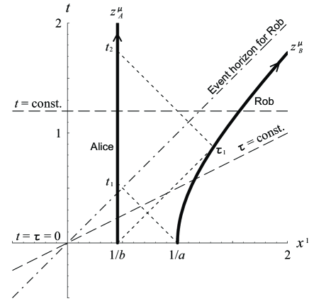
Figure 1: Alice is at rest along the world line $z_{A}^{\mu}(t)=(t,1/b,0,0)$ and Rob is uniformly accelerated along the trajectory $z_{B}^{\mu}(\tau)=(a^{-1}\sinh a\tau,a^{-1}\cosh a\tau,0,0)$, so the null hypersurface $t=x^{1}$ is Rob’s event horizon. The initial state of the combined system is defined on the hypersurface $t=\tau=0$, when the coupling between the detectors and the field is turned on. In this plot we choose $b=2.2$ and $a=1$ so $b>2a$.

Suppose the coupling between the detectors and the field is turned on at $t=\tau=0$, when the initial state of the combined system is a direct product of a quantum state $\left|\right.q_{A},q_{B}\left.\right>$ for Alice and Rob’s detectors $Q_{A}$ and $Q_{B}$ and the Minkowski vacuum $\left|\right.0_{M}\left.\right>$ for the field $\Phi$, namely,

$$\left|\right.\psi(0)\left.\right>=\left|\right.q_{A},q_{B}\left.\right>\otimes\left|\right.0_{M}\left.\right>.$$ (2)

Here $\left|\right.q_{A},q_{B}\left.\right>$ is taken to be a squeezed Gaussian state with minimal uncertainty, represented in the Wigner function as

$$\rho(Q_{A},P_{A},Q_{B},P_{B})={1\over\pi^{2}\hbar^{2}}\exp-{1\over 2}\left[{\beta^{2}\over\hbar^{2}}\left(Q_{A}+Q_{B}\right)^{2}+{1\over\alpha^{2}}\left(Q_{A}-Q_{B}\right)^{2}+{\alpha^{2}\over\hbar^{2}}\left(P_{A}-P_{B}\right)^{2}+{1\over\beta^{2}}\left(P_{A}+P_{B}\right)^{2}\right],$$ (3)

in which $Q_{A}$ and $Q_{B}$ can be entangled by properly choosing the parameters $\alpha$ and $\beta$.

Define the two-point correlation matrix $V$ with elements

$$V_{\mu\nu}(t,\tau)=\left<\right.{\cal R}_{\mu},{\cal R}_{\nu}\left.\right>\equiv{1\over 2}\left<\right.\left({\cal R}_{\mu}{\cal R}_{\nu}+{\cal R}_{\nu}{\cal R}_{\mu}\right)\left.\right>$$ (4)

where ${\cal R}_{\mu}=(Q_{B}(\tau),P_{B}(\tau),Q_{A}(t),P_{A}(t))$, $\mu,\nu=1,2,3,4$. The partial transpose of ${\bf V}$ is ${\bf V}^{PT}={\bf\Lambda V\Lambda}$, where ${\bf\Lambda}={\rm diag}(1,1,1,-1)$. Starting with the Gaussian initial state $(\ref{initGauss})$, the reduced density matrix or Wigner function of the two detectors is always Gaussian by virtue of the linearity of our model. Therefore Alice’s detector $Q_{A}$ and Rob’s detector $Q_{B}$ is entangled on time slice $t$ if and only if Si00

$$\Sigma(t,\tau=a^{-1}\sinh^{-1}at)\equiv\det\left[{\bf V}^{PT}+i{\hbar\over 2}{\bf M}\right]<0$$ (5)

where

$${\bf M}\equiv\left(\begin{array}[]{cccc}0&1&0&0\\ -1&0&0&0\\ 0&0&0&1\\ 0&0&-1&0\end{array}\right)$$ (6)

is a symplectic matrix. We find that when $\Sigma\leq 0$ the behavior of $\Sigma$ is quite similar to the behavior of the negative eigenvalues which are connected to the logarithm negativity VW02 . Thus the value of $\Sigma$ itself is a good indicator of the degree of entanglement, at least in this specific model. Since it is relatively easy to obtain the analytic form of $\Sigma(t)$ in the weak-coupling limit, we will calculate $\Sigma$ rather than the logarithm negativity to determine the disentanglement time analytically.

Below we calculate the two-point functions for matrix $V$. The uncertainty relation $\det[{\bf V}+i\hbar{\bf M}/2]\geq 0$ can serve as a double-check Si00 .

III Evolution of operators and correlators

III.1 Evolution of Operators

In the Heisenberg picture LH2005 ; LH2006 , the operators evolve as

$$\hat{Q}_{i}(\tau_{i}) = \sqrt{\hbar\over 2\Omega_{r}}\sum_{j}\left[q_{i}^{(j)}(\tau_{i})\hat{a}_{j}+q_{i}^{(j)*}(\tau_{i})\hat{a}_{j}^{\dagger}\right]+\int{d^{3}k\over(2\pi)^{3}}\sqrt{\hbar\over 2\omega}\left[q_{i}^{(+)}(\tau_{i},{\bf k})\hat{b}_{\bf k}+q_{i}^{(-)}(\tau_{i},{\bf k})\hat{b}_{\bf k}^{\dagger}\right],$$ (7)

$$\hat{\Phi}(x) = \sqrt{\hbar\over 2\Omega_{r}}\sum_{j}\left[f^{(j)}(x)\hat{a}_{j}+f^{(j)*}(x)\hat{a}_{j}^{\dagger}\right]+\int{d^{3}k\over(2\pi)^{3}}\sqrt{\hbar\over 2\omega}\left[f^{(+)}(x,{\bf k})\hat{b}_{\bf k}+f^{(-)}(x,{\bf k})\hat{b}_{\bf k}^{\dagger}\right],$$ (8)

with $i,j=A,B$, $\tau_{A}=t$, $\tau_{B}=\tau$. $q_{i}^{(j)}$, $q_{i}^{(\pm)}$, $f^{(j)}$ and $f^{(\pm)}$ are the (c-number) mode functions. The conjugate momenta are $\hat{P}_{A}(t)=\partial_{t}\hat{Q}_{A}(t)$, $\hat{P}_{B}(\tau)=\partial_{\tau}\hat{Q}_{B}(\tau)$, and $\hat{\Pi}(x)=\partial_{t}\hat{\Phi}(x)$. The Heisenberg equations of motion for operators imply

$$\left(\partial_{\tau_{i}}^{2}+\Omega_{0}^{2}\right)q_{i}^{(j)}(\tau_{i}) = \lambda_{0}f^{(j)}(z_{i}^{\mu}(\tau_{i})),$$ (9)

$$\left(\partial_{t}^{2}-\nabla^{2}\right)f^{(j)}(x) = \lambda_{0}\left[\int_{0}^{\infty}dt\,q_{A}^{(j)}\delta^{4}(x-z_{A}(t))+\int_{0}^{\infty}d\tau\,q_{B}^{(j)}\delta^{4}(x-z_{B}(\tau))\right],$$ (10)

$$\left(\partial_{\tau_{i}}^{2}+\Omega_{0}^{2}\right)q_{i}^{(+)}(\tau_{i},{\bf k}) = \lambda_{0}f^{(+)}(z_{i}^{\mu}(\tau_{i}),{\bf k}),$$ (11)

$$\left(\partial_{t}^{2}-\nabla^{2}\right)f^{(+)}(x,{\bf k}) = \lambda_{0}\left[\int_{0}^{\infty}dt\,q_{A}^{(+)}(t,{\bf k})\delta^{4}(x-z_{A}(t))+\int_{0}^{\infty}d\tau\,q_{B}^{(+)}(\tau,{\bf k})\delta^{4}(x-z_{B}(\tau))\right],$$ (12)

which have the same appearance as the corresponding classical dynamical equations. $f^{(j)}$ and $f^{(+)}$ look like classical fields generated by two pointlike sources at $z_{A}$ and $z_{B}$. Solving the field equations $(\ref{feAB1})$ and $(\ref{fe+1})$, one obtains $f^{(j)}$ and $f^{(+)}$ related to $q_{i}^{(j)}$ and $q_{i}^{(+)}$ by the retarded Green’s functions of the field. Inserting them into the equations of motion $(\ref{eomqAB1})$ and $(\ref{eomq+1})$ one obtains the solutions of $q_{i}^{(j)}$ and $q_{i}^{(+)}$. However, the self-field induced by $q_{i}^{(j)}$ and $q_{i}^{(+)}$ diverge at the positions of the two detectors, so one has to introduce cutoffs to handle them. Assuming Alice and Rob have the same frequency cutoffs in their local frame, one can do the same renormalization on frequency and obtain the effective equations of motion under the influence of field LH2005 :

$$\left(\partial_{t}^{2}+2\gamma\partial_{t}+\Omega_{r}^{2}\right)q_{A}^{(j)}(t) = {\lambda_{0}^{2}\over 2\pi}{\theta\left[\tau_{-}(z_{A}(t))\right]\over aX(z_{A}(t))}q_{B}^{(j)}\left(\tau_{-}(z_{A}^{\mu}(t))\right),$$ (13)

$$\left(\partial_{\tau}^{2}+2\gamma\partial_{\tau}+\Omega_{r}^{2}\right)q_{B}^{(j)}(\tau) = {\lambda_{0}^{2}\over 4\pi}{\theta\left[z_{B}^{0}(\tau)-R(z_{B}(\tau))\right]\over R(z_{B}(\tau))}q_{A}^{(j)}\left(z_{B}^{0}(\tau)-R(z_{B}(\tau))\right),$$ (14)

$$\left(\partial_{t}^{2}+2\gamma\partial_{t}+\Omega_{r}^{2}\right)q_{A}^{(+)}(t,{\bf k}) = \lambda_{0}f_{0}^{(+)}(z_{A}(t),{\bf k})+{\lambda_{0}^{2}\over 2\pi}{\theta\left[\tau_{-}(z_{A}(t))\right]\over aX(z_{A}(t))}q_{B}^{(+)}\left(\tau_{-}(z_{A}^{\mu}(t)),{\bf k}\right),$$ (15)

$$\left(\partial_{\tau}^{2}+2\gamma\partial_{\tau}+\Omega_{r}^{2}\right)q_{B}^{(+)}(\tau,{\bf k}) = \lambda_{0}f_{0}^{(+)}(z_{B}(\tau),{\bf k})+{\lambda_{0}^{2}\over 4\pi}{\theta\left[z_{B}^{0}(\tau)-R(z_{B}(\tau))\right]\over R(z_{B}(\tau))}q_{A}^{(+)}\left(z_{B}^{0}(\tau)-R(z_{B}(\tau)),{\bf k}\right),$$ (16)

where $\Omega_{r}\equiv\sqrt{\Omega^{2}+\gamma^{2}}$ is the renormalized frequency, $\gamma\equiv\lambda_{0}^{2}/8\pi$, and

$$f_{0}^{(+)}(x,{\bf k}) \equiv e^{-i\omega t+i{\bf k\cdot x}},$$ (17)

$$R(x) \equiv \sqrt{\left(x_{1}-b^{-1}\right)^{2}+\rho^{2}},$$ (18)

$$X(x) \equiv \sqrt{\left(-UV+\rho^{2}+a^{-2}\right)^{2}+4a^{-2}UV},$$ (19)

$$\tau_{-}(x) \equiv -{1\over a}\ln{a\over 2|V|}\left(X-UV+\rho^{2}+{1\over a^{2}}\right),$$ (20)

with $U=t-x_{1}$, $V=t+x_{1}$, $\omega=|{\bf k}|$, and $\rho^{2}=x_{2}^{2}+x_{3}^{2}$. Here one can see that $q_{A}$ and $q_{B}$ are causally linked.

The solutions of $q_{A}$ and $q_{B}$’s satisfying the initial conditions

$$f^{(+)}(0,{\bf x};{\bf k})=e^{i{\bf k\cdot x}},\;\;\;\partial_{t}f^{(+)}(0,{\bf x};{\bf k})=-i\omega e^{i{\bf k\cdot x}},$$ (21)

$$q_{A}^{(A)}(0)=q_{B}^{(B)}(0)=1,\;\;\;\partial_{t}{q}_{A}^{(A)}(0)=\partial_{\tau}{q}_{B}^{(B)}(0)=-i\Omega_{r},$$ (22)

and $f^{(j)}(0,{\bf x})=\partial_{t}f^{(j)}(0,{\bf x})=q_{j}^{(+)}(0;{\bf k})=\partial_{\tau_{j}}q_{j}^{(+)}(0;{\bf k})=q_{A}^{(B)}(0)=\partial_{t}{q}_{A}^{(B)}(0)=q_{B}^{(A)}(0)=\partial_{\tau}{q}_{B}^{(A)}(0)=0$, are listed in Appendix A.

III.2 Two-Point functions of detectors

When sandwiched by the initial state $(\ref{initstat})$, the two-point functions split into

$$\left<\right.{\cal R}_{\mu},{\cal R}_{\nu}\left.\right>=\left<\right.{\cal R}_{\mu},{\cal R}_{\nu}\left.\right>_{\rm v}+\left<\right.{\cal R}_{\mu},{\cal R}_{\nu}\left.\right>_{\rm a}$$ (23)

where

$$\left<\right.{\cal R}_{\mu},{\cal R}_{\nu}\left.\right>_{\rm v} = {1\over 2}\left<\right.0_{M}|\left({\cal R}_{\mu}{\cal R}_{\nu}+{\cal R}_{\nu}{\cal R}_{\mu}\right)|0_{M}\left.\right>$$ (24)

$$= {\rm Re}\int{\hbar d^{3}k\over(2\pi)^{3}2\omega}r_{\mu}^{(+)}(t_{\mu},{\bf k})r_{\nu}^{(-)}(t_{\nu},{\bf k}),$$

$$\left<\right.{\cal R}_{\mu},{\cal R}_{\nu}\left.\right>_{\rm a} = {1\over 2}\left<\right.q_{A},q_{B}|\left({\cal R}_{\mu}{\cal R}_{\nu}+{\cal R}_{\nu}{\cal R}_{\mu}\right)|q_{A},q_{B}\left.\right>$$ (25)

$$= {1\over 4}\left\{\hbar^{2}\beta^{-2}{\rm Re}\left(r_{\mu}^{(A)}+r_{\mu}^{(B)}\right){\rm Re}\left(r_{\nu}^{(A)}+r_{\nu}^{(B)}\right)+\alpha^{2}{\rm Re}\left(r_{\mu}^{(A)}-r_{\mu}^{(B)}\right){\rm Re}\left(r_{\nu}^{(A)}-r_{\nu}^{(B)}\right)+\right.$$

$$\left.\Omega_{r}^{-2}\left[\beta^{2}{\rm Im}\left(r_{\mu}^{(A)}+r_{\mu}^{(B)}\right){\rm Im}\left(r_{\nu}^{(A)}+r_{\nu}^{(B)}\right)+\hbar^{2}\alpha^{-2}{\rm Im}\left(r_{\mu}^{(A)}-r_{\mu}^{(B)}\right){\rm Im}\left(r_{\nu}^{(A)}-r_{\nu}^{(B)}\right)\right]\right\},$$

where $r_{\mu}^{(j)}=(q_{B}^{(j)},p_{B}^{(j)},q_{A}^{(j)},p_{A}^{(j)})$ and $p_{i}^{(j)}=\partial_{\tau_{i}}q_{i}^{(j)}$. Substituting Eqs. $(\ref{qAA})$-$(\ref{qBp})$, one obtains the above two-point functions straightforwardly. The only complication is that the integration over $k$ space in (24) may diverge, so one has to introduce additional frequency cutoffs corresponding to the time-resolution of the detector ($\Lambda_{1}$) and the time scale of switching on the interaction ($\Lambda_{0}$) LH2005 ; LH2006 . After doing this, one has, for example,

$$\left<\right.Q_{B}^{2}(\tau)\left.\right>_{\rm v}=\left<\right.Q_{B}^{2}(\tau)\left.\right>_{\rm v}^{(0)}+\theta\left(\tau-\tau_{1}\right)\left<\right.Q_{B}^{2}(\tau)\left.\right>_{\rm v}^{(1)},$$ (26)

where $\tau_{1}\equiv a^{-1}\ln(b/a)$ (see Fig. 1), $\left<\right.Q_{B}^{2}\left.\right>_{\rm v}^{(0)}$ is the two-point function of a single uniformly accelerated detector (expressions of $\left<\right.Q_{B}^{2}\left.\right>_{\rm v}^{(0)}$, $\left<\right.P_{B}^{2}\left.\right>_{\rm v}^{(0)}$, $\left<\right.Q_{A}^{2}\left.\right>_{\rm v}^{(0)}$ and $\left<\right.Q_{B}^{2}\left.\right>_{\rm v}^{(0)}$ have been listed in Appendix A of Ref. LH2006 ), while the higher order correction reads

$$\left<\right.Q_{B}^{2}(\tau)\left.\right>_{\rm v}^{(1)} = {4\gamma\over\Omega}\int_{\tau_{1}}^{\tau}d\tau^{\prime}{e^{-r(\tau-\tau^{\prime})}\sin\Omega(\tau-\tau^{\prime})\over{1\over a}\cosh a\tau^{\prime}-{1\over b}}\left<\right.Q_{B}(\tau),Q_{A}(b^{-1}-a^{-1}e^{-a\tau^{\prime}})\left.\right>_{\rm v}^{(0)}$$ (27)

$$+ {4\gamma^{2}\over\Omega^{2}}\int_{\tau_{1}}^{\tau}d\tau^{\prime}{e^{-r(\tau-\tau^{\prime})}\sin\Omega(\tau-\tau^{\prime})\over{1\over a}\cosh a\tau^{\prime}-{1\over b}}\int_{\tau_{1}}^{\tau}d\tau^{\prime\prime}{e^{-r(\tau-\tau^{\prime\prime})}\sin\Omega(\tau-\tau^{\prime\prime})\over{1\over a}\cosh a\tau^{\prime\prime}-{1\over b}}\times$$

$$\,\,\,\,\,\,\,\,\,\,\left<\right.Q_{A}(b^{-1}-a^{-1}e^{-a\tau^{\prime}}),Q_{A}(b^{-1}-a^{-1}e^{-a\tau^{\prime\prime}})\left.\right>_{\rm v}^{(0)}.$$

Calculating the cross correlations $\left<\right.{\cal R}_{A}(t),{\cal R}_{B}(\tau)\left.\right>_{\rm v}^{(0)}$ (${\cal R}=P,Q$) is also straightforward, though one has to be careful about the contours of integration of each term on the complex plane of $\kappa$ (see LH2005 ). Note that $\Lambda_{1}$ is present only in $\left<\right.P_{A}^{2}\left.\right>_{\rm v}$ and $\left<\right.P_{B}^{2}\left.\right>_{\rm v}$.

IV Disentanglement dynamics

IV.1 ultraweak-coupling limit

In the ultraweak-coupling limit ($\gamma\Lambda_{1}\ll a,\Omega$), the corrections due to the retarded mutual influences in mode functions $(\ref{qAA})$-$(\ref{qBp})$ are $O(\gamma)$ and suppressed, while the cross correlations $\left<\right.{\cal R}_{A},{\cal R}_{B}\left.\right>_{\rm v}$ (${\cal R}=P,Q$) accounting for the response to the vacuum fluctuations are negligible. The two-point functions $\left<\right...\left.\right>_{\rm a}$ behave like $(\ref{Qj2aweak})$-$(\ref{QAPBaweak})$, and

$$\left<\right.Q_{A}^{2}(t)\left.\right>_{\rm v} \approx {\hbar\over 2\Omega}\left(1-e^{-2\gamma t}\right),$$ (28)

$$\left<\right.Q_{B}^{2}(\tau)\left.\right>_{\rm v} \approx {\hbar\over 2\Omega}\coth{\pi\Omega\over a}\left(1-e^{-2\gamma\tau}\right),$$ (29)

and $\left<\right.P_{j}^{2}(\tau_{j})\left.\right>_{\rm v}\approx\Omega^{2}\left<\right.Q_{j}^{2}(\tau_{j})\left.\right>_{\rm v}$, $j=A,B$. It is straightforward to calculate $\Sigma$ and determine the separability of Alice and Rob by inserting these two-point functions into (5).

IV.1.1 Evolution of entanglement in Alice’s proper time (Minkowski time)

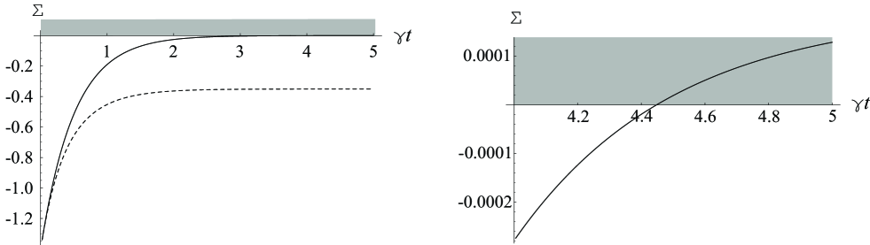
Figure 2: (Left) The behavior of $\Sigma$ (solid curve) defined in $(\ref{Entcond})$ can be approximated by $(\ref{Siga})$ in the ultraweak-coupling limit with $a$ sufficiently large. Two detectors are separable when $\Sigma\geq 0$ (shaded zone), otherwise entangled. Here $\gamma=10^{-5}$, $a=0.1$, $b=0.201$, $\alpha=1.1$, $\beta=4.5$, $\Lambda_{0}=\Lambda_{1}=100$, $\Omega=2.3$ and $\hbar=1$. By comparison the dotted curve is $\Sigma$ with all $\left<\right...\left.\right>_{\rm v}$ set to be zero. Both curves will become positive at late times. (Right) Looking more closely, one finds that two detectors are separable, or totally disentangled, after $\gamma t\approx 4.44$.

At the initial moment $t=0$, the initial Gaussian state $(\ref{initGauss})$ has

$$\Sigma\approx-{\hbar^{2}\over 16\alpha^{2}\beta^{2}}\left(\hbar^{2}-\alpha^{2}\beta^{2}\right)^{2}.$$ (30)

Thus for all $\alpha^{2}\beta^{2}\not=\hbar^{2}$, two detectors are entangled. Below we will see that quantum entanglement will, however, vanish at a finite disentanglement time (“sudden death”), which is usually different from the decoherence time scale $\gamma^{-1}$.

For proper acceleration $a$ sufficiently large such that $\tau=a^{-1}\sinh^{-1}at\ll t$ for $t$ large enough, one has $e^{\gamma(t+\tau)}\approx e^{\gamma t}$ and

$$\Sigma\approx-{\hbar^{2}\over 16\alpha^{2}\beta^{2}}\left(\hbar^{2}-\alpha^{2}\beta^{2}\right)^{2}e^{-2\gamma t}.$$ (31)

An example is illustrated in Fig. 2. The disentanglement time of this case looks infinite. However, the correction of the next order will shift the curve of $\Sigma$ upward and make the disentanglement time finite. When $\Lambda_{1}$ is large, such a correction is dominated by $\Lambda_{1}$ terms in $\left<\right.P_{j}^{2}\left.\right>_{\rm v}$:

$$\left<\right.P_{A}^{2}\left.\right>_{\rm v} \approx {\hbar\over 2}\Omega\left(1-e^{-2\gamma t}\right)+{2\over\pi}\hbar\gamma\Lambda_{1},$$ (32)

$$\left<\right.P_{B}^{2}\left.\right>_{\rm v} \approx {\hbar\over 2}\Omega\coth{\pi\Omega\over a}\left(1-e^{-2\gamma\tau}\right)+{2\over\pi}\hbar\gamma\Lambda_{1}$$ (33)

[see Eqs.(A4) and (A10) in Ref.LH2006 ]. For $t_{dE}\gg 1$, this correction yields

$$\Sigma\approx-{\hbar^{2}\over 16\alpha^{2}\beta^{2}}\left(\hbar^{2}-\alpha^{2}\beta^{2}\right)^{2}e^{-2\gamma t}+{\hbar^{2}\gamma\Lambda_{1}\over 16\pi\alpha^{2}\beta^{2}}\left(\hbar^{2}-\alpha^{2}\beta^{2}\right)^{2},$$ (34)

around $t\approx t_{dE}$, which gives

$$t_{dE}\approx{1\over 2\gamma}\ln{\pi\Omega\over\gamma\Lambda_{1}}.$$ (35)

In Fig.2, one has $\gamma t_{dE}\approx 4.44$.

Note that $\Sigma$ is insensitive to $a$ here. This implies that, to leading order in the ultraweak-coupling approximation, Unruh effect does little to the disentanglement between Alice and Rob from the view of Alice.

IV.1.2 Two inertial detectors in Minkowski vacuum

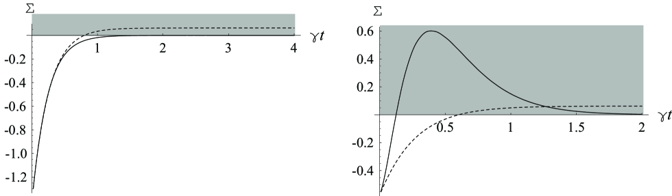
Figure 3: When $a\to 0$, the behavior of $\Sigma$ in the weak-coupling limit can be described by $(\ref{Sig0})$. Here $(\alpha,\beta)=(1.1,4.5)$ for the left plot ($Z_{4}<0$) and $(1.5,0.2)$ for the right plot ($Z_{4}>0$). The solid curves represent $\Sigma$ in its totality, while the dotted curves represent $\Sigma$ with all $\left<\right...\left.\right>_{\rm v}$ set to be zero.

For $a\to 0$, $\coth(\pi\Omega/a)\to 1$, $\tau\to t$, and Rob is also inertial. Suppose Alice and Rob are separated far enough, so the mutual influences can be safely ignored again. Then, in the weak-coupling limit with $\Omega\gg\gamma\Lambda_{1}\gg a\to 0$, one has

$$\Sigma\approx{\hbar^{2}e^{-4\gamma t}\over 16\alpha^{2}\beta^{2}\Omega^{2}}\left[Z_{8}\left(e^{-4\gamma t}-2e^{-2\gamma t}\right)+Z_{4}\right],$$ (36)

where

$$Z_{8} \equiv \left(\hbar-\alpha^{2}\Omega\right)^{2}\left(\beta^{2}-\hbar\Omega\right)^{2},$$ (37)

$$Z_{4} \equiv \hbar^{2}\left(\beta^{4}+\alpha^{4}\Omega^{4}+6\alpha^{2}\beta^{2}\Omega^{2}\right)-2\hbar\Omega\left(\beta^{2}+\alpha^{2}\Omega^{2}\right)\left(\hbar^{2}+\alpha^{2}\beta^{2}\right).$$ (38)

It is clear that $Z_{8}\geq 0$ and $Z_{8}-Z_{4}\geq 0$. When $Z_{4}>0$, the disentanglement time is clearly finite:

$$t_{dE}\approx-{1\over 2\gamma}\ln\left(1-\sqrt{1-{Z_{4}\over Z_{8}}}\right).$$ (39)

Indeed, one has $\gamma t_{dE}\approx 0.125$ in the right plot of Fig. 3.

When $Z_{4}<0$, the disentanglement time looks infinite. But again, the corrections of the next order yields

$$\Sigma\approx{\hbar^{2}\over 16\alpha^{2}\beta^{2}\Omega^{2}}Z_{4}e^{-4\gamma t}+{\hbar^{3}\gamma\Lambda_{1}\over 4\pi\alpha^{2}\beta^{2}\Omega^{2}}Z_{2}e^{-2\gamma t}+{\hbar^{4}\over\pi^{2}\Omega^{2}}\gamma^{2}\Lambda_{1}^{2}$$ (40)

around $t\approx t_{dE}\gg 1$ for large $\Lambda_{1}$, with

$$Z_{2}\equiv\alpha^{2}\left(\beta^{2}-\hbar\Omega\right)^{2}+\beta^{2}\left(\alpha^{2}\Omega-\hbar\right)^{2}\geq 0.$$ (41)

This gives a finite disentanglement time

$$t_{dE}\approx{1\over 2\gamma}\ln{|Z_{4}|\pi/(2\hbar\gamma\Lambda_{1})\over Z_{2}+\sqrt{Z_{2}^{2}-4\alpha^{2}\beta^{2}Z_{4}}},$$ (42)

and $\gamma t_{dE}\approx 3.96$ in Fig. 3 (left).

The dotted curves in Figs. 2 (left) and 3 (left and right) are those $\Sigma$s with vacuum fluctuations of the field switched off, namely, with $\left<\right.{\cal R}_{\mu},{\cal R}_{\nu}\left.\right>_{\rm v}$ set to be zero. In Fig. 2 (left) it seems that vacuum fluctuations would reduce $|\Sigma|$ thus suppressing the entanglement. This is not true. One can verify that, for sufficiently large $t$, the dashed curve in Figs. 2 (left) will overtake the solid curve and then become positive, just like what Fig. 3 (right) suggests. In the weak-coupling limit, the vacuum fluctuations of the field that the detectors see locally do not always suppress (or enhance) quantum entanglement beyond the disentanglement due to the dissipation of initial quantum fluctuations of the detectors (corresponding to the exponential decay of $\left<\right...\left.\right>_{\rm a}$ in time.)

IV.1.3 Evolution of entanglement in Rob’s proper time (Rindler time)

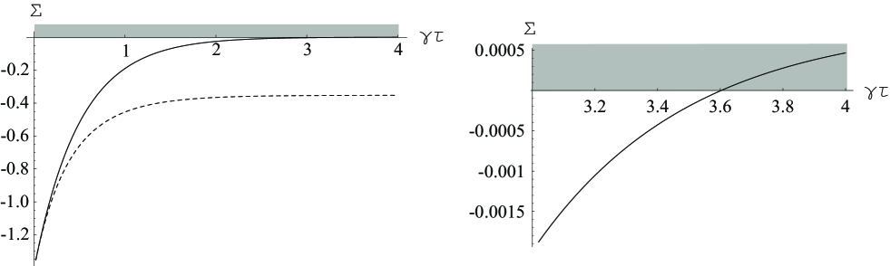
Figure 4: The solid curves represent $\Sigma$ in its totality in Rob’s point of view. “Sudden death” of entanglement occurs at $\gamma\tau_{dE}\approx 3.61$, as can be seen in the enlargement on the right plot. The dotted curve represents $\Sigma$ with all $\left<\right...\left.\right>_{\rm v}$ set to be zero. All parameters are the same as those in Fig. 2 except $\gamma=10^{-6}$, $a=2$ and $b=4.1$.

The hypersurface with constant Rindler time $\tau$ extends to $t<0$ region in the left half of the Minkowski space (see Fig.1). Suppose, even before the initial time slice with $t=0$, the field state has been the Minkowski vacuum. Then the field state in Rindler time slicing is also a Gaussian state and the quantity $\Sigma(t,\tau)$, with a similar definition to $(\ref{Entcond})$ but we let $t=b^{-1}\tanh a\tau$ here, can still serve as an measure of the entanglement between Alice’s and Rob’s detector in Rob’s frame.

For $a$ sufficiently large, $\gamma t\to\gamma/b\ll 1$ for large $\tau$. Then

$$\Sigma(t=b^{-1}\tanh a\tau,\tau)\approx{\hbar^{2}\over 64\alpha^{2}\beta^{2}}\left(\hbar^{2}-\alpha^{2}\beta^{2}\right)^{2}\left[\left(1-e^{-2\gamma\tau}\right)^{2}\coth^{2}{\pi\Omega\over a}-\left(1+e^{-2\gamma\tau}\right)^{2}\right],$$ (43)

and the disentanglement time is approximately

$$\tau_{dE}\approx{\pi\Omega\over\gamma a},$$ (44)

in Rob’s point of view (see Fig. 4). This result may be interpreted as presenting a dynamical version of the statement “quantum entanglement is degraded in noninertial frames” AM03 ; FSM05 . Note that in Rob’s frame Alice will never cross the event horizon. So the quantum entanglement here is not the one “across the event horizon”.

When $a$ gets smaller, $\Sigma$ approaches those described in the previous subsections. When $a\to 0$, the value of the finite disentanglement time recovers the disentanglement time in the case of two inertial detectors.

IV.2 Beyond the ultraweak-coupling limit

IV.2.1 High acceleration regime

When the proper acceleration of Rob is very large, Rob will reach a very high speed in a very short time, when the time dilation makes Rob appear almost frozen in the view of Alice, and the disentanglement process becomes slower than those in the case with Rob’s acceleration smaller. In other words, in our setup, the larger acceleration Rob has, the longer the disentanglement time in Alice’s clock (see Fig. 5), while in Rob’s frame $\tau_{dE}$ is shorter from $(\ref{tdERob})$. The statement “a state which is maximally entangled in an inertial frame becomes less entangled if the observers are relatively accelerated” FSM05 is too simplistic and could be misleading here.

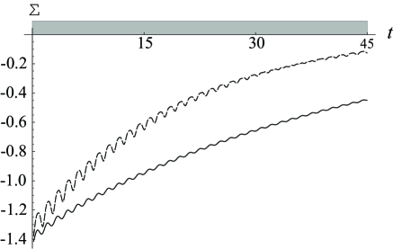
Figure 5: $\Sigma$ for Rob in high acceleration (solid curve) with $a=10$ and $b=21$. ($a=.01$, $b=.021$ for the dashed curve for comparison.) The large time dilation makes Rob appear almost frozen in the view of Alice at large $t$, and the disentanglement time is longer for larger $a$. Here $\gamma=0.01$, $\Lambda_{0}=\Lambda_{1}=50$, and other parameters are the same as those in Fig. 2.

IV.2.2 strong-coupling regime

When the coupling becomes larger, there will be oscillation emerging on top of the smooth curve of $\Sigma$ in the ultraweak-coupling limit. So around $t_{dE}$ the entanglement between the detectors of Alice and Rob may disappear and revive for several times, before they finally become separable forever. The duration of such kind of entanglement revival will not exceed the order of time scale $1/\Omega$ (see the upper plot of Fig. 8.)

When the coupling gets even larger, the vacuum fluctuations will exert a strong impact on quantum entanglement. Usually this shortens the disentanglement time. Indeed, in Fig. 6 we find that, for $\gamma\Lambda_{1}$ sufficiently large, the initial quantum entanglement is annulled right after the coupling is switched on.

The higher order corrections to $\Sigma$ from retarded mutual influences of two detectors, while their amplitudes decay in time, are not always positive or negative. Nevertheless, the memory effect induced by mutual influences contributes little in the cases considered: Although the total corrections to $\Sigma$ from mutual influences become more obvious for a larger coupling, they are of $O(\gamma^{2})$ and remain small as seen in Fig. 6. Results with stronger mutual influences will be reported in a future work.

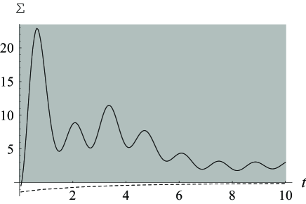
Figure 6: $\Sigma$ in the strong-coupling regime. The entanglement between Alice and Rob in their initial state is annulled by the strong impact of vacuum fluctuations ($\Sigma>0$) right after the coupling is switched on. Here $\gamma=0.1$, $\Lambda_{0}=\Lambda_{1}=50$, $a=1$, $b=2.01$, and other parameters are the same as those in Fig. 2. The dotted curve at the bottom are the $\Sigma$ with all $\left<\right...\left.\right>_{\rm v}$ turned off. Numerically we find that the higher order corrections to $\Sigma$ from mutual influences are less than $2\%\sim O(\gamma^{2})$.

V Discussion

V.1 Infinite disentanglement time in Markovian limit

A criterion in the Markovian limit on finite disentanglement time has been offered by Yu and Eberly YE04 . In some parameter range ($a\in(0,1/3)$ there) the concurrence decays exponentially in time so the disentanglement time looks infinite. Here we have similar situations in the ultraweak-coupling limit as discussed in Secs. IV.1.1 and IV.1.2. In particular, the parameter $Z_{4}$ in $(\ref{Sig0})$ plays an analogous role to $a$ in YE04 . While the entanglement gets a clear sudden death when $Z_{4}>0$, the disentanglement time looks infinite otherwise. However, in Secs. IV.1.1 and IV.1.2 we showed that the correction from the next order to the ultraweak-coupling approximation will render the disentanglement time of the latter case finite. According to our results, it will be interesting to see whether the infinite disentanglement time in the Markovian cases that Yu and Eberly considered would become finite if one considers the corrections beyond the Markovian approximation.

V.2 Entanglement and correlation

When cross correlations vanish, two detectors are uncorrelated and the two-point correlation matrix ${\bf V}$ defined in $(\ref{CorrMtx})$ is block diagonalized so the Wigner function, or the reduced density matrix, for the detectors can be factorized into a tensor product of two Wigner functions or reduced density matrices for each detector. Now two detectors are simply separable, with a stronger condition than those for disentangled or separable states.

In our model, the cross correlations $\left<\right.{\cal R}_{A},{\cal R}_{B}\left.\right>$ always vanish as $\gamma t\to\infty$, while the two-point functions of each detector remain finite. We found $|\left<\right.{\cal R}_{A},{\cal R}_{B}\left.\right>|\sim e^{-\epsilon t}$ with $\epsilon\propto\gamma$ at sufficiently large $t$. This implies that there is no residual entanglement at late times because

$$\Sigma|_{\gamma t\to\infty}=\left.\left[\left<\right.Q_{A}^{2}\left.\right>^{(0)}\left<\right.P_{A}^{2}\left.\right>^{(0)}-{\hbar^{2}\over 4}\right]\left[\left<\right.Q_{B}^{2}\left.\right>^{(0)}\left<\right.P_{B}^{2}\left.\right>^{(0)}-{\hbar^{2}\over 4}\right]\right|_{\gamma t\to\infty},$$ (45)

which is a product of the uncertainty relations for each detector in steady state and is positive-definite if the coupling $\lambda_{0}$ is nonvanishing. (Note that $\left<\right.Q_{A},P_{A}\left.\right>\sim e^{-\gamma t}$ and $\left<\right.Q_{B},P_{B}\left.\right>\sim\exp[-(a+\gamma)a^{-1}\sinh^{-1}at]$ vanish at late times; for explicit expressions of other late-time two-point functions, see Appendix A in Ref. LH2006 .) In Minkowski time, two detectors become separable after a finite disentanglement time $t_{dE}$, but not simply separable or uncorrelated until $\gamma t\to\infty$.

V.3 time slicing and coordinate dependence

Consider two events, one in Alice’s world line at her proper time $t=\bar{t}$, the other in Rob’s world line at his proper time $\tau=\bar{\tau}$, defined on the same time slice in some coordinate. Recall that the physical RDM for the two detectors are obtained by integrating out the degrees of freedom of the field defined on the same hypersurface associated with a certain time slicing. Thus the RDM of the two detectors at the two events $z^{\mu}_{A}(\bar{t})$ and $z^{\mu}_{B}(\bar{\tau})$ should always be associated with a specification of a time slicing scheme, so should the criterion of separability derived from the RDM. But there are infinitely many choices of time slices intersecting Alice and Rob’s world line right at these two events. Does quantum entanglement of the detectors at $z^{\mu}_{A}(\bar{t})$ and $z^{\mu}_{B}(\bar{\tau})$ depend on different choices of time slice?

In the cases we considered in this paper, the answer is no. In our UD detector theory, the coordinate transformation from Minkowski coordinate to a new coordinate consistent with some other time slicing scheme such as Rindler time will not change the quadratic form of the action $(\ref{Stot1})$, so the combined system in the new coordinate is still linear. If the initial time slice in the new time slicing scheme is identical to our $t=0$ hypersurface in Minkowski coordinate, and the combined system is starting with a Gaussian initial state such as $(\ref{initstat})$, the quantum state of the combined system will remain Gaussian during the evolution in the new time slicing scheme. Hence the RDM of the detectors is still Gaussian and the criterion $(\ref{Entcond})$ can be applied in this new time slicing. The Gaussianity implies that both the RDM of the detectors and the criterion $(\ref{Entcond})$ are fully described by the two-point functions of the detectors $\left<\right.{\cal R}_{\mu},{\cal R}_{\nu}\left.\right>$, which are independent of the choice of time slice connecting these two events. Thus the RDM and the separability of the Gaussian state at those two events are independent of time slicing. We believe that this is a general feature of quantum entanglement in relativistic quantum information theory.

Nevertheless, in Secs.IV.1.1 and IV.1.3 we learnt that the entanglement dynamics and the disentanglement (proper) time are coordinate-dependent, because in general two events simultaneous in one (e.g. Minkowski) coordinate are not simultaneous in another (e.g. Rindler) coordinate, while quantum entanglement is a property of a quantum state of two events at the same time slice.

V.4 Detector-detector entanglement vs detector-field entanglement

Quantum coherence in a detector is related to its purity, which also indicates the degree of quantum entanglement between that detector and the rest of the combined system (the field and the other detector)BZ06 . Since the combined system is a Gaussian state, the reduced density matrix for each detector is also Gaussian. So the purities of Alice and Rob’s detectors are simply LH2006

$${\cal P}_{j}={\hbar/2\over\sqrt{\left<\right.P_{j}^{2}\left.\right>\left<\right.Q_{j}^{2}\left.\right>-\left<\right.P_{j},Q_{j}\left.\right>^{2}}},$$ (46)

where $j=A,B$. Obviously the information contained in the cross correlations $\left<\right.{\cal R}_{A},{\cal R}_{B}\left.\right>$ is ignored in every combination of ${\cal P}_{j}$. We illustrate some examples in Fig. 7. One can see that the evolution of purity in each detector is quite different from the evolution of entanglement between them. There is no “sudden death” of quantum entanglement between one detector and the rest, and the late-time purity is always less than one. This is a consequence of the direct interaction between each detector and the field.

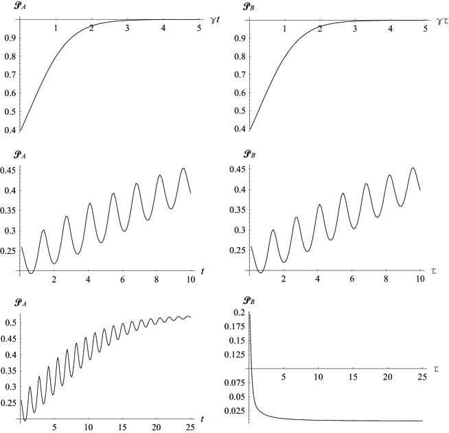
Figure 7: Purities of Alice (${\cal P}_{A}$) and Rob (${\cal P}_{B}$). (Top) ${\cal P}_{A}$ and ${\cal P}_{B}$ in the ultraweak-coupling regime, with the same parameters as those in Fig. 2. In this regime ${\cal P}_{A}$ and ${\cal P}_{B}$ each in its own proper time has virtually the same behavior. (Middle) ${\cal P}_{A}$ and ${\cal P}_{B}$ in the strong-coupling regime, with the same parameters as those in Fig. 6. Again their difference is very tiny. (Bottom) ${\cal P}_{A}$ and ${\cal P}_{B}$ in high acceleration limit, with the same parameters as those for the solid curve in Fig. 5. Now their difference is evident.

V.5 Disentanglement time and separation of detectors

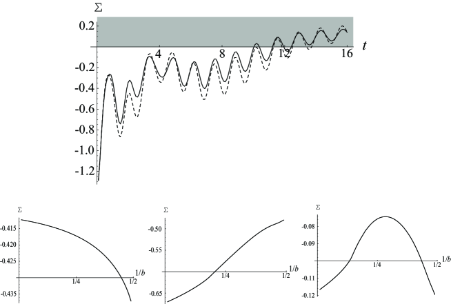
Figure 8: (Upper) $\Sigma$ with initial separation $d_{I}\approx 0.5025$ ($b=2.01$) for the solid curve and $d_{I}=0.9999$ ($b=10000$) for the dashed curve. Alice is located at $z_{A}^{1}=1/b$ and the initial separation between Alice and Rob at $t=0$ is $d_{I}=a^{-1}-b^{-1}$. Here $a=1$, $\gamma=0.025$, $\Lambda_{0}=\Lambda_{1}=50$, and other parameters are the same as those in Fig. 2. One can see that short-time revivals of entanglement occur during $t\approx 10\sim 11$ and around $t=12$. (Lower) The dependence of $\Sigma$ on the initial separation is not evident systematically: from left to right are $\Sigma$ at $t=0.5,2.5,3.2$, respectively.

Naively one may think that spatially the closer Alice and Bob are, the larger $\left<\right.{\cal R}_{A},{\cal R}_{B}\left.\right>$, so the disentanglement time gets shorter. Our results in Fig. 8 show that this is not true. One can hardly see any simple relation between the initial separation of the two detectors and the disentanglement time. The larger the separation, the stronger the entanglement ($\Sigma$ more negative) at some moments, but weaker at others.

We have considered the case with both detectors being at rest and spatially separated. While the higher order corrections from mutual influences are complicated and quite hard to handle as $t$ increases, for separation $d$ large enough that the mutual influences cannot reach in time (namely, $d>ct$), we get a similar result that no simple proportionality exists between the separation and the degree of entanglement of the two detectors. As the system evolves, sometimes the entanglement is stronger for larger separation, sometimes it is weaker.

V.6 How generic are the features contained in this model?

Our results show that the disentanglement time in our model is finite in all cases considered. But how generic are these results?

Our model has two UD detectors spatially separated in (3+1)D spacetime, one stationary and another uniformly accelerating and running away, without any direct interaction with each other. The presence of the event horizon for Rob has the effect of curtailing the mutual influences higher than a certain order. When we focus on one single UD detector, it behaves like the QBM of a harmonic oscillator interacting with an Ohmic bath provided by the (3+1)D scalar quantum field HM94 .

If there exists a direct interaction between the two detectors, there will certainly be residual entanglement between them at late times, just like the late-time entanglement between each detector and the field in our model.

The scalar field in our model is living in a free space. The presence of boundaries will change the result. The backreaction started from each detector when reflected by boundaries will add another memory effect to the dynamics of entanglement and affect the late-time behavior of detectors. One example is an electromagnetic field in a perfect cavity. Spacetime dimension also matters. Different spacetime dimensions or boundaries give different spectral density functions of the field experienced by the detectors HM94 . Moreover, in $(n+1)$D, $n\geq 3$ the spatial separation $d$ implies a suppression of mutual influences by a factor $1/d^{n-2}$, so the mutual influences would be negligible in the cases with large spatial separation.

Spatial separation also contributes to the retardation of mutual influences, and since Alice is at rest and Rob is in uniform acceleration, one detector’s dynamics is generally out of phase from the backreaction of the other. If the two detectors are located very close to each other through the whole dynamical process, or the two detectors are separated at a distance where resonance ($d\approx 2\pi c/\Omega$) is set up, the features of the disentanglement process can be different. For example, residual entanglement at late times under specific conditions in the 2HO QBM model has been reported in PR07 ; AZ07 ; that model is equivalent to a detector theory with two UD detectors sitting at the same point in 3D space, when the HO bath is ohmic.

Therefore, we believe that our results in this paper are generic for two well-separated detectors or atoms without direct interaction with each other, but coupled to a common quantum field in $(n+1)$D, $(n\geq 3)$ Minkowski space without boundary.

Acknowledgement SYL wishes to thank Jun-Hong An for illuminating discussions, and David Ostapchuk for finding a small localized mistake in the calculation reported in the first version which does not affect any claims or results reported. BLH and SYL thank Rafael Sorkin for a useful comment on the dependence of the Gaussianity of a state on slicing. This work is supported in part by NSF Grants No. PHY-0601550 and No. PHY-0426696.

Appendix A Expressions for mode functions

For the cases with $b>2a$, one has

$$q_{A}^{(A)}(t)=\theta(t){e^{-\gamma t}\over 2}\left[W_{-}e^{i\Omega t}+W_{+}e^{-i\Omega t}\right]$$

$$\,\,\,+{\theta\left(t-t_{2}\right)\lambda_{0}^{4}\over 16\pi^{2}a\Omega^{2}}\int^{t}_{t_{2}}{dt^{\prime}K(t-t^{\prime})\over t^{\prime 2}-b^{-2}+a^{-2}}\int^{\tau_{-}(t^{\prime})}_{\tau_{1}}{d\tau^{\prime}K[\tau_{-}(t^{\prime})-\tau^{\prime}]\over a^{-1}\cosh a\tau^{\prime}-b^{-1}}e^{-\gamma t_{-}(\tau^{\prime})}\left[W_{-}e^{i\Omega t_{-}(\tau^{\prime})}+W_{+}e^{-i\Omega t_{-}(\tau^{\prime})}\right],$$ (47)

$$q_{B}^{(A)}(\tau)=\theta\left(\tau-\tau_{1}\right){\lambda_{0}^{2}\over 8\pi\Omega}\int^{\tau}_{\tau_{1}}{d\tau^{\prime}K(\tau-\tau^{\prime})\over a^{-1}\cosh a\tau^{\prime}-b^{-1}}e^{-\gamma t_{-}(\tau^{\prime})}\left[W_{-}e^{i\Omega t_{-}(\tau^{\prime})}+W_{+}e^{-i\Omega t_{-}(\tau^{\prime})}\right],$$ (48)

$$q_{A}^{(B)}(t)=\theta\left(t-t_{1}\right){\lambda_{0}^{2}\over 4\pi a\Omega}\int^{t}_{t_{1}}{dt^{\prime}K(t-t^{\prime})\over t^{\prime 2}-b^{-2}+a^{-2}}e^{-\gamma\tau_{-}(t^{\prime})}\left[W_{-}e^{i\Omega\tau_{-}(t^{\prime})}+W_{+}e^{-i\Omega\tau_{-}(t^{\prime})}\right],$$ (49)

$$q_{B}^{(B)}(\tau)=\theta(\tau){e^{-\gamma\tau}\over 2}\left[W_{-}e^{i\Omega\tau}+W_{+}e^{-i\Omega\tau}\right],$$ (50)

$$q_{A}^{(+)}(t,{\bf k})=\theta(t){\lambda_{0}\over\Omega}\int_{0}^{t}dt^{\prime}K(t-t^{\prime})f_{0}^{(+)}(z_{A}(t^{\prime}),{\bf k})$$

$$\,\,\,+\theta\left(t-t_{1}\right){\lambda_{0}^{3}\over 2\pi a\Omega^{2}}\int^{t}_{t_{1}}{dt^{\prime}K(t-t^{\prime})\over t^{\prime 2}-b^{-2}+a^{-2}}\int_{0}^{\tau_{-}(t^{\prime})}d\tau^{\prime}K[\tau_{-}(t^{\prime})-\tau^{\prime}]f_{0}^{(+)}(z_{B}(\tau^{\prime}),{\bf k})$$

$$\,\,\,+{\theta\left(t-t_{2}\right)\lambda_{0}^{5}\over 8\pi^{2}a\Omega^{3}}\int^{t}_{t_{2}}{dt^{\prime}K(t-t^{\prime})\over t^{\prime 2}-b^{-2}+a^{-2}}\int^{\tau_{-}(t^{\prime})}_{\tau_{1}}{d\tau^{\prime}K[\tau_{-}(t^{\prime})-\tau^{\prime}]\over a^{-1}\cosh a\tau^{\prime}-b^{-1}}\int_{0}^{t_{-}(\tau^{\prime})}dt^{\prime\prime}K[t_{-}(\tau^{\prime})-t^{\prime\prime}]f_{0}^{(+)}(z_{A}(t^{\prime\prime}),{\bf k}),$$ (51)

$$q_{B}^{(+)}(\tau,{\bf k})=\theta(\tau){\lambda_{0}\over\Omega}\int_{0}^{\tau}d\tau^{\prime}K(\tau-\tau^{\prime})f_{0}^{(+)}(z_{B}(\tau^{\prime}),{\bf k})$$

$$\,\,\,+\theta\left(\tau-\tau_{1}\right){\lambda_{0}^{3}\over 4\pi\Omega^{2}}\int^{\tau}_{\tau_{1}}{d\tau^{\prime}K(\tau-\tau^{\prime})\over a^{-1}\cosh a\tau^{\prime}-b^{-1}}\int_{0}^{t_{-}(\tau^{\prime})}dt^{\prime}K[t_{-}(\tau^{\prime})-t^{\prime}]f_{0}^{(+)}(z_{A}(t^{\prime}),{\bf k}).$$ (52)

where $\tau_{1}\equiv a^{-1}\ln(b/a)$, $t_{1}=a^{-1}-b^{-1}$, $t_{2}\equiv ba^{-2}-b^{-1}$ (see Fig. 1), $\tau_{-}(t^{\prime})=a^{-1}\ln a\left(t^{\prime}+b^{-1}\right)$, $t_{-}(\tau^{\prime})\equiv b^{-1}-a^{-1}e^{-a\tau^{\prime}}$, $W_{\pm}\equiv 1\pm[(\Omega_{r}+i\gamma)/\Omega]$, and $K(x)\equiv e^{-\gamma x}\sin\Omega x$. In ultraweak-coupling limit, we shall neglect $O(\lambda_{0}^{2})$ terms.

Appendix B Two detectors at rest weakly coupled to a thermal bath

In the ultraweak-coupling limit, for $Q_{A}$ and $Q_{B}$ both inertial and in contact with a thermal bath of temperature $T$, one has

$$\left<\right.Q_{j}^{2}(\tau_{j})\left.\right>_{\rm v}\approx{\hbar\over 2\Omega}\coth{\Omega\over 2T}\left(1-e^{-2\gamma\tau_{j}}\right),\,\,\,\,\,\left<\right.P_{j}^{2}(\tau_{j})\left.\right>_{\rm v}\approx\Omega^{2}\left<\right.Q_{j}^{2}(\tau_{j})\left.\right>_{\rm v},$$ (53)

$$\left<\right.Q_{j}^{2}(\tau_{j})\left.\right>_{\rm a}\approx e^{-2\gamma\tau_{j}}\left(c_{1}^{+}\cos^{2}\Omega\tau_{j}+c_{2}^{+}\sin^{2}\Omega\tau_{j}\right),$$ (54)

$$\left<\right.P_{j}^{2}(\tau_{j})\left.\right>_{\rm a}\approx\Omega^{2}e^{-2\gamma\tau_{j}}\left(c_{1}^{+}\sin^{2}\Omega\tau_{j}+c_{2}^{+}\cos^{2}\Omega\tau_{j}\right),$$ (55)

$$\left<\right.P_{j}(\tau_{j}),Q_{j}(\tau_{j})\left.\right>_{\rm a}\approx\Omega e^{-2\gamma\tau_{j}}\left(c_{2}^{+}-c_{1}^{+}\right)\sin\Omega\tau_{j}\cos\Omega\tau_{j},$$ (56)

$$\left<\right.Q_{A}(t),Q_{B}(\tau)\left.\right>_{\rm a}\approx e^{-\gamma(t+\tau)}\left(c_{1}^{-}\cos\Omega t\cos\Omega\tau+c_{2}^{-}\sin\Omega t\sin\Omega\tau\right),$$ (57)

$$\left<\right.P_{A}(t),P_{B}(\tau)\left.\right>_{\rm a}\approx\Omega^{2}e^{-\gamma(t+\tau)}\left(c_{1}^{-}\sin\Omega t\sin\Omega\tau+c_{2}^{-}\cos\Omega t\cos\Omega\tau\right),$$ (58)

$$\left<\right.P_{A}(t),Q_{B}(\tau)\left.\right>_{\rm a}\approx\Omega e^{-\gamma(t+\tau)}\left(c_{2}^{-}\cos\Omega t\sin\Omega\tau-c_{1}^{-}\sin\Omega t\cos\Omega\tau\right),$$ (59)

$$\left<\right.Q_{A}(t),P_{B}(\tau)\left.\right>_{\rm a}\approx\Omega e^{-\gamma(t+\tau)}\left(c_{2}^{-}\cos\Omega\tau\sin\Omega t-c_{1}^{-}\sin\Omega\tau\cos\Omega t\right),$$ (60)

where $j=A,B$, and

$$c_{1}^{\pm} \equiv {1\over 4}\left({\hbar^{2}\over\beta^{2}}\pm\alpha^{2}\right),$$ (61)

$$c_{2}^{\pm} \equiv {1\over 4\Omega^{2}}\left(\beta^{2}\pm{\hbar^{2}\over\alpha^{2}}\right).$$ (62)

Then the quantity $\Sigma$ reads

$$\Sigma\approx{1\over 16\Omega^{2}}\left(X_{4}e^{-4\gamma t}+X_{2}e^{-2\gamma t}+X_{0}\right)\left(Y_{4}e^{-4\gamma t}+Y_{2}e^{-2\gamma t}+Y_{0}\right),$$ (63)

where

$$X_{4} \equiv \left(\hbar-\alpha^{2}\Omega\coth{\Omega\over 2T}\right)\left(\hbar\Omega-\beta^{2}\coth{\Omega\over 2T}\right),$$ (64)

$$X_{2} \equiv \left(\hbar\beta^{2}+\hbar\alpha^{2}\Omega^{2}-2\alpha^{2}\beta^{2}\Omega\coth{\Omega\over 2T}\right)\coth{\Omega\over 2T},$$ (65)

$$X_{0} \equiv \alpha^{2}\beta^{2}\Omega\left(\coth^{2}{\Omega\over 2T}-1\right),$$ (66)

and $Y_{n}=X_{n}|_{\alpha\to(\hbar/\beta),\beta\to(\hbar/\alpha)}$, $n=0,2,4$. For $T>0$, if $\alpha^{2}\beta^{2}\not=\hbar^{2}$, $\Sigma<0$ at $t=0$ and $\Sigma>0$ as $t\to\infty$, so the disentanglement time $t_{dE}$ must be finite. It is easy to verify that there exists only one solution for $\Sigma(t_{dE})=0$: For $\alpha^{2}\beta^{2}>\hbar^{2}$,

$$t_{dE}\approx-{1\over 2\gamma}\ln{-X_{2}-\sqrt{X_{2}^{2}-4X_{0}X_{4}}\over 2X_{4}},$$ (67)

and the disentanglement time for $\alpha^{2}\beta^{2}<\hbar^{2}$ is $t_{dE}(X_{n}\to Y_{n})|_{\alpha^{2}\beta^{2}>\hbar^{2}}$. At high temperature limit $T\to\infty$, we have $t_{dE}\sim T^{-1}$.

References

- (1) T. Yu and J. H. Eberly, Phys. Rev. Lett. 93, 140404 (2004).
- (2) Z. Ficek and R. Tanas, Phys. Rev. A 74, 024304 (2006)
- (3) C. Anastopoulos, S. Shresta and B. L. Hu, quant-ph/0610007.
- (4) P. M. Alsing and G. J. Milburn, Phys. Rev. Lett. 91, 180404 (2003).
- (5) W. G. Unruh, Phys. Rev. D14, 870 (1976).
- (6) R. Schützhold and W. G. Unruh, quant-ph/0506028.
- (7) B. S. DeWitt, in General Relativity: an Einstein Centenary Survey, edited by S. W. Hawking and W. Israel (Cambridge University Press, Cambridge, 1979).
- (8) N. D. Birrell and P. C. W. Davies, Quantum Fields in Curved Space (Cambridge University Press, Cambridge, 1982).
- (9) I. Fuentes-Schuller and R. B. Mann, Phys. Rev. Lett. 95, 120404 (2005).
- (10) S.-Y. Lin and B. L. Hu, Phys. Rev. D 73, 124018 (2006).
- (11) S.-Y. Lin and B. L. Hu, Phys. Rev. D 76, 064008 (2007).
- (12) S.-Y. Lin and B. L. Hu, Classical Quantum Gravity 25, 154004 (2008).
- (13) G. Vidal and R. F. Werner, Phys. Rev. A 65, 032314 (2002).
- (14) C. H. Chou, T. Yu and B. L. Hu, Phys. Rev. E 77, 011112 (2008).
- (15) J. P. Paz and A. J. Roncaglia, Phys. Rev. Lett. 100, 220401 (2008).
- (16) J.-H. An and W.-M. Zhang, Phys. Rev. A 76, 042127 (2007).
- (17) R. Simon, Phys. Rev. Lett. 84, 2726 (2000),
- (18) I. Bengtsson and K. yczknowski, Geometry of Quantum States, An Introduction to Quantum Entanglement (Cambridge University Press, Cambridge, 2006).
- (19) B. L. Hu and A. Matacz, Phys. Rev. D 49,6612 (1994).