Asymptotically Optimum Universal One–Bit Watermarking for Gaussian Covertexts and Gaussian Attacks

Abstract

The problem of optimum watermark embedding and detection was addressed in a recent paper by Merhav and Sabbag, where the optimality criterion was the maximum false–negative error exponent subject to a guaranteed false–positive error exponent. In particular, Merhav and Sabbag derived universal asymptotically optimum embedding and detection rules under the assumption that the detector relies solely on second order joint empirical statistics of the received signal and the watermark. In the case of a Gaussian host signal and a Gaussian attack, however, closed–form expressions for the optimum embedding strategy and the false–negative error exponent were not obtained in that work. In this paper, we derive such expressions, again, under the universality assumption that neither the host variance nor the attack power are known to either the embedder or the detector. The optimum embedding rule turns out to be very simple and with an intuitively–appealing geometrical interpretation. The improvement with respect to existing sub–optimum schemes is demonstrated by displaying the optimum false–negative error exponent as a function of the guaranteed false–positive error exponent.

I Introduction

About a decade ago, the community of researchers in the field of watermarking and data hiding has learned about the importance and relevance of the problem of channel coding with non–causal side information at the transmitter [1], and in particular, its Gaussian version – writing on dirty paper, due to Costa [2], along with its direct applicability to watermarking, cf. [3, 4]. Costa’s main result is that the capacity of the additive white Gaussian noise (AWGN) channel with an additional independent interfering signal, known non–causally to the transmitter only, is the same as if this interference was available at the decoder as well (or altogether non–existent). When applied in the realm of watermarking and data hiding, this means that the host signal (playing the role of the interfering signal), should not be actually considered as additional noise, since the embedder (the transmitter) can incorporate its knowledge upon generating the watermarked signal (the codeword). The methods based on this paradigm, usually known as side-informed methods, can even asymptotically eliminate (under some particular conditions) the interference of the host signal, that was previously believed to be inherent to any watermarking system.

Ever since the relevance of Costa’s result to watermarking has been observed, numerous works have been published about the practical implementation of the side–informed paradigm for the so-called multi–bit watermarking [4, 5, 6, 7] case, where the decoder estimates the transmitted message among many possible messages. Far less attention has been devoted, however, to the problem of deciding on the presence or absence of a given watermark in the observed signal. In fact, in most of the works that deal with this binary hypothesis testing problem, usually known as one–bit (a.k.a. zero–bit) watermarking, the watermarking displacement signal does not depend on the the host [8, 9, 10, 11, 12] that then interferes with the watermark, thus contributing to augment the error probability. To the best of our knowledge, exceptions to this statement are the works by Cox et al. [3, 13], Liu and Moulin [14], Merhav and Sabbag [15] and Furon [16]. In the next few paragraphs, we briefly describe the main results contained in these works.

Cox et. al. [3, 13]: In [3], Cox et. al. introduce the paradigm of watermarking as a coded communication system with side information at the embedder. Based on this paradigm, and by considering a statistical model for attacks, the authors propose a detection rule based on the Neyman–Pearson criterion. The resulting detection region is replaced by the union of two hypercones; mathematically, this detection rule is given by $\frac{|\mbox{$\bf s$}^{t}\cdot\mbox{$\bf u$}|}{\|\mbox{$\bf s$}\|\cdot\|\mbox{$\bf u$}\|}\geq\tau(\alpha)$, where $\bf s$ is the received signal, $\bf u$ is the watermark, $\mbox{$\bf s$}^{t}$ is the transpose of $\bf s$, $\mbox{$\bf s$}^{t}\cdot\mbox{$\bf u$}$ is the inner product of $\bf s$ and $\bf u$, $\alpha$ is the maximum allowed false–positive probability, and $\tau(\alpha)$ is the decision threshold, which is a function of $\alpha$. In a successive paper [13], Miller et al. also compare the performance of the strategy of [3] to other typical embedding strategies. No attempt is made to jointly design the optimum embedding and detection rules.

Liu and Moulin [14]: In [14], both false–positive and false–negative error exponents are studied for the one–bit watermarking problem, both for additive spread spectrum (Add-SS) and a quantization index modulation (QIM) technique [4]. The constraint on the embedding distortion is expressed in terms of the mean Euclidean norm of the watermarking displacement signal, and the non–watermarked signal is also assumed to be attacked (with attacks that impact the false–positive error probability). For Add-SS, exact expressions of the error exponents of both false–positive and false–negative probabilities are derived. For QIM, the authors provide bounds only. These results show that although the error exponents of QIM are indeed larger than those obtained by public Add-SS (where the host signal is not available at the detector), they are still smaller than those computed for private Add-SS (where the host signal is also available at the detector). This seems to indicate that the interference due to the host is not completely removed.

Merhav and Sabbag [15]: In [15], the problem of one–bit watermarking is approached from an information–theoretic point of view. Optimum embedders and detectors are sought, in the sense of minimum false–negative probability subject to the constraint that the false–positive exponent is guaranteed to be at least as large as a given prescribed constant $\lambda>0$, under a certain limitation on the kind of empirical statistics gathered by the detector. Another feature of the analysis in [15] is that the statistics of the host signal are assumed unknown. The proposed asymptotically optimum detection rule compares the empirical mutual information between the watermark $\bf u$ and the received signal $\bf y$ to a threshold depending on $\lambda$. In the Gaussian case, this boils down to thresholding the absolute value of the empirical correlation coefficient between these two signals. Merhav and Sabbag also derive the optimal embedding strategy for the attack–free case and derive a lower bound on the false–negative error exponent. Furthermore, the optimization problem associated with uptimum embedding is reduced to an easily implementable 2D problem yielding a very simple embedding rule. In that paper, Merhav and Sabbag study also the scenario where the watermarked signal is attacked. In this case, however, closed–form expressions for the error exponents and the optimum embedding rule are not available due to the complexity of the involved optimizations.

Furon [16]: In [16], Furon uses the Pitman–Noether theorem [17] to derive the form of the best detector for a given embedding function, and the best embedding function for a given detection function. By combining these results, a differential equation is obtained, that the author refers to as the fundamental equation of zero-bit watermarking. Furon shows that many of the most popular watermarking methods in the literature can be seen as special cases of the fundamental equation, ranging from Add-SS, multiplicative spread spectrum, or JANIS [18], to a two-sheet hyperboloid, or even combinations of the previous techniques with watermarking on a projected domain [19], or watermarking based on lattice quantization. Compared with the framework introduced in [15], two important differences must be highlighted:

• In [16], the watermarking displacement signal is constrained to be a function of the host signal which is scaled to yield a given embedding distortion. This means that in this set–up the direction of the watermarking displacement signal can not be changed as a function of the allowed embedding distortion.

• One of the conditions that must be verified in order to apply the Pitman–Noether theorem is that the power of the watermarking displacement signal goes to zero when the dimensionality increases without bound. In fact, Furon hypothesizes that this is the reason why neither the absolute normalized correlation nor the normalized correlation are solutions of the fundamental equation.

In this paper, we extend the results of [15] and derive a closed–form expression for the optimum embedding and detection strategies in the Gaussian set–up, that is, for a Gaussian host signal and a Gaussian attack channel. As in [15], we assume that the embedder and the detector do not know the variance of the host signal and that of the noise added by the attacker. We also share with [15] the assumption that the detector is of limited resources, specifically, that it relies only on the Euclidean norm of the received signal and the empirical correlation between the received signal and the watermark. We derive explicit embedding and detection rules and establish their asymptotic optimality in the Neyman–Pearson sense of maximizing the false–negative error exponent for a given guaranteed false–positive error exponent. We also derive a closed–form expression for the false–negative error exponent. The optimum embedding strategy turns out to be very simple, and this opens the door to the development of new practical watermarking schemes for real–life signals like images, video or audio signals. The improved performance of the new scheme is demonstrated both theoretically, by comparing the achieved error exponents and those achieved by previous methods, and numerically, by displaying graphs of the error exponent functions.

The remaining part of the paper is organized as follows: In Section II, we introduce notation conventions and formalize the problem. In Section III, an asymptotically optimum detection region is derived. In Section IV, we use it to compute the false–negative error exponent, whose optimization is considered in Section V to derive a corresponding optimum embedder. In Section VI, the optimum embedder and the exact false–negative error exponent for the noiseless case are introduced as a by–product of this analysis and compared to previous results in the literature. Finally, the main results of this work are summarized in Section VII where some suggestions for future research are also outlined.

II Notation and Problem Formulation

Throughout the sequel, we denote scalar random variables by capital letters (e.g., $V$), their realizations with corresponding lower case letters (e.g., $v$), and their alphabets, with the respective script font (e.g., ${\cal V}$). The same convention applies to $n$–dimensional random vectors and their realizations, using bold face fonts (e.g., $\bf V$, $\bf v$). The alphabet of each corresponding $n$–vector will be taken to be the $n$–th Cartesian power of the alphabet of a single component, which will be denoted by the alphabet of a single component with a superscript $n$ (e.g.,${\cal V}^{n}$). The $i$-th component of a vector $\bf V$ is denoted $V_{i}$. The probability law of a random vector $\bf V$ is described by its probability density function (pdf) $f_{\mbox{$\bf V$}}(\mbox{$\bf v$})$, or its probability mass function (pmf) $P_{\mbox{$\bf V$}}(\mbox{$\bf V$}=\mbox{$\bf v$})$, depending on whether it is continuous or discrete, respectively.

Let $\bf u$ and $\bf x$, both $n-$dimensional vectors, be the watermark sequence and the host sequence, respectively. While $u_{i}$, $i=1,\ldots,n$, the components of $\bf u$, take on binary values in ${\cal U}=\{-1,+1\}$, the components of $\bf x$, namely, $x_{i}$, $i=1,\ldots,n$, take values in ${\cal X}={\rm I\!R}$. The embedder receives $\bf x$ and $\bf u$, and produces the watermarked sequence $\bf y$, yet another $n$–dimensional vector with components in ${\cal Y}={\rm I\!R}$. We refer to the difference signal $\mbox{$\bf w$}=\mbox{$\bf y$}-\mbox{$\bf x$}$ as the watermarking displacement signal. The embedder must keep the embedding distortion $d(\mbox{$\bf x$},\mbox{$\bf y$})=\|\mbox{$\bf y$}-\mbox{$\bf x$}\|^{2}$ within a prescribed limit, i.e., $d(\mbox{$\bf x$},\mbox{$\bf y$})\leq nD$, where $D>0$ is the maximum allowed distortion per dimension, uniformly for every $\bf x$ and $\bf u$.

The output signal of the transmitter may either be the unaltered original host $\bf x$, in the non–watermarked case, or the vector $\bf y$, in the watermarked case. In both cases, this output signal is subjected to an attack, which yields a forgery signal, denoted by $\bf s$. The action of the attacker is modeled by a channel, which is given in terms of a conditional probability density of the forgery given the input it receives, $W(\mbox{$\bf s$}|\mbox{$\bf x$})$ – in the non–watermarked case, or $W(\mbox{$\bf s$}|\mbox{$\bf y$})$ – in the watermarked case. For the sake of convenience, we define $\bf z$ as the noise vector added by the attacker, i.e., the difference between the forgery signal $\bf s$ and the channel input signal, which is the transmitter output ($\bf x$ or $\bf y$, depending on whether the signal is watermarked or not). We assume that $\bf z$ is a Gaussian vector with zero–mean, i.i.d. components, all having variance $\sigma_{Z}^{2}$.

The detector partitions ${\rm I\!R}^{n}$ into two complementary regions, $\Lambda$ (a.k.a. the detection region) and $\Lambda^{c}$. If $\mbox{$\bf s$}\in\Lambda$, the detector decides that the watermark is present, otherwise it decides that the watermark is absent. We assume that the detector knows the watermark $\bf u$, but does not know the host signal $\bf x$ (blind or public watermarking). The design of the optimum detection region for the attack–free case was studied in [15], and it is generalized to the case of Gaussian attacks in Section III.

The performance of a one–bit watermarking system is usually measured in terms of the tradeoff between the false positive probability of deciding that the watermark is present when it is actually absent, i.e.,

$$P_{fp}=\int_{\Lambda}\mbox{d}\mbox{$\bf s$}\cdot[2\pi(\sigma_{X}^{2}+\sigma_{Z}^{2})]^{-n/2}\cdot\exp\left\{-\frac{\|\mbox{$\bf s$}\|^{2}}{2(\sigma_{X}^{2}+\sigma_{Z}^{2})}\right\}$$ (1)

and the false negative probability, of deciding that the watermark is absent when it is actually present, i.e.,

$$P_{fn}=\int_{\Lambda^{c}}\mbox{d}\mbox{$\bf s$}\int_{{\rm I\!R}^{n}}\mbox{d}\mbox{$\bf x$}\cdot(2\pi\sigma_{X}^{2})^{-n/2}\cdot\exp\left\{-\frac{\|\mbox{$\bf x$}\|^{2}}{2\sigma_{X}^{2}}\right\}\cdot(2\pi\sigma_{Z}^{2})^{-n/2}\cdot\exp\left\{-\frac{\|\mbox{$\bf s$}-f(\mbox{$\bf x$},\mbox{$\bf u$})\|^{2}}{2\sigma_{Z}^{2}}\right\},$$ (2)

where $f$ is the embedding function, that is, $\mbox{$\bf y$}=f(\mbox{$\bf x$},\mbox{$\bf u$})$. As $n$ grows without bound, these probabilities normally decay exponentially. The corresponding exponential decay rates, i.e., the error exponents, are defined as

$$E_{fp}\triangleq\lim_{n\rightarrow\infty}-\frac{1}{n}\ln P_{fp},$$ (3)

$$E_{fn}\triangleq\lim_{n\rightarrow\infty}-\frac{1}{n}\ln P_{fn}.$$ (4)

The aim of this paper is to devise a detector as well as an embedding rule for a zero–mean, i.i.d. Gaussian host with variance $\sigma_{X}^{2}$ and a zero–mean memoryless Gaussian attack channel with noise power $\sigma_{Z}^{2}$, where the detector is limited to base its decision on the empirical energy of the received signal and its empirical correlation with $\bf u$. Both $\sigma_{X}^{2}$ and $\sigma_{Z}^{2}$ are assumed unknown to the embedder and the detector. We seek optimum embedding and detection rules in the sense of uniformly maximizing the false–negative error exponent, $E_{fn}$, (across all possible values of $\sigma_{X}^{2}$ and $\sigma_{Z}^{2}$) subject to the constraint that $E_{fp}\geq\lambda$, where $\lambda$ is a prescribed positive real.

III Optimum Detection and Embedding

In [15], an asymptotically optimum detector is derived for the discrete case and for the continuous Gaussian case. In the latter case, it is shown that if the detector is limited to base its decision on the empirical energy of the received signal, $\frac{1}{n}\sum_{i=1}^{n}s_{i}^{2}$, and its empirical correlation with the watermark, $\frac{1}{n}\sum_{i=1}^{n}u_{i}s_{i}$, then an asymptotically optimum decision strategy, in the above defined sense, is to compare the (Gaussian) empirical mutual information, given by:

$$\hat{I}_{\mbox{$\bf u$}\mbox{$\bf s$}}(U;S)=-\frac{1}{2}\ln\left[1-\frac{\left(\frac{1}{n}\sum_{i=1}^{n}u_{i}s_{i}\right)^{2}}{\left(\frac{1}{n}\sum_{i=1}^{n}u_{i}^{2}\right)\left(\frac{1}{n}\sum_{i=1}^{n}s_{i}^{2}\right)}\right]=-\frac{1}{2}\ln\left[1-\frac{\left(\frac{1}{n}\sum_{i=1}^{n}u_{i}s_{i}\right)^{2}}{\frac{1}{n}\sum_{i=1}^{n}s_{i}^{2}}\right]$$ (5)

to $\lambda$, or equivalently, to compare the absolute normalized correlation

$$|\hat{\rho}{\mbox{$\bf u$}\mbox{$\bf s$}}|=\frac{\left|\frac{1}{n}\sum_{i=1}^{n}u_{i}s_{i}\right|}{\sqrt{\frac{1}{n}\sum_{i=1}^{n}s_{i}^{2}}},$$ (6)

to $\sqrt{1-e^{-2\lambda}}$, i.e., the detection region is the union of two hypercones, around the vectors $\bf u$ and $-\mbox{$\bf u$}$, with a spread depending on $\lambda$. This decision rule of thresholding the empirical mutual information, or empirical correlation, is intuitively appealing since the empirical mutual information is an estimate of the degree of statistical dependence between two data vectors.

For the present setting, we have to extend the analysis to incorporate the Gaussian attack channel. But this turns out to be staightforward, as in the non–watermarked case (pertaining to the false–positive constraint), $\bf s$ continues to be Gaussian – the only effect of the channel is in changing its variance, which is assumed unknown anyhow. Thus, the same detection rule as above continues to be asymptotically optimum in our setting as well.

Before we proceed to the derivation of the optimum embedder, it is instructive to look more closely at the dependence of the detection region on the false–positive exponent $\lambda$. As mentioned earlier, the choice of $\lambda$ imposes a threshold that must be compared with (6) in order to provide the detector output. This is equivalent to establishing the limit angle of the detection region, that we will denote by $\beta=\arccos(\sqrt{1-e^{-2\lambda}})=\arcsin(e^{-\lambda})\in[0,\pi/2]$. Letting $\theta=\arccos(\hat{\rho}_{\mbox{$\bf u$}\mbox{$\bf s$}})$, we then have:

$$P_{fp} = \textrm{Pr}\{\hat{\rho}_{\mbox{$\bf u$}\mbox{$\bf s$}}^{2}>1-e^{-2\lambda}|H_{0}\}$$ (7)

$$= \textrm{Pr}\{0\leq\theta<\beta|H_{0}\}+\textrm{Pr}\{\pi-\beta<\theta\leq\pi|H_{0}\}$$

$$= 2\textrm{Pr}\{0\leq\theta<\beta|H_{0}\}=\frac{2A_{n}(\beta)}{A_{n}(\pi)}\doteq e^{n\ln(\sin\beta)},$$

where the notation $\doteq$ stands for equality in the exponential scale as a function of $n$, and where $A_{n}(\theta)$ is the surface area of the $n$–dimensional spherical cap cut from a unit sphere centered in the origin, by a right circular cone of half angle $\theta$. In (7), we used the fact that in the non–watermarked case, where $\bf s$ is a zero–mean Gaussian vector with i.i.d. components, independent of $\bf u$, the normalized vector $\mbox{$\bf s$}/\|\mbox{$\bf s$}\|$ is uniformly distributed across the surface of the $n$–dimensional unit sphere, as there are no preferred directions. The exact expression of $A_{n}(\theta)$ is given by:

$$A_{n}(\theta)=\frac{(n-1)\pi^{(n-1)/2}}{\Gamma\left(\frac{n+1}{2}\right)}\int_{0}^{\theta}\sin^{(n-2)}(\varphi)d\varphi.$$

IV The False–Negative Exponent

In this section, we make the first step towards the derivation of the optimum embedding strategy. In particular, we compute the false–negative error exponent as a function of the watermarking displacement signal $\bf w$, which is represented by a three–dimensional vector $\mbox{$\bf v$}=(v_{1},v_{2},v_{3})$. The vector $\bf v$ is the vector $\bf w$, normalized by $\sqrt{n}$, and transformed to the coordinate system pertaining to the linear subspace spanned by $\bf u$, $\bf x$ and $\bf w$. This result will be used later to derive the optimal embedding function subject to the distortion constraint, that limits the norm of $\bf w$ not to exceed $nD$, which corresponds to the constraint $v_{1}^{2}+v_{2}^{2}+v_{3}^{2}\leq D$. To this end, we establish the following theorem.

Theorem 1

Let $P_{fp}$, $P_{fn}$ and their corresponding error exponents $E_{fp}$ and $E_{fn}$, be defined as in eqs. (1),(2),(3) and (4), respectively. Let $\mbox{$\bf v$}=(v_{1},v_{2},v_{3})\in{\rm I\!R}^{3}$ be given, and let $\Lambda=\{\mbox{$\bf s$}:~{}\hat{\rho}_{\mbox{$\bf u$}\mbox{$\bf s$}}^{2}\geq 1-e^{-2\lambda}\}$. Then,

$$E_{fn} = \min_{q\in[\max(0,T_{1}(r,\alpha,\mbox{$\bf v$})),\infty)}\min_{r\in[0,\infty)}\min_{\alpha\in[-\pi/2,\pi/2]}\left\{\frac{1}{2}\left[\frac{q}{\sigma_{Z}^{2}}-\ln\left(\frac{q}{\sigma_{Z}^{2}}\right)-1\right]\right.$$ (8)

$$+ \left.\frac{1}{2}\left[\frac{r}{\sigma_{X}^{2}}-\ln\left(\frac{r}{\sigma_{X}^{2}}\right)-1\right]-\ln(\cos\alpha)\right\},$$

where

$$T_{1}(r,\alpha,\mbox{$\bf v$})\triangleq(\sqrt{r}\sin\alpha+v_{1})^{2}\left(\frac{1}{\cos^{2}\beta}-1\right)-(\sqrt{r}\cos\alpha+v_{2})^{2}-v_{3}^{2}.$$

Proof. For convenience, let us apply the Gram–Schmidt orthogonalization procedure to the vectors $\bf u$, $\bf x$ and $\bf w$, and then select the remaining $n-3$ orthonormal basis functions for ${\rm I\!R}^{n}$ in an arbitrary manner. After transforming to the resulting coordinate system, the above vectors have the forms $\mbox{$\bf u$}=(\sqrt{n},0,0,\ldots,0)$, $\mbox{$\bf x$}=(x_{1},x_{2},0,\ldots,0)$, $\mbox{$\bf w$}=(w_{1},w_{2},w_{3},0,\ldots,0)$ and $\mbox{$\bf y$}=(x_{1}+w_{1},x_{2}+w_{2},w_{3},0,\ldots,0)$, while all the components of the noise sequence $\bf z$ will remain, in general, non–null. From (6), the false–negative event occurs whenever

$$\frac{(x_{1}+w_{1}+z_{1})^{2}}{(x_{1}+w_{1}+z_{1})^{2}+(x_{2}+w_{2}+z_{2})^{2}+(w_{3}+z_{3})^{2}+\sum_{j=4}^{n}z_{j}^{2}}<\cos^{2}\beta,$$

where $w_{1}^{2}+w_{2}^{2}+w_{3}^{2}\leq nD$, $x_{1}^{2}=nr\sin^{2}\alpha$ and $x_{2}^{2}=nr\cos^{2}\alpha$, with $r$ being given by $r\triangleq\frac{||\mbox{$\bf x$}||^{2}}{n}$, and $\alpha\triangleq\arcsin\left(\frac{<\mbox{$\bf x$},\mbox{$\bf u$}>}{||\mbox{$\bf x$}||\cdot||\mbox{$\bf u$}||}\right)$. Equivalently, the false negative event can be rewritten as:

$$(x_{1}+\sqrt{n}v_{1}+z_{1})^{2}\left(\frac{1}{\cos^{2}(\beta)}-1\right)-(x_{2}+\sqrt{n}v_{2}+z_{2})^{2}-(\sqrt{n}v_{3}+z_{3})^{2}$$

$$= (\sqrt{nr}\sin(\alpha)+\sqrt{n}v_{1}+z_{1})^{2}\left(\frac{1}{\cos^{2}(\beta)}-1\right)$$

$$- \left[\sqrt{nr}\cos(\alpha)+\sqrt{n}v_{2}+z_{2}\right]^{2}-(\sqrt{n}v_{3}+z_{3})^{2}<\sum_{j=4}^{n}z_{j}^{2}=(n-3)q,$$

where $q\triangleq\frac{1}{n-3}\sum_{j=4}^{n}z_{j}^{2}$. By defining

$$T_{1}\triangleq(\sqrt{r}\sin\alpha+v_{1})^{2}\left(\frac{1}{\cos^{2}\beta}-1\right)-(\sqrt{r}\cos\alpha+v_{2})^{2}-v_{3}^{2},$$ (9)

and

$$T_{2} \triangleq -[z_{1}^{2}+2z_{1}(\sqrt{nr}\sin\alpha+\sqrt{n}v_{1})]\left(\frac{1}{\cos^{2}\beta}-1\right)+z_{2}^{2}$$

$$+ 2z_{2}\left[\sqrt{nr}\cos\alpha+\sqrt{n}v_{2}\right]+z_{3}^{2}+2\sqrt{n}v_{3}z_{3},$$

the presentation of the false negative event can be further modified to

$$nT_{1}<(n-3)q+T_{2},$$

or equivalently

$$q>\frac{nT_{1}}{n-3}-\frac{T_{2}}{n-3}.$$

Next, observe that $\frac{(n-3)q}{\sigma_{Z}^{2}}$ is a $\chi^{2}$ random variable with $n-3$ degrees of freedom, i.e.,

$$f_{Q}(q)=\left\{\begin{array}[]{ll}\frac{n-3}{\sigma_{Z}^{2}}\left(\frac{1}{2}\right)^{(n-3)/2}\frac{1}{\Gamma\left(\frac{n-3}{2}\right)}\left(\frac{(n-3)q}{\sigma_{Z}^{2}}\right)^{\left(\frac{n-3}{2}-1\right)}e^{-\frac{(n-3)q}{2\sigma_{Z}^{2}}},&\quad\quad\textrm{ if }q\geq 0\\ 0,&\quad\quad\textrm{ elsewhere}\end{array}\right..$$ (12)

By the same token, $R=\frac{||\mbox{$\bf X$}||^{2}}{n}$, is also a $\chi^{2}$ distribution, this time, with $n$ degrees of freedom, and so its density is given by

$$f_{R}(r)=\left\{\begin{array}[]{ll}\frac{n}{\sigma_{X}^{2}}\left(\frac{1}{2}\right)^{n/2}\frac{1}{\Gamma\left(\frac{n}{2}\right)}\left(\frac{nr}{\sigma_{X}^{2}}\right)^{\left(\frac{n}{2}-1\right)}e^{-\frac{nr}{2\sigma_{X}^{2}}},&\quad\quad\textrm{ if }r\geq 0\\ 0,&\quad\quad\textrm{ elsewhere}\end{array}\right..$$ (15)

Defining $\Psi=\arcsin(<\mbox{$\bf X$},\mbox{$\bf u$}>/\|\mbox{$\bf X$}\|)$, we have (in the absence of a watemark):

$$P(\Psi\leq\alpha)=1-\frac{A_{n}(\pi/2-\alpha)}{2A_{n}(\pi/2)},$$

from which it follows that the pdf of $\Psi$ is

$$f_{\Psi}(\alpha)=\frac{\partial P(\Psi\leq\alpha)}{\partial\alpha}=\frac{2\Gamma\left(\frac{n}{2}\right)}{\sqrt{\pi}\Gamma\left(\frac{n-1}{2}\right)}\cos^{n-2}\alpha.$$

and so

$$P_{fn} = \int_{\alpha=-\pi/2}^{\pi/2}\int_{r=0}^{+\infty}\int_{z_{3}=-\infty}^{+\infty}\int_{z_{2}=-\infty}^{+\infty}\int_{z_{1}=-\infty}^{+\infty}\int_{q=\max(0,\frac{nT_{1}}{n-3}-\frac{T_{2}}{n-3})}^{+\infty}\frac{n-3}{\sigma_{Z}^{2}}\left(\frac{1}{2}\right)^{(n-3)/2}$$

$$\frac{1}{\Gamma\left(\frac{n-3}{2}\right)}\left(\frac{(n-3)q}{\sigma_{Z}^{2}}\right)^{\left(\frac{n-3}{2}-1\right)}e^{-\frac{(n-3)q}{2\sigma_{Z}^{2}}}\frac{e^{-\frac{z_{1}^{2}}{2\sigma_{Z}^{2}}}}{\sqrt{2\pi\sigma_{Z}^{2}}}\frac{e^{-\frac{z_{2}^{2}}{2\sigma_{Z}^{2}}}}{\sqrt{2\pi\sigma_{Z}^{2}}}\frac{e^{-\frac{z_{3}^{2}}{2\sigma_{Z}^{2}}}}{\sqrt{2\pi\sigma_{Z}^{2}}}$$

$$\frac{n}{\sigma_{X}^{2}}\left(\frac{1}{2}\right)^{n/2}\frac{1}{\Gamma\left(\frac{n}{2}\right)}\left(\frac{nr}{\sigma_{X}^{2}}\right)^{\left(\frac{n}{2}-1\right)}e^{-\frac{nr}{2\sigma_{X}^{2}}}\frac{2\Gamma\left(\frac{n}{2}\right)}{\sqrt{\pi}\Gamma\left(\frac{n-1}{2}\right)}\cos^{n-2}\alpha\cdot dqdz_{1}dz_{2}dz_{3}drd\alpha.$$

Using the facts that $\lim_{n\rightarrow\infty}\frac{nT_{1}}{n-3}-\frac{T_{2}}{n-3}=T_{1}$ and that $T_{2}$ grows sublinearly with $n$, we get

$$\lim_{n\rightarrow\infty}-\frac{1}{n}\ln P_{fn} = -\frac{1}{2}-\frac{1}{2}-\lim_{n\rightarrow\infty}\frac{1}{n}\ln\int_{\alpha=-\pi/2}^{\pi/2}\int_{r=0}^{+\infty}\int_{z_{3}=-\infty}^{+\infty}\int_{z_{2}=-\infty}^{+\infty}\int_{z_{1}=-\infty}^{+\infty}\int_{q=\max(0,T_{1})}^{+\infty}$$

$$\frac{e^{-\frac{z_{1}^{2}}{2\sigma_{Z}^{2}}}}{\sqrt{2\pi\sigma_{Z}^{2}}}\frac{e^{-\frac{z_{2}^{2}}{2\sigma_{Z}^{2}}}}{\sqrt{2\pi\sigma_{Z}^{2}}}\frac{e^{-\frac{z_{3}^{2}}{2\sigma_{Z}^{2}}}}{\sqrt{2\pi\sigma_{Z}^{2}}}\times$$

$$e^{(\frac{n-3}{2}-1)\ln(\frac{q}{\sigma_{Z}^{2}})}e^{-\frac{(n-3)q}{2\sigma_{Z}^{2}}}e^{\left(\frac{n}{2}-1\right)\ln\frac{r}{\sigma_{X}^{2}}}e^{-\frac{nr}{2\sigma_{X}^{2}}}\times$$

$$e^{(n-2)\ln(\cos\alpha)}dqdz_{1}dz_{2}dz_{3}drd\alpha.$$

where we used the fact that

$$\lim_{n\rightarrow\infty}\frac{1}{n}\ln\left[\frac{(1/2)^{\frac{n}{2}}n^{\frac{n-2}{2}}}{\Gamma(n/2)}\right]=\frac{1}{2}.$$ (16)

Finally, by using the saddle–point method [20], the exponential rate of this multi–dimensional integral is dominated by the point at which the integrand is maximum, and we obtain the result asserted in the theorem. This completes the proof of Theorem 1.

V The Optimum Watermarking Displacement Signal

Having derived $E_{fn}$ as a function of $\bf v$, we are now ready to derive the main result of this paper, which is the optimum embedding function, i.e., the one that maximizes $E_{fn}$.

Theorem 2

The maximum false–negative exponent, $E_{fn}$, subject to the constraint $v_{1}^{2}+v_{2}^{2}+v_{3}^{2}\leq D$, is achieved by $v^{*}=(v_{1}^{*},v_{2}^{*},v_{3}^{*})$ where:

$$v_{1}^{*} = \pm\sqrt{D-r\cos^{4}\beta},$$

$$v_{2}^{*} = -\sqrt{r}\cos^{2}\beta,$$

$$v_{3}^{*} = 0.$$

Proof. Consider first the dependence of $E_{fn}$ on $\alpha$. On the one hand, $-\ln(\cos\alpha)$ is minimized when $\alpha=0$. On the other hand, $T_{1}$ also depends on $\alpha$. Since $E_{fn}$ is monotonically non–decreasing in $T_{1}$ and the distortion is insensitive to the sign of any component of the watermark, it is seen from eq. (9) that the signs $v_{1}$ and $v_{2}$ should be such that $v_{1}\sin\alpha\geq 0$, and $v_{2}\cos\alpha\leq 0$. Therefore $T_{1}(r,\alpha)$ is even in $\alpha$, and its minimum is reached at $\alpha=0$. This means that the minimum of (8) is obtained for $\alpha=0$, and then (8) can be rewritten as

$$\lim_{n\rightarrow\infty}-\frac{1}{n}\ln P_{fn} = \min_{(q,r)\in[\max(0,T_{1}(r)),\infty)\times[0,\infty)}\frac{1}{2}\left[\frac{q}{\sigma_{Z}^{2}}-\ln\left(\frac{q}{\sigma_{Z}^{2}}\right)-1\right]$$ (17)

$$+ \frac{1}{2}\left[\frac{r}{\sigma_{X}^{2}}-\ln\left(\frac{r}{\sigma_{X}^{2}}\right)-1\right].$$

As the objective function is convex in $(r,q)$, and the global minimum is at $(\sigma_{X}^{2},\sigma_{Z}^{2})$, the minimum in (17) would vanish if $(\sigma_{Z}^{2},\sigma_{X}^{2})\in[\max(0,T_{1}(r)),\infty)\times[0,\infty)$. Otherwise, the minimum lies on the boundary, i.e., it is a point of the form $(T_{1}(r),r)$, with $r\geq 0$.

Consider next the optimization of $(v_{1},v_{2},v_{3})$. Observe that the only influence of $\bf v$ on $E_{fn}$ is via $T_{1}$. Thus, $\bf v$ should be chosen so as to maximize $T_{1}$. Given that $\alpha=0$, $T_{1}$ can be written as

$$T_{1}=v_{1}^{2}\left(\frac{1}{\cos^{2}\beta}-1\right)-(\sqrt{r}+v_{2})^{2}-v_{3}^{2},$$

which should be maximized over $\bf v$ subject to

$$v_{1}^{2}+v_{2}^{2}+v_{3}^{2}\leq D.$$

Obviously any non–zero value of $v_{3}$, both decreases $T_{1}$ and reduces the distortion budget remaining for $v_{1}$ and $v_{2}$. Thus, $v_{3}^{*}=0$. Now, $T_{1}$ is monotonically increasing in $v_{1}^{2}$, so the maximum must be achieved for $v_{1}^{2}+v_{2}^{2}=D$, which enables to express $T_{1}$ as

$$T_{1}=v_{1}^{2}\left(\frac{1}{\cos^{2}\beta}-1\right)-\left[\sqrt{r}-\sqrt{D-v_{1}^{2}}\right]^{2}.$$

Equating $dT_{1}/dv_{1}$ to zero and solving for $v_{1}$, we obtain three solutions:

$$\left\{\begin{array}[]{l}v_{1}=0\\ v_{1}=-\sqrt{D-r\cos^{4}\beta}\\ v_{1}=\sqrt{D-r\cos^{4}\beta}\end{array}\right..$$ (21)

Considering the second derivative, it is easy to see that for $v_{1}^{*}=\pm\sqrt{D-r\cos^{4}\beta}$ one obtains maxima of $T_{1}$, yielding $v_{2}^{*}=-\sqrt{r}\cos^{2}\beta$, and a corresponding value of $T_{1}=D\tan^{2}\beta-r\sin^{2}\beta$.

V-A Discussion

First, observe that the watermarking displacement signal $\bf w$, and therefore also the watermarked sequence $\bf y$, lies in the plane spanned by the watermark $\bf u$ and the host signal $\bf x$ (a similar conclusion was reached in [15] in the attack–free case). This allows to express the optimum watermarking displacement signal, as well as the watermarked sequence, as a combination of the host signal and the watermark, leading to the following result:

Corollary 1

The optimum watermarked signal is given by $\mbox{$\bf y$}=a\mbox{$\bf x$}+b\mbox{$\bf u$}$, where

$$a = 1-\frac{\cos^{2}\beta}{\cos\alpha},$$

$$b = \sqrt{r}\cdot\tan\alpha\cos^{2}\beta\pm\sqrt{D-r\cos^{4}\beta}.$$

Proof. From Theorem 2, we have:

$$y_{1} = \sqrt{nr}\sin\alpha\pm\sqrt{n(D-r\cos^{4}\beta)}$$ (22)

$$y_{2} = \sqrt{nr}[\cos\alpha-\cos^{2}\beta].$$

On the other hand, $y_{2}=a\sqrt{nr}\cos\alpha$, and so, we can conclude that $a=1-\frac{\cos^{2}\beta}{\cos\alpha}$. To find $b$, we use $y_{1}=a\sqrt{nr}\sin\alpha+b\sqrt{n},$ which when combined with (22), gives the value of $b$ is asserted in Corollary 1. This completes the proof of Corollary 1.

It should also be pointed out that the optimum embedding strategy depends neither on $\sigma_{X}^{2}$ nor on $\sigma_{Z}^{2}$, which is the desirable required universality feature. As a consequence, the embedding strategy is the same for the attack–free case, studied in detail in Section VI.

The geometrical interpretation of the embedding strategy is the following: the embedder devotes part of the allowed distortion budget to scale down the host signal, thus reducing its interference, and then injects the remaining energy in the direction of the watermark. In fact, this explains why only the component of the watermarked signal in the direction of the watermark (i.e., $b$) depends on $D$. For illustration, we compare the optimum embedding and the sign-embedder introduced in [15]. For the sign embedder, the watermarked signal is given by $\mbox{$\bf y$}_{se}=\mbox{$\bf x$}+\textrm{sign}(\mbox{$\bf x$}^{t}\cdot\mbox{$\bf u$})\sqrt{D}\mbox{$\bf u$}$, so the watermarking displacement signal can be written as $\mbox{$\bf w$}_{se}=\textrm{sign}(\mbox{$\bf x$}^{t}\cdot\mbox{$\bf u$})\sqrt{D}\mbox{$\bf u$}$. The two strategies are compared in Fig. 1, where it is easy to see that the proposed strategy is that of minimizing the embedding distortion necessary for obtaining a watermarked signal. It is also interesting to observe that the optimum embedding technique given by Theorem 2, could not be described by [16], as in that case the watermarking displacement signal direction is just a function of the host signal, and it is scaled for obtaining the desired distortion.

\psfrag{a}[c]{$\alpha$}\psfrag{b}[c]{$\beta$}\psfrag{c}[c]{$\mbox{$\bf x$}$}\psfrag{d}[c]{$\mbox{$\bf w$}_{opt}^{min}$}\psfrag{e}[l]{$\mbox{$\bf w$}_{se}^{min}$}\psfrag{f}[c]{$\mbox{$\bf y$}_{opt}^{min}$}\psfrag{g}[l]{$\mbox{$\bf y$}_{se}^{min}$}\psfrag{h}[h]{$\mbox{$\bf y$}_{opt}^{rob}$}\psfrag{i}[h]{$\mbox{$\bf y$}_{se}^{rob}$}\psfrag{z}[c]{$\mbox{$\bf u$}$}\includegraphics[width=260.17464pt]{fig/scheme5.eps}

Figure 1: Geometrical interpretation of the optimum embedding problem, and comparison between the sign-embedder and the optimum embedder. $\mbox{$\bf w$}_{opt}^{min}$ and $\mbox{$\bf w$}_{se}^{min}$ denote the minimum norm watermarking displacement signals that produce signals in the detection region, for both the optimal embedder and the sign embedder, respectively. The corresponding watermarked signals are $\mbox{$\bf y$}_{opt}^{min}$ and $\mbox{$\bf y$}_{se}^{min}$. Furthermore, one can see the watermarked signals for the optimal embedder and the sign embedder when part of the embedding distortion can be used to gain some robustness to noise (denoted by $\mbox{$\bf y$}_{opt}^{rob}$ and $\mbox{$\bf y$}_{se}^{rob}$).

Another way to look at Theorem 2 is by evaluating a joint condition on the embedding distortion and the false–positive exponent (or equivalently on $\beta$) that allows to obtain a false–negative error exponents: if $T_{1}\leq 0$, then the optimization in (17) is performed on the region $[0,\infty)\times[0,\infty)$, so any pair $(\sigma_{Z}^{2},\sigma_{X}^{2})$, even with $\sigma_{Z}^{2}=0$, will be in the allowed region, yielding a vanishing error exponent. The condition that permits to avoid this situation is $r\leq\frac{D}{\cos^{2}\beta}$. We can reach the same result by considering the case $\alpha=0$, which is the case that captures most of probability. In this case, the two components of the watermarked signal $\bf y$ are given by

$$y_{1} = \pm\sqrt{n(D-r\cos^{4}\beta)},$$

$$y_{2} = \sqrt{nr}(1-\cos^{2}\beta),$$

or equivalently $a=1-\cos^{2}\beta$ and $b=\pm\sqrt{D-r\cos^{4}\beta}$. Therefore, when $D=r\cos^{2}\beta$ the watermarked signal is the intersection of the boundary of the detection region and the perpendicular vector to that boundary that goes through $\bf x$. On the other hand, when $D<r\cos^{2}\beta$, even in the noiseless case, one cannot ensure that the embedding distortion constraint allows to produce a signal in the detection region, so the embedding function in that case will not be so important. In fact, regardless of the embedding function we choose, the false negative error exponent would vanish.

V-B False Negative Exponent of the Optimum Embedder

Having solved the optimum embedding problem, we can compute the false–negative exponent achieved by the optimum embedder and compare it to previous results in the literature. To do so, the optimization in (17) is performed over points of the form $(T_{1}(r),r)=(D\tan^{2}\beta-r\sin^{2}\beta,r)$, with $0\leq r\leq\frac{D}{\cos^{2}\beta}$. The derivative of (17) with respect to $r$ takes the value

$$\frac{1}{2}\left(-\frac{1}{r}+\frac{1}{\sigma_{X}^{2}}+\frac{\cos^{2}\beta}{D-r\cos^{2}\beta}-\frac{\sin^{2}\beta}{\sigma_{Z}^{2}}\right),$$

which is piecewise convex in $(0,D/\cos^{2}\beta)$, and $(D/\cos^{2}\beta,\infty)$. Due to the constraints introduced previously, we are interested in the minimum in the interval $(0,D/\cos^{2}\beta)$, which is achieved when

$$r^{*} = \bigg{(}D\sigma_{Z}^{2}+2\sigma_{Z}^{2}\sigma_{X}^{2}\cos^{2}\beta-D\sigma_{X}^{2}\sin^{2}\beta$$ (23)

$$-\sqrt{D^{2}\sigma_{Z}^{4}+4\sigma_{Z}^{4}\sigma_{X}^{4}\cos^{4}\beta-2D^{2}\sigma_{Z}^{2}\sigma_{X}^{2}\sin^{2}\beta+D^{2}\sigma_{X}^{4}\sin^{4}\beta}\bigg{)}\times$$

$$\bigg{[}2(\sigma_{Z}^{2}\cos^{2}\beta-\sigma_{X}^{2}\cos^{2}\beta\sin^{2}\beta)\bigg{]}^{-1}.$$

By replacing $r$ with $r^{*}$ in the definition of $T_{1}(r)$ we get the value of $q^{*}$, then we insert $r^{*}$ and $q^{*}$ in (17), and finally obtain the optimum error exponent for the AWGN case:

$$q^{*} = \Bigg{[}\bigg{(}2D\sigma_{Z}^{2}+\sqrt{16\sigma_{Z}^{4}\sigma_{X}^{4}\cos^{4}\beta+D^{2}\left[2\sigma_{Z}^{2}-\sigma_{X}^{2}(1-\cos(2\beta))\right]^{2}}\bigg{)}\tan^{2}\beta$$ (24)

$$- 2\sigma_{X}^{2}\sin^{2}\beta\left(2\sigma_{Z}^{2}+D\tan^{2}\beta\right)\Bigg{]}\left[4\left(\sigma_{Z}^{2}-\sigma_{X}^{2}\sin^{2}\beta\right)\right]^{-1},$$

$$E_{fn}^{*} = \frac{1}{2}\left[\frac{q^{*}}{\sigma_{Z}^{2}}-\ln\left(\frac{q^{*}}{\sigma_{Z}^{2}}\right)-1\right]+\frac{1}{2}\left[\frac{r^{*}}{\sigma_{X}^{2}}-\ln\left(\frac{r^{*}}{\sigma_{X}^{2}}\right)-1\right].$$ (25)

Note that due to the choice of ${\cal U}$ and the symmetry of the Gaussian distribution followed by the host around zero, the false-negative error exponent does not depend on the particular choice of the watermark $\bf u$.

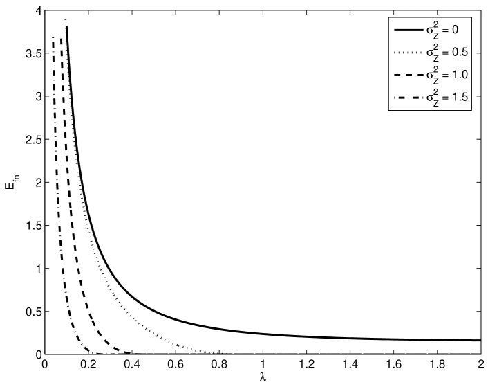
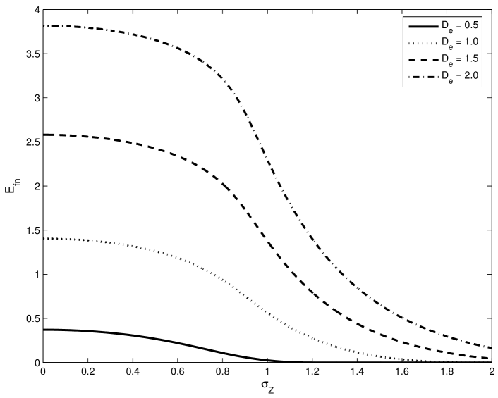
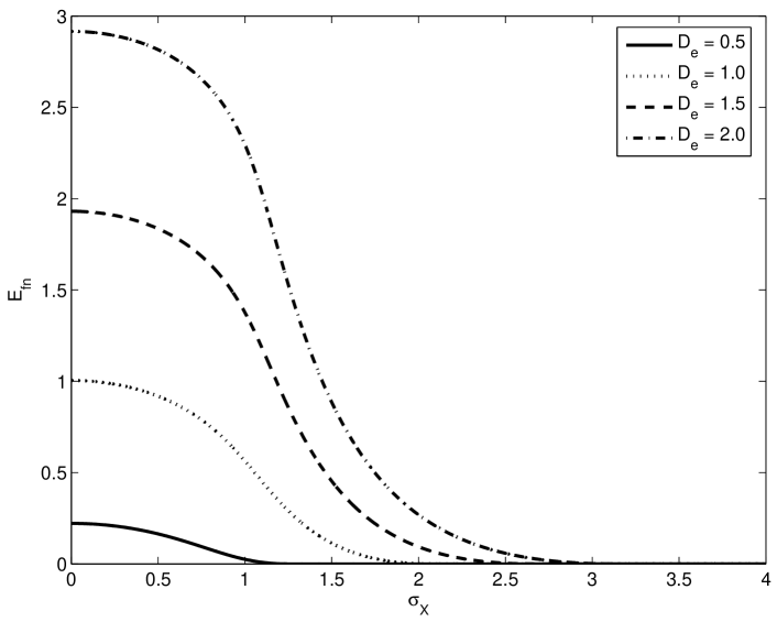
In Figs. 2, 3 and 4 the behavior of $E_{fn}^{*}$ is depicted as a function of various parameters. As expected, the false–negative exponent decreases when the false–positive exponent $\lambda$, the attack variance $\sigma_{Z}^{2}$, or the host variance $\sigma_{X}^{2}$, increase, while it increases with $D$.

Figure 2: False negative error exponent as a function of $\lambda$, for several powers of AWGN. $\sigma_{X}^{2}=1$ and $D=2$.

Figure 3: False negative error exponent as a function of $\sigma_{Z}$, for several embedding distortions. $\sigma_{X}^{2}=1$ and $\lambda=0.1$.

Figure 4: False negative error exponent as a function of $\sigma_{X}$, for several embedding distortions. $\sigma_{Z}^{2}=1$ and $\lambda=0.1$.

V-C Numerical Results

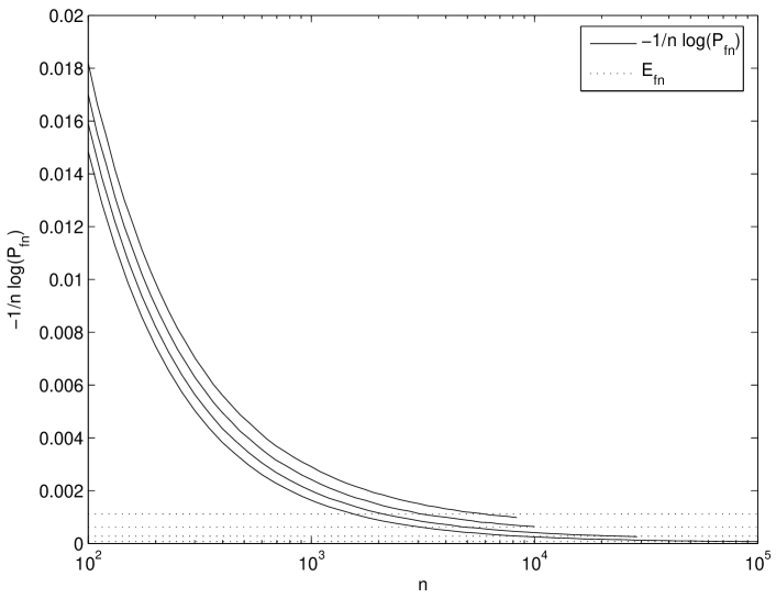
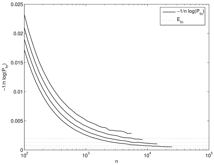
In order to validate the theoretical results with numerical ones, we compare the false–negative exponent with the empirical values of $-\frac{1}{n}\ln P_{fn}$, for large $n$. Although large values of $n$ and $-\frac{1}{n}\log(P_{fn})$ can not be considered simultaneously, due to the resulting very small probability of false negative, in Fig. 5 we can see the similarity between $E_{fn}^{*}$ and its empirical approximation when $n$ increases, for different values of $\sigma_{Z}^{2}$. Furthermore, in Fig. 6 we compare the empirical approximation of the false–negative exponent to its theoretical value for the attack–free case (special attention will be paid to this particular case in Section VI), for different values of $\lambda$. As expected, the larger is $\lambda$, the smaller is the false–negative exponent.

Figure 5: Theoretical false negative error exponent and $-\frac{1}{n}\log(P_{fn})$ as a function of the number of dimensions $n$. $D=2$, $\sigma_{X}^{2}=1$ and $\lambda=0.6$, and $\sigma_{Z}^{2}$ equal to $0.52$, $0.53$, $0.54$ and $0.55$, respectively (from top to bottom).

Figure 6: Theoretical false negative error exponent and $-\frac{1}{n}\log(P_{fn})$ as a function of the number of dimensions $n$. $D=0.75$, $\sigma_{X}^{2}=1$ and $\sigma_{Z}^{2}=0$, and $\lambda$ equal to $0.58$, $0.6$, $0.62$ and $0.64$, respectively (from top to bottom).

VI The Attack–Free Case

As a special case of Theorem 1 and Theorem 2, we calculate the false–negative exponent for the noiseless case ($\sigma^{2}_{Z}=0$). By computing the limit of $\sigma_{Z}^{2}\to 0$ in (23), it is easy to see that in the attack–free case, we have:

$$\lim_{\sigma_{Z}^{2}\rightarrow 0}r^{*} = \frac{-2D\sigma_{X}^{2}\sin^{2}\beta}{-2\sigma_{X}^{2}\cos^{2}\beta\sin^{2}\beta}=\frac{D}{\cos^{2}\beta}=\frac{D}{1-e^{-2\lambda}}.$$ (26)

To compute $\lim_{\sigma_{Z}^{2}\rightarrow 0}\frac{q^{*}}{\sigma_{Z}^{2}}$ from (24) we can use L’Hôpital’s rule. Given that

$$\lim_{\sigma_{Z}^{2}\rightarrow 0} \frac{\partial}{\partial\sigma_{Z}^{2}}\Bigg{[}\bigg{(}2D\sigma_{Z}^{2}+\sqrt{16\sigma_{Z}^{4}\sigma_{X}^{4}\cos^{4}\beta+D^{2}\left[2\sigma_{Z}^{2}-\sigma_{X}^{2}(1-\cos(2\beta))\right]^{2}}\bigg{)}\tan^{2}\beta$$

$$-2\sigma_{X}^{2}\sin^{2}\beta\left(2\sigma_{Z}^{2}+D\tan^{2}\beta\right)\Bigg{]}=-4\sigma_{X}^{2}\sin^{2}\beta,$$

and

$$\lim_{\sigma_{Z}^{2}\rightarrow 0} \frac{\partial}{\partial\sigma_{Z}^{2}}\sigma_{Z}^{2}\left[4\left(\sigma_{Z}^{2}-\sigma_{X}^{2}\sin^{2}\beta\right)\right]=-4\sigma_{X}^{2}\sin^{2}\beta,$$

we conclude that

$$\lim_{\sigma_{Z}^{2}\rightarrow 0}\frac{q^{*}}{\sigma_{Z}^{2}} = 1.$$ (27)

From (26) and (27), it is straightforward to see that the value of the false–negative exponent for the attack–free case is given by

$$\lim_{\sigma_{Z}^{2}\rightarrow 0}E_{fn}^{*} = \left\{\begin{array}[]{ll}0,&\textrm{ if }\frac{D}{1-e^{-2\lambda}}\leq\sigma_{X}^{2}\\ \frac{1}{2}\left[\frac{D}{\sigma_{X}^{2}\left(1-e^{-2\lambda}\right)}-\ln\left(\frac{D}{\sigma_{X}^{2}\left(1-e^{-2\lambda}\right)}\right)-1\right]&\textrm{ elsewhere}\end{array}\right..$$ (30)

In view of (30), it is interesting to note that as long as $D>\sigma_{X}^{2}$, $E_{fn}^{*}>0$ for any $\lambda$. In fact, under these conditions, the asymptotic value of $E_{fn}$ when $\lambda\to\infty$ is

$$\frac{1}{2}\left[\frac{D}{\sigma_{X}^{2}}-\ln{\left(\frac{D}{\sigma_{X}^{2}}\right)-1}\right],$$ (31)

coinciding with the result of [2. Corollary 1].

On the other hand, when $D\leq\sigma_{X}^{2}$ another interesting point which reflects the goodness of the proposed strategy is the computation of the range of values of $\lambda$ where $E_{fn}>0$ can be achieved. In this case, the condition to be verified is

$$\frac{D}{1-e^{-2\lambda}}>\sigma_{X}^{2},$$ (32)

implying that

$$\lambda<-\frac{1}{2}\ln\left(1-\frac{D}{\sigma_{X}^{2}}\right)=\lambda_{1},\textrm{ for }D\leq\sigma_{X}^{2},$$ (33)

whereas for the sign embedder [15], the values of $\lambda$ for which $E_{fn}>0$ are those such that

$$\frac{D}{\sigma_{X}^{2}}>\frac{1-e^{-2\lambda}}{e^{-2\lambda}},$$ (34)

or, equivalently,

$$\lambda<-\frac{1}{2}\ln\left(\frac{\sigma_{X}^{2}}{D+\sigma_{X}^{2}}\right)=\lambda_{2},\textrm{ for all }D.$$ (35)

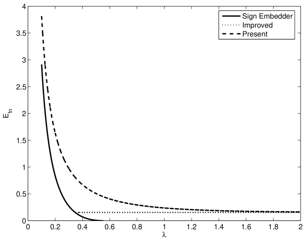
Given that $\lambda_{1}>\lambda_{2}$, larger values of false positive error exponents are allowed (while still keeping $E_{fn}>0$) by the new embedding rule. In Figure 7 we compare the bounds on the false–negative exponent for the attack–free case found in [15], with its optimal value derived here. As can be seen, the improvement owing to the optimum embedding strategy is significant, especially for small $\lambda$.

Figure 7: Comparison of the errors exponents obtained by the sign embedder described by Merhav and Sabbag [15], its improved version, and the technique presented in this work. $\sigma_{X}^{2}=1$ and $D=2$.

VII Conclusions

We derived a Neyman–Pearson asymptotically optimum one–bit watermarking scheme in the Gaussian setting, when the detector is limited to base its decisions on second order empirical statistics only. The scenario we considered is universal in the sense that the variance of both the host signal and the attack are not known to the embedder and to the detector. Our main results are simple closed–form formulas for both the optimum embedding function and the corresponding error exponents. The noiseless scenario can be seen as a special case, where we can compare the false–negative exponent achieved by the optimum scheme with the bounds derived in [15]. Interestingly, the optimum embedder is very simple thus opening the door to practical implementations.

This work can be extended in many interesting directions, including non-Gaussian settings, more complicated attacks, like de-synchronization attacks [21, 22], more detailed empirical statistics gathred by the detector, and the introduction of security considerations in the picture [23].

References

- [1] S. I. Gel’fand and M. S. Pinsker, “Coding for channel with random parameters,” Problems of Information and Control, vol. 9, no. 1, pp. 19–31, 1980.
- [2] M. H. M. Costa, “Writing on dirty paper,” IEEE Transactions on Information Theory, vol. 29, no. 3, pp. 439–441, May 1983.
- [3] I. J. Cox, M. L. Miller, and A. L. McKellips, “Watermarking as communications with side information,” Proceedings of the IEEE, vol. 87, no. 7, pp. 1127–1141, July 1999.
- [4] B. Chen and G. W. Wornell, “Quantization index modulation: A class of provably good methods for digital watermarking and information embedding,” IEEE Transactions on Information Theory, vol. 47, no. 4, pp. 1423–1443, May 2001.
- [5] M. Ramkumar and A. N. Akansu, “Signaling methods for multimedia steganography,” IEEE Transactions on Signal Processing, vol. 52, no. 4, pp. 1100–1111, April 2004.
- [6] A. Abrardo and M. Barni, “Informed watermarking by means of orthogonal and quasi-orthogonal dirty paper coding,” IEEE Transactions on Signal Processing, vol. 53, no. 2, pp. 824–833, February 2005.
- [7] F. Pérez-González, C. Mosquera, M. Barni, and A. Abrardo, “Rational dither modulation: a high-rate data-hiding method invariant to gain attack,” IEEE Transactions on Signal Processing, vol. 53, no. 10, pp. 3960–3975, October 2005.
- [8] J. R. Hernández, M. Amado, and F. Pérez-González, “DCT-domain watermarking techniques for still images: detector performance analysis and a new structure,” IEEE Transactions on Image Processing, vol. 9, no. 1, pp. 55–68, January 2000.
- [9] M. Barni, F. Bartolini, A. De Rosa, and A. Piva, “A new decoder for the optimum recovery of non-additive watermarks,” IEEE Transactions on Image Processing, vol. 10, no. 5, pp. 755–766, May 2001.
- [10] X. Huang and B. Zhang, “Statistically robust detection of multiplicative spread-spectrum watermarks,” IEEE Transactions on Information Forensics and Security, vol. 2, no. 1, pp. 1–13, March 2007.
- [11] M. Noorkami and R. M. Mersereau, “A framework for robust watermarking of H.264-encoded video with controllable detection performance,” IEEE Transactions on Information Forensics and Security, vol. 2, no. 1, pp. 14–23, March 2007.
- [12] W. Liu, L. Dong, and W. Zeng, “Optimum detection for spread-spectrum watermarking that employs self-masking,” IEEE Transactions on Information Forensics and Security, vol. 2, no. 4, pp. 645–654, December 2007.
- [13] M. L. Miller, I. J. Cox, and J. A. Bloom, “Informed embedding: Exploiting image and detector information during watermark insertion,” in IEEE International Conference on Image Processing (ICIP), vol. 3, Vancouver, BC, Canada, September 2000, pp. 1–4.
- [14] T. Liu and P. Moulin, “Error exponents for one-bit watermarking,” in IEEE International Conference on Acoustics, Speech, and Signal Processing (ICASSP), vol. 3, Hong Kong, April 2003, pp. 65–68.
- [15] N. Merhav and E. Sabbag, “Optimal watermark embedding and detection strategies under limited detection resources,” IEEE Transactions on Information Theory, vol. 54, no. 1, pp. 255–274, January 2008.
- [16] T. Furon, “A constructive and unifying framework for zero-bit watermarking,” IEEE Transactions on Information Forensics and Security, vol. 2, no. 2, pp. 149–163, June 2007.
- [17] H. V. Poor, An Introduction to Signal Detection and Estimation, 2nd ed. Springer Texts in Electrical Engineering, 1994.
- [18] T. Furon, B. Macq, N. Hurley, and G. Silvestre, “JANIS: Just Another N-order side-Informed watermarking Scheme,” in IEEE International Conference on Image Processing, vol. 2, Rochester, NY, USA, September 2002, pp. 153–156.
- [19] F. Pérez-González, F. Balado, and J. R. Hernández, “Performance analysis of existing and new methods for data hiding with known-host information in additive channels,” IEEE Transactions on Signal Processing, vol. 51, no. 4, pp. 960–980, April 2003.
- [20] R. Wong, Asymptotic Approximations of Integrals. SIAM, 2001.
- [21] M. Barni, “Effectiveness of exhaustive search and template matching against watermark desynchronization,” IEEE Signal Processing Letters, vol. 12, no. 2, pp. 158–161, February 2005.
- [22] A. D’Angelo, M. Barni, and N. Merhav, “Expanding the class of watermark desynchronization attacks,” in Proceedings of 9-th ACM Multimedia Security Workshop, Dallas, Texas, 20-21 September 2007.
- [23] M. Barni, F. Bartolini, and T. Furon, “A general framework for robust watermarking security,” Signal Processing, vol. 83, no. 10, pp. 2069–2084, October 2003.