The Complex Structure of the Cl 1604 Supercluster at $z\sim 0.9$

Abstract

The Cl1604 supercluster at $z=0.9$ is one of a small handful of such structures discovered in the high redshift universe, and is the first target observed as part of the Observations of Redshift Evolution in Large Scale Environments (ORELSE) Survey. To date, Cl1604 is the largest structure mapped at $z\sim 1$, with the most constituent clusters and the largest number of spectroscopically confirmed member galaxies. In this paper we present the results of a spectroscopic campaign to create a three-dimensional map of Cl1604 and to understand the contamination by fore- and background large scale structures. Combining new Deep Imaging Multi-object Spectrograph observations with previous data yields high-quality redshifts for 1,138 extragalactic objects in a $\sim 0.08~{}$deg² region, 413 of which are supercluster members. We examine the complex three dimensional structure of Cl1604, providing velocity dispersions for eight of the member clusters and groups. Our extensive spectroscopic dataset is used to examine potential biases in cluster velocity dispersion measurements in the presence of overlapping structures and filaments. We also discuss other structures found along the line-of-sight, including a filament at $z=0.6$ and two serendipitously discovered groups at $z\sim 1.2$.

1 Introduction

Superclusters are complex structures, consisting of multiple galaxy clusters and groups connected by chains of galaxies. They can reach sizes of $\sim 100~{}h^{-1}_{70}$ Mpc, making them the largest structures in the universe. As such, they can be used to provide an estimate of the baryonic mass fraction $\Omega_{b}$. Their frequency and topology may be used to test the veracity of large scale cosmological simulations. Because they contain structures spanning a wide range of projected and local densities, superclusters are ideal sites for studying the variety of physical processes affecting galaxy evolution, including ram pressure stripping, mergers, tidal encounters, harassment, etc. They are also sites of cluster-cluster interactions, allowing us to probe how cluster-scale interactions effect their constituent galaxies, and to probe possible differences between the dark and baryonic matter distributions.

Recent deep, wide-field imaging campaigns have begun to reveal an increasing number of superclusters at $z>0.7$. These include a $z=0.9$ compact supercluster found in the Red-sequence Cluster Survey (Gilbank et al., 2008), a structure at $z=0.89$ in the UK Infrared Deep Sky Survey (UKIDSS) Deep eXtragalactic Survey (Swinbank et al., 2007), and a large galaxy density enhancement at $z\sim 0.74$ in the COSMOS field (Scoville et al., 2007). To increase the number of well-studied high-redshift structures, we have begun the Observations of Redshift Evolution in Large Scale Environments (ORELSE) survey, a systematic photometric and spectroscopic search for structure on scales $>10$ Mpc around 20 known clusters at $z>0.6$ (Lubin et al., 2008, hereafter ORELSE I) . The Cl 1604 supercluster at $z\sim 0.9$ was the first supercluster detected as part of this survey and remains the most heavily studied structure at these redshifts. It was initially discovered as two separate clusters in the plate-based survey of Gunn, Hoessel, & Oke (1986), with redshifts and preliminary velocity dispersions measured by Postman, Lubin, & Oke (1998, 2001, hereafter P98 and P01). Deeper CCD imaging (Lubin et al., 2000) revealed a total of four distinct galaxy density peaks in a contiguous area of $10.4^{\prime}\times 18.2^{\prime}$. A large spectrographic survey using the Low-Resolution Imaging Spectrograph (LRIS; Oke et al., 1995) and the Deep Imaging Multi-object Spectrograph (DEIMOS; Faber et al., 2003) on the Keck 10-m telescopes confirmed the new cluster candidates and provided improved velocity dispersions for all four supercluster components using 230 galaxies (Gal & Lubin, 2004). The large radial depth of the supercluster ($\sim 93~{}h^{-1}_{70}$ Mpc) in comparison to the small imaging area ($4.8\times 8.5~{}h^{-1}_{70}$ Mpc) spurred a wide field imaging campaign using the Large Format Camera (LFC; Simcoe, Metzger, Small, & Araya, 2000) on the Palomar 5-m telescope. Four additional red ($1.0<=r^{\prime}-i^{\prime}<=1.4$) galaxy overdensities, identified as candidate clusters, were detected in the larger area, bringing to eight the total number of possible clusters in this structure (Gal et al., 2005).

Additional multi-object spectroscopy was undertaken to confirm the new cluster candidates and improve our understanding of the supercluster structure. In this paper we utilize our complete spectroscopic data set, with $\sim 1100$ extragalactic redshifts, to examine the three dimensional structure of the Cl1604 supercluster, improve our cluster detection algorithm, and study the cluster galaxy populations. A total of 427 galaxies have been spectroscopically confirmed within the structure, nearly doubling the number of known members. The only comparable structures at similar redshift are the $z=0.89$ UKIDSS supercluster with five density peaks (Swinbank et al., 2007) and the $z=0.9$ three-cluster system described in Gilbank et al. (2008). These two systems each have only $\sim 50$ spectroscopic members. We show that even with hundreds of members spread over the supercluster, it remains difficult to obtain consistent velocity dispersions due to the presence of overlapping structures, filaments, and changes in galaxy populations between clusters.

Section 2 describes the photometric data, density mapping and cluster detection, all of which are improvements on our earlier work. The spectroscopic data is described in §3. Cluster velocity dispersions and the associated measurement complications, along with the overall structure of the supercluster, are discussed in §4. We utilize our extensive spectroscopic sample to study photometric selection of cluster members using only three filters ($r^{\prime},i^{\prime},z^{\prime}$), and the cluster properties. Section 5 details the various fore- and background structures, including two serendipitously discovered structures at $z>1.1$ and an apparent wall at $z\sim 0.6$. A brief discussion of implications for optical surveys of high-redshift galaxy clusters and spectroscopic studies of cluster galaxy populations, is presented in §6. Throughout the paper we use a cosmology with $H_{0}=70$ km s^-1 Mpc^-1, $\Omega_{m}=0.3$ and $\Omega_{\Lambda}=0.7$.

2 Imaging and Cluster Detection

The imaging data are presented in Lubin et al. (2000) and Gal et al. (2005). We provide a brief review, along with a description of improvements to the photometric calibration and modifications made to the final density map since those publications. We have also implemented a technique to estimate the contamination of our cluster catalog by false detections, described in §2.4.

2.1 Photometric Data

The photometric data are a combination of two pointings taken in Cousins $R$ and Gunn $i$ with the Carnegie Observatories Spectroscopic Multislit and Imaging Camera (COSMIC; Kells et al., 1998) and two pointings in Sloan $r^{\prime}$,$i^{\prime}$ and $z^{\prime}$ with the LFC, both on the Palomar 5-m telescope. The layout of the imaging fields is shown in Figure 1 of Gal et al. (2005), who also describe the LFC observations and data reduction. The details of the COSMIC observations and data reduction are described in Lubin et al. (2000).

Since the publication of Gal et al. (2005), the Sloan Digital Sky Survey (SDSS; York et al., 2000) has released data in the fields covered by these pointings. We have used this data to improve the transformation of the COSMIC $R$ and $i$ magnitudes to the SDSS system and to calibrate the LFC fields. The SDSS DR5 (Adelman-McCarthy et al., 2008) was queried for the $r^{\prime}$, $i^{\prime}$ and $z^{\prime}$ model magnitudes in the region covered by our imaging. Objects were cross-identified between the SDSS catalog and our four separate pointings (two COSMIC and two LFC). The scatter between our coordinates and those of SDSS were $\sim 0.25^{\prime\prime}$ in both right ascension and declination, commensurate with the expected astrometric errors. Transformations from our photometry to SDSS were derived independently for each filter and pointing. The COSMIC $R$ and $i$ magnitudes were converted to the SDSS system using equations of the form

$$r^{\prime}_{SDSS}=A\times R+B\times(R-i)+C$$ (1)

For objects detected in only one band, we assumed $R-i=0.71$, the median color of sources in the COSMIC catalog. Similarly, the LFC data are recalibrated using

$$r^{\prime}_{SDSS}=A\times r^{\prime}_{LFC}+B\times(r^{\prime}_{LFC}-i^{\prime}_{LFC})+C$$ (2)

The depths of the LFC images are such that any object with normal colors will be detected in all three bands, unless it as the field edges or near a saturated star. We therefore apply no color terms to single-band detections. There is significant overlap between the two LFC pointings, and especially the COSMIC and LFC pointings. In our previous work, we simply trimmed the catalogs to non-overlapping areas based on visually selected coordinate limits. Here, we have improved the catalog combination by selecting objects based on photometric errors. First, the two LFC pointings were compared to each other. For sources appearing in both pointings, we use the detection with the lowest average photometric error in the three filters to create a master LFC catalog. The same procedure is applied to the two COSMIC catalogs to generate a single COSMIC catalog. These two catalogs are then compared on the basis of the $r^{\prime}$ and $i^{\prime}$ errors, with objects selected from LFC if the average photometric error $(err_{r^{\prime}}+err_{i^{\prime}})/2$ from LFC is less than that from COSMIC plus 0.05 mag. This scheme gives preference to data from the LFC because it covers a larger area and includes photometry in $z^{\prime}$. For sources where COSMIC $r^{\prime}$ and $i^{\prime}$ photometry is chosen, we incorporate $z^{\prime}$ data if it is available from LFC, or from SDSS if there is no LFC $z^{\prime}$ data or the LFC $z^{\prime}$ detection is flagged as bad. The final hybrid catalog is corrected for Galactic reddening using the dust maps from Schlegel et al. (1998) on an object-by-object basis. The $5\sigma$ limiting magnitudes are 25.2, 24.8, and 23.3 in $r^{\prime}$, $i^{\prime}$ and $z^{\prime}$, respectively.

2.2 Producing the Density Map

Following Gal & Lubin (2004), we produce a galaxy density map by adaptively smoothing a color-selected subset of galaxies in the Cl1604 field. With the additional spectroscopy presented in Gal et al. (2005) and the improved photometric calibration discussed above, some modifications to the density mapping algorithm were made. First, we used the observed colors of $\sim 300$ confirmed members to choose intervals in both the $r^{\prime}-i^{\prime}$ and $i^{\prime}-z^{\prime}$ colors that provided large numbers of supercluster galaxies and enhanced contrast relative to fore- and background structures. The limiting colors and magnitudes used were $1.0\leq(r^{\prime}-i^{\prime})\leq 1.4$, $0.6\leq(i^{\prime}-z^{\prime})\leq 1.0$ and $20.5\leq i^{\prime}\leq 23.5$. These color cuts are delineated by the black rectangles in the color-magnitude and color-color diagrams in Figure 1.

We also examined the possibility of applying color cuts based on stellar population synthesis models. Synthetic galaxy spectra were generated following the prescription used by the Red-sequence Cluster Survey (RCS, Gladders & Yee, 2005), with a Bruzual & Charlot (2003) model parameterized as a 0.1 Gyr burst ending at $z=2.5$ followed by a $\tau=0.1$ Gyr exponential decline. This model predicts colors of $(r^{\prime}-i^{\prime})=1.05$ and $(i^{\prime}-z^{\prime})=0.78$ at $z=0.9$; they are plotted as the yellow bars and crosses in Figure 1. The observed $(r^{\prime}-i^{\prime})$ colors are about 0.2mag redder. Although the BC03 model colors are within our broad color cuts, the empirical colors, by construction, provide optimal detection of structure at the redshift of interest. Tests of other models for the red galaxy population, including single starbursts with either instantaneous or exponentially declining bursts, showed that expected galaxy colors varied a few tenths of a magnitude between models. Therefore, we use our empirically confirmed color cuts to produce a final density map. As discussed in ORELSE I, the star formation history chosen by the RCS yields model colors that, while within our broad color cuts, do not match perfectly the observed red sequences in any of our structures at $0.7<z<1.1$. This is unsurprising as the average galaxy’s star formation history varies with environment, and there remain unresolved issues with stellar population synthesis models. As models improve and large surveys like ORELSE, RCS and PISCES (Panoramic Imaging and Spectroscopy of Cluster Evolution with Subaru, Kodama et al., 2005) obtain spectroscopy and map out the observed red sequence colors as a function of redshift, it will be possible to find BC models that better fit the data.

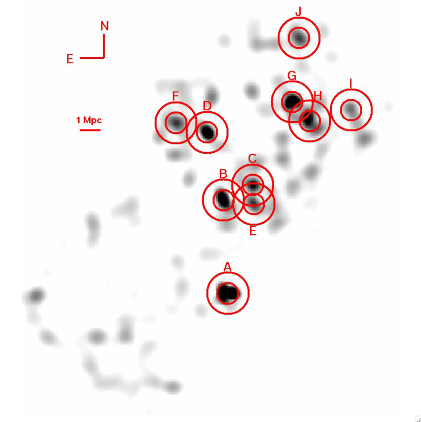
Figure 2: Adaptive kernel density map of color-selected galaxies in the Cl1604 region. Detected cluster and group candidates are marked with red circles of $0.5h^{-1}_{70}$ and $1.0h^{-1}_{70}$ radius, and labeled with an identifying letter.

The color and magnitude cuts select only 722 objects out of an initial catalog of $\sim 12,000$ with $i^{\prime}<23.5$. An adaptive kernel smoothing is applied using an initial window of $0.75h^{-1}_{70}$ Mpc and 10 arcsecond pixels. We use a smaller kernel than the $1h^{-1}_{70}$ Mpc radius applied in Gal & Lubin (2004) because our extensive spectroscopy showed that small groups were being blended into single detections in the density map. The smaller kernel also enhances the contrast of small groups against the background, making detection of such low-mass systems easier. The new density maps are shown in Fig. 2, with the detected overdensities marked. Comparison to Figure 1 of Gal & Lubin (2004) shows that similar structures are found with the new color cuts.

2.3 Cluster Detection

The density maps are used primarily to provide a visual locator for intermediate density large scale structure in the imaging field. Filaments and cluster infall regions can cover significant portions of the observed area, but at relatively low contrast, making it difficult to detect them and define their boundaries. Identification of such overdense regions is used primarily to direct placement of follow-up observations, especially slitmasks for multi-object spectroscopy. However, it is necessary to provide a consistent detection mechanism for finding clusters and groups in the ORELSE survey fields, described below.

Cluster detection is performed by running SExtractor (Bertin & Arnouts, 1996) on the adaptively smoothed red galaxy density map. In Gal & Lubin (2004) we relied on visual inspection of the density map and comparison to the poorest (lowest velocity dispersion) cluster in the field, Cl1604+4316 (cluster C). With the addition of the spectroscopy presented in Gal et al. (2005) and herein, the projected overdensities can be better characterized, and detection parameters tuned to detect real structures. We tested various combinations of detection threshold and minimum area, all taken from Cluster C. This cluster still has the lowest reliably measured velocity dispersion, as detailed in §4. SExtractor was run with these parameters, and the resulting detections compared to our spectroscopic cluster catalog to ensure that all confirmed clusters and groups were detected. We also examined the false detection rate, described in the following section. The final set of detection parameters has high detection efficiency (100% by design) for the confirmed structures while yielding less than one false detection on average in the survey area.

A total of 10 cluster and group candidates are detected, similar to those found in Gal & Lubin (2004). Where possible, we use the same naming and lettering convention as our previous work to refer to specific clusters. Table 1 provides the details of each cluster. Column 1 lists the single letter denoting each cluster (following the nomenclature of Gal et al., 2005), while Column 2 provides the full name. Columns 3 and 4 give the updated cluster coordinates. The remaining columns provide information on membership, redshifts, and velocity dispersions, as detailed in §4.

2.4 Cluster Detection Thresholds

Because one of our goals is the detection of low-mass group-like structures in the Cl1604 field, our detection thresholds are generous in the sense that we may suffer from a high false detection rate, even with the stringent color cuts. Our method for setting thresholds and estimating contamination rates is detailed in ORELSE I; however we outline it briefly here since the Cl1604 data have been used to tune the parameters.

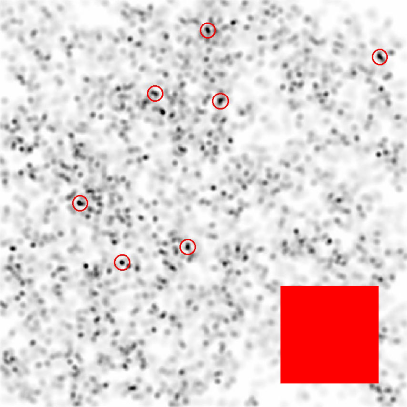
Figure 3: Adaptive kernel density map of a Raleigh-Levy simulated galaxy distribution covering $2.2^{\circ}$ on a side. Cluster candidates, which would be false detections since there are no real structures in this map, are marked with circles of $1.0h^{-1}_{70}$ radius (for $z=0.9$). The shaded box in the bottom right covers an area equal to that imaged for Cl1604.

We use the NOAO Deep Wide Field Survey (Jannuzi & Dey, 1999) to study possible contamination by ’field’ galaxies having colors meeting our selection criteria. We cannot rely on our imaging survey because it is entirely targeted at known high-density regions of the universe. Thus, we use the NOAO DWFS to derive the statistical properties of the red galaxy distribution. The third data release (DR3) in the Bootes field covers an area of nine square degrees, in the B_W, R and I filters. In brief, we transform the DWFS $R$ and $I$ data to the SDSS $r^{\prime}$ and $i^{\prime}$ systems, and apply our $r^{\prime}-i^{\prime}$ color cut and $i^{\prime}$ magnitude limit. Because there is no $z^{\prime}$ photometry in the DWFS, we then assume that field galaxies meeting only the $r^{\prime}-i^{\prime}$ cut (numbering $N_{1color,DWFS}$) have a similar projected distribution as those that also meet our $i^{\prime}-z^{\prime}$ cuts, only with a higher space density. We tested this assumption by examining the galaxy distributions far from cluster centers in density maps using our own data, applying only the $r^{\prime}-i^{\prime}$ cut and cuts in both colors. We find no significant differences. Following Postman et al. (1996) and Gal & Lubin (2004), we use the color- and magnitude-selected subset of the DWFS data to compute Raleigh-Levy (RL) parameters for galaxies meeting our color cuts, which we then use to generate simulated galaxy distributions. These are then used to produce density maps on which we run SExtractor. The SExtractor parameters DETECT_THRESH and MIN_AREA ($\pi\times r_{test}^{2}$) are varied, using values of the galaxy density at different radii $r_{test}$ from the center of cluster C in Cl1604, until a set of values is found that successfully detects the confirmed clusters in Cl1604 while yielding low contamination. We find that an area of 47 pix², corresponding to a radius of 0.3$h^{-1}$ Mpc, allows us to detect all of the spectroscopically confirmed cluster candidates in the real data, while minimizing the number of detections in the RL simulations, which should all be chance projections. The median number of false detections expected in the area imaged for Cl1604 is $N_{false}=1.4$, compared to the ten candidates detected. Figure 3 shows an example RL simulated map $2.2^{\circ}$ on a side, with the eight ’false’ candidates detected using our optimal SExtractor parameters marked. The shaded box in the bottom right covers an area equal to that imaged for Cl1604.

3 Spectroscopic Data

The spectroscopic observations consist of five separate datasets:

1. Spectra taken using LRIS as part of the original Oke, Postman, & Lubin (1998) survey.

2. Additional LRIS spectra taken in May 2000, covering the area imaged with COSMIC.

3. DEIMOS spectra covering the same area taken in 2003.

4. DEIMOS spectra taken in 2005 and 2006, using color selection and spanning a larger area imaged with LFC.

5. DEIMOS spectra covering the same area as before, but including X-ray, radio, HST ACS and new color-selected sources.

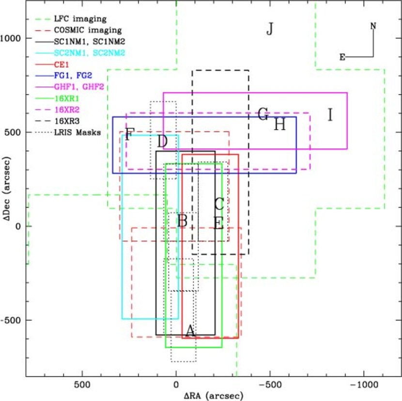
Figure 4: Layout of spectroscopic observations in the Cl1604 field. The regions imaged from the ground with COSMIC (red dashed lines) and LFC (green dashed lines) are shown, along with the LRIS masks observed in May 2000 as dotted lines. The eleven DEIMOS masks from the three campaigns discussed in the text are also plotted, along with the locations of the clusters detected from the density map.

Each sample is described in more detail below, with the layout of all masks shown in Fig. 4.

3.1 LRIS and DEIMOS Observations

The original observations of Cl1604+4304 and Cl1604+4321 (clusters A and D) were taken in the late 1990s with LRIS on the Keck I and II telescopes and are detailed in Oke, Postman, & Lubin (1998), Postman, Lubin, & Oke (1998) and Lubin et al. (1998). These initial slitmasks targeted all galaxies with $R<23.5$ based on earlier imaging with LRIS. It is important to note that no color selection was utilized in selecting galaxies to observe; therefore, blue galaxies at the supercluster redshift are more likely to be observed compared to the DEIMOS data discussed below. Redshifts were measured for 103 and 135 galaxies in the fields of Cl1604+4304 and Cl 1604+4321, respectively. Imaging of a larger region with COSMIC on the Palomar 200-inch telescope was used to design additional LRIS slitmasks, targeting an area including clusters B and C. Objects with magnitudes down to $i=23.0$ were included, with priority given to red galaxies. Six additional LRIS masks with 156 targets were observed in May 2000. Median velocity errors for the LRIS data are 150 km s^-1.

Starting in May 2003, Cl1604 was observed with DEIMOS on the Keck II telescope. We briefly describe these observations here; the details will be provided in a future paper releasing multi-wavelength data, including redshifts, in the Cl1604 field. The first DEIMOS observations also spanned the region imaged with COSMIC, and are detailed in Gal & Lubin (2004). Galaxies as faint as $i\sim 24$ were observed, with higher priority for red galaxies based on COSMIC $R-i$; only 60% of the targeted objects met the red galaxy color cut. We used the 1200 l/mm grating, blazed at 7500Å, and $1^{\prime\prime}$ slits, resulting in a pixel scale of 0.33Å pix^-1, a resolution of $\sim$1.7Å (68 km s^-1), and typical spectral coverage from 6385Å to 9015Å. Data were reduced using the DEEP2 version of the spec2d and spec1d data reduction pipelines (Davis et al., 2003). Since the publication of Gal & Lubin (2004), the DEEP2 team has made available their redshift measurement pipeline zspec (Cooper et al., 2007) and all DEIMOS redshifts have now been obtained using this package. Typical redshift errors using this method are 25 km s^-1, nearly a factor of four improvement over our original measures.

Using the multiband LFC photometry from Gal et al. (2005), galaxies with $20.5\leq i^{\prime}\leq 24.0$ were targeted over a larger area based on both color and magnitude. Five DEIMOS masks, labeled CE1, FG1, FG2 and GHF1 and GHF2 in Fig. 4 were observed in 2005 and 2006 using these ground-based color selection criteria. The Cl 1604 supercluster was also the subject of a two-band 17-pointing mosaic with the Advanced Camera For Surveys (ACS), a two-pointing ACIS-I observation with Chandra (Kocevski et al., 2008), and a Very Large Array B-Array 1.4 Ghz radio map (Miller et al., 2008). These multi-band data were used to design additional DEIMOS masks. The primary sample included X-ray and radio sources within the ACS mosaic, and red-sequence galaxies selected on the basis of the high-precision ACS colors. Secondary samples included X-ray and radio sources outside the ACS mosaic and bluer galaxies within the ACS mosaic. Lower priority samples include red galaxies outside the ACS mosaic, then bluer (by as much as 0.3^mag) galaxies outside the ACS area, and finally any galaxy not already selected by the above criteria. We observed three of these masks in June 2007.

Figure 4 shows the positions of the LRIS masks observed in May 2000 as well as all eleven DEIMOS masks. The locations of the cluster and group candidates are also marked. This figure makes evident the uneven spectroscopic coverage of the supercluster. Especially noteworthy is the extensive LRIS coverage of Clusters A and D; because no color selection was used for the original LRIS masks, the blue (presumably star-forming) populations in these clusters will be better sampled. Nevertheless, even in regions where there is only DEIMOS coverage, $\sim 50\%$ of the targeted galaxies were outside the red sequence. We explore the dependence of cluster velocity dispersions on the population sampling in §4.1.3.

In addition to the targeted objects, numerous serendipitous spectra were found by visual inspection. These objects had their extraction windows set manually, but were otherwise run through the same pipelines as the target objects. Two of us (RG and BL) systematically inspected all of the spec2d created serendip one-dimensional spectra to determine whether these extractions contained genuine serendips and to confirm their redshifts. A significant number of serendips (180 extragalactic objects, 138 with Q$>2$) were found in our DEIMOS data. Many of these at the supercluster redshift show strong [OII] emission and little continuum. These objects represent a different population than the primary targets (red sequence galaxies) and may impact the velocity dispersion determination, explored in §4.1.3.

3.2 Combined Spectroscopy Results

All of the spectroscopic data were combined into a single master catalog. For objects observed with both LRIS and DEIMOS, we used the DEIMOS results due to the improved redshift accuracy with the higher dispersion grism and typically higher signal-to-noise ratio. Serendipitous spectra were matched to photometric objects from ACS and/or Palomar imaging. In a few cases no counterpart was found, usually for single emission line spectra, some of which are likely to be Ly$\alpha$ emitters at $z>4$ (Lemaux et al., 2008a). Each photometric identification was examined visually (by RG) to check for blends, interacting galaxies and misidentifications. A set of flags was added to the catalog, identifying whether or not the object was detected and/or blended in either or both the ACS and Palomar images. The final catalog contains a total of 1,671 unique objects. Of these,

• 1,215 are extragalactic objects, of which 1,138 have Q=3 or Q=4;

• 1,148 (1,089 with Q=3 or 4) of the above are matched to a cleanly detected (not blended) photometric object in either the ACS or ground-based imaging;

• 140 are stars;

• 427 are in the redshift range of the supercluster ($0.84\leq z\leq 0.96$), of which 413 have Q=3 or Q=4;

• 417 (404 with Q=3 or 4) of the supercluster members have clean photometry.

The top panel of Figure 5 shows the redshift distribution of the Q=3 or 4 extragalactic objects (solid line), as well as for objects with Q$>2$ (dotted line). The bottom panel shows only the redshift range of the supercluster ($0.84\leq z\leq 0.96$) with redshift bins of $\Delta z=0.001$. In addition to a number of clear redshift peaks in the supercluster, many intervening structures are noticeable, discussed in detail in §5. We use only the most reliable (Q=3 or 4) redshifts for all of the analyses presented here.

4 Cluster Properties and Supercluster Structure

4.1 Individual Cluster Properties

Nine of the ten cluster candidates listed in Table 1 have been extensively mapped in our spectroscopic campaign, with only Cluster J lacking spectroscopic coverage. We use our dataset to examine the redshift distribution around each cluster candidate, both to verify the structures and measure velocity dispersions. Because of our generous detection threshold, we expect to find structures consistent with modest sized groups as well as richer clusters. In some cases, clusters overlap each other even with the smallest radius used, and almost all clusters have companions within 1 $h^{-1}_{70}$ Mpc, as seen in Fig. 2. The complex supercluster structure makes separation of individual cluster components difficult and in some cases impossible. Information on both position and velocity must be incorporated; even so, individual clusters or groups may exhibit significant substructure (Dressler & Shectman, 1988).

4.1.1 Velocity Dispersions

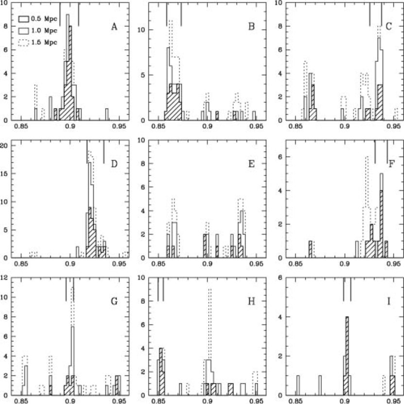
Figure 6: Redshift histograms for Clusters A-I. The shaded regions show the distribution within a projected radius of $0.5h^{-1}_{70}$ Mpc, while the solid and dashed lines correspond to radii of 1 and 1.5 $h^{-1}_{70}$ Mpc, respectively. The vertical lines at the top of each panel demarcate the final redshift range used to compute the velocity dispersion for each cluster. Note that the vertical axes have different ranges. Cluster E is not marked due to contamination from B and C.

We use the cluster centers determined by SExtractor from the density map when measuring cluster redshifts and velocity dispersions. We note that the spectroscopic coverage varies greatly from cluster to cluster, as seen in Fig. 4. We first construct redshift histograms within 0.5, 1.0 and 1.5 $h^{-1}_{70}$ Mpc projected radii centered on each cluster. These are plotted in Figure 6 for clusters A-I. The shaded region, solid line and dashed line show the redshift distributions within 0.5, 1.0 and 1.5 $h^{-1}_{70}$ Mpc, respectively. An initial redshift range (typically spanning $\sim 3000$ km s^-1) for each cluster is then selected by visual inspection of these plots, attempting to avoid clear redshift peaks from adjacent structures.

The extensive overlap between structures results in contamination of the redshift distributions. A good example is Cluster C ($z\sim 0.935$), where we see numerous galaxies at $z\sim 0.865$ within a projected $0.5h^{-1}_{70}$ Mpc radius. In this case, the redshift separation is large enough to easily distinguish the two populations. More complicated overlaps, such as between D and F, where the redshift separation is only $\Delta z\sim 0.01$, are difficult to resolve. In such cases, neglecting the overlap may lead to overestimation of the velocity dispersion. Conversely, applying strict redshift limits to avoid such overlaps can artificially lower the measured dispersion.

For each cluster we follow the procedure described in Gal et al. (2005) and Lubin et al. (2002). After the initial redshift range is chosen, the cosmologically corrected velocities relative to the median cluster redshift are calculated for each galaxy within the three radii. The initial velocity windows are typically $\pm 3000$ km s^-1, sufficiently broad to avoid biasing the dispersion estimates to lower values. These distributions are iteratively clipped at $3\sigma$, where $\sigma$ is the biweight dispersion computed by ROSTAT (Beers, Flynn, & Gebhardt, 1990). Typically from 0-2 galaxies are excluded from each cluster by this clipping. The final dispersions are computed using the biweight estimate of the scale, with errors taken from the jackknife confidence interval on the biweight scale. These have been shown to be well-behaved under most circumstances for modest sample sizes (Beers, Flynn, & Gebhardt, 1990).

Contamination from fore/background clusters, groups and filaments could bias the measured velocity dispersions and their associated errors when using ROSTAT (Andreon, 2008). We have used quite stringent spatial and redshift cuts to establish the starting ranges for velocity dispersion measurement, which reduces the contamination. We also examined the agreement between the $3\sigma$-clipped standard dispersion, the biweight estimate of the scale, and the gapped estimator, noting how many (out of 3 maximum) of these estimators agree within the quoted errors. The results are presented in Table 1. Columns 5, 8 and 11 give the number of spectroscopically confirmed members within 0.5, 1.0 and 1.5 $h^{-1}_{70}$ Mpc projected radii, respectively. These numbers include only those galaxies used to compute the velocity dispersions within each radius. Columns 6, 9 and 12 provide the median redshift for each cluster within each of the three radii, while Columns 7, 10 and 13 list the computed velocity dispersions and their errors. Columns 7, 10 and 13 also include, in parentheses, the number of different dispersion estimators that agree within the errors. Despite having fewer galaxies, we would prefer the final velocity dispersions to be those measured within 0.5 $h^{-1}_{70}$ Mpc, since the smaller radius reduces contamination from overlapping clusters. However, only Clusters A-D have sufficient members within this small radius to compute dispersions, so we quote the dispersions using the 1.0 $h^{-1}_{70}$ Mpc radius throughout. The final redshift intervals used for this radius are shown in Fig. 6 as the vertical lines near the top of each panel. The sole exception is Cluster E, which appears to be a superposition of components related to Clusters B and C. We, therefore, measure no velocity dispersion and do not show its color-magnitude diagrams.

4.1.2 Velocity Dispersions, Errors and the Effect of Interlopers

If we assume that the velocity dispersion errors quoted in Table 1 are due purely to sample size, then we would expect the errors to decrease with the square root of the number of galaxies sampled. This is almost exactly true for Clusters A and D, and the quoted dispersions using different radii all agree within $1\sigma$. For Cluster B, the three quoted dispersions agree very well, even though the estimated error remains nearly constant with sample size. For the remaining structures, which all have much sparser sampling and appear to be intrinsically poorer, the effects of small numbers and contamination from interlopers make reliable dispersion estimates impossible. A good example is Cluster G, where the estimated error increases despite the larger sample size when moving from 1.0 to 1.5 $h^{-1}_{70}$ Mpc projected radius. We see from Fig. 4 that Clusters G and H are very close to each other. Clearly, even with extensive spectroscopy it is not always possible to definitively assign membership of individual galaxies to specific clusters or groups. The behavior of our dispersions and associated errors shows that systematic errors remain an important contributor, likely due to galaxies that are not physically bound to each cluster found in the redshift range and spatial region used in the calculation. This suggests that dense sampling of cluster cores may be necessary to obtain reliable velocity dispersions. However, comparison of such data to models requires understanding of possibly cluster mass dependent biases of the observed versus true dispersions.

Another possibility, discussed by Andreon (2008), is that the dispersions and errors are not measured correctly due to interlopers from filaments. The presence of an approximately uniform background results in artificially inflated dispersions. This background contribution is important as long as it is at least a modest fraction of the total sample. In Andreon (2008) they show the exaggerated case of 500 cluster members and 500 interlopers. We utilize Clusters A and D to see if such interlopers affect significantly our dispersions.

One way to estimate the number of potential interlopers is to count galaxies within the same projected radius as the final assigned members, but in a velocity range outside the final window used for the dispersion calculation. Examination of Fig. 6 shows that there are only a few galaxies outside the final velocity windows used for Clusters A and D, but less than $\Delta v=4000$ km s^-1 away. This provides an estimate of the density of interlopers in velocity space near each cluster. As an example, consider Cluster A, using the 1.0 $h^{-1}_{70}$ Mpc radius. The final velocity window containing all members used to calculate the dispersion is a top hat with half-width $dv=1493$ km s^-1. We count all galaxies $N_{int}$ in the same 1.0 $h^{-1}_{70}$ Mpc radius, but with velocities between $-2dv...-dv$ and $dv...2dv$. If the background galaxy distribution is constant with velocity, $N_{int}$ is also the expected number of interlopers within the cluster velocity range ($-dv$ to $+dv$). For Cluster A, we find $N_{int}=(1,3,3)$ for R$=0.5,1.0,1.5h^{-1}_{70}$ Mpc radii. If these are all taken to be interlopers, they correspond to possible contamination rates of 5%, 9% and 8%, respectively. For Cluster D, we find similar results with $N_{int}=(1,2,6)$ and contamination rates of 3%, 4% and 8%. This analysis assumes that all galaxies with velocities between $-2dv...-dv$ and $dv...2dv$ are interlopers, thus providing an estimate of the maximum effect that they could have.

To see if the presence of such objects could effect the velocity dispersions, we perform a Monte Carlo simulation with Clusters A and D, using all three projected radii. We remove $N_{int}$ galaxies from the velocity range $-dv...dv$. One galaxy is removed in each velocity bin of width $2dv/N_{int}$, ensuring that the likelihood of removal is flat across the entire velocity range, corresponding to contamination by a constant background. The velocity dispersion and associated errors are recomputed using the new sample, and this procedure is repeated 1000 times for each cluster and radius combination. We compute the mean velocity dispersion (using the biweight dispersion estimator from ROSTAT) and mean error (jackknife of the biweight from ROSTAT) for each cluster and radius combination from the 1000 Monte Carlo runs. We then examine (a) the difference between these velocity dispersions and the original estimates and (b) the rms scatter within the 1000 Monte Carlo runs. We find that the velocity dispersions calculated after removing potential interlopers are only $1-5\%$ lower than the initial estimates. As an example, the original dispersions for Cluster A using the three radii are 532, 619, and 682 km s^-1. The interloper-corrected estimates are 532, 595, and 647 km s^-1, corresponding to reductions of 0%, 4.0% and 5.4%, respectively. The scatter among the Monte Carlo runs is 10-50 km s^-1, depending on the cluster and radius used. Adding this in quadrature to the already quoted error estimates would only increase the errors by $\sim 10\%$. These results demonstrate that there is little bias in our velocity dispersions due to interlopers.

4.1.3 Dependence of Velocity Dispersions on Sampling and Galaxy Colors

In addition to the possibility of interlopers, the spectroscopic sampling is significantly variable from cluster to cluster, as described in §3. This is especially true for Clusters A and D, which have extensive LRIS data where no color cuts were applied. Because the measured velocity dispersions for these (and other) clusters in Cl1604 have decreased significantly compared to our and others’ earlier observations (Gal & Lubin, 2004, P98, P01), we examine how the sampling (by instrument and by color) affects the current results.

First, for Clusters A and D, we simply excluded the LRIS redshifts and measured their velocity dispersions using only the DEIMOS data. The DEIMOS data have significantly smaller redshift errors, and using only the DEIMOS data makes the instrumental sampling similar for all of the clusters. We use the 1 $h_{70}^{-1}$ Mpc radius for this test to maintain a significant number of galaxies. Cluster A has 26 galaxies with Q$>2$ DEIMOS redshifts, yielding a velocity dispersion $\sigma=691\pm 103$ km/s, consistent with the results including LRIS (32 galaxies, $619\pm 96$ km/s). For Cluster D, the DEIMOS-only dispersion is $\sigma=445\pm 134$ km/s from 29 galaxies, compared to $\sigma=590\pm 112$ km/s from 53 galaxies when LRIS data are included. These values are also consistent within the errors, although the lowered dispersion when only DEIMOS data are used may be due to the large number of LRIS redshifts excluded. The LRIS-observed galaxies are, on average, bluer than the DEIMOS-observed ones, and may therefore have a different dispersion. We note, however, that nearly half the DEIMOS targets are also outside the red sequence. We conclude that the inclusion of LRIS data for some clusters does not significantly alter our results.

We further examined if the computed dispersion is different for red sequence galaxies than for the cluster population as a whole. Such segregation was already shown by Zabludoff & Franx (1993), who found higher dispersions for late-type galaxies than for early-types in rich, low redshift clusters. This effect should be even more pronounced at high redshift, where the clusters are less evolved. Furthermore, since there is a color-density relationship, using only the red galaxies should reduce the contribution of infalling groups/filaments at the cost of smaller sample size. We applied the same color limits used for the density mapping ($1.0\leq(r^{\prime}-i^{\prime})\leq 1.4$, $0.6\leq(i^{\prime}-z^{\prime})\leq 1.0$) and a magnitude limit of $i^{\prime}\leq 24.0$ to the spectroscopic samples in each cluster. Only Clusters A, B and D have sufficient (though still small) numbers of red galaxies for this exercise. Using the 1 $h_{70}^{-1}$ Mpc radius to maintain a significant number of galaxies, we find:

Cluster A: full sample 32 galaxies, $\sigma=619\pm 96$ km/s ; color cut 18 galaxies $\sigma=327\pm 62$ km/s
Cluster B: full sample 32 galaxies, $\sigma=811\pm 76$ km/s ; color cut 12 galaxies $\sigma=778\pm 127$ km/s
Cluster D: full sample 53 galaxies, $\sigma=590\pm 112$ km/s ; color cut 16 galaxies $\sigma=338\pm 71$ km/s

In all three cases, the red galaxies have a lower velocity dispersion. For Cluster A the difference is $3.0\sigma$, while for Cluster D it is only $2.2\sigma$, and less than $1\sigma$ for Cluster B. As shown above, these changes are not the result of instrumental coverage (DEIMOS or LRIS), so the differences must reflect the properties of the distinct galaxy populations. It is interesting to note that our Chandra observations find Cluster A to be the most X-ray luminous system in the supercluster, exhibiting a relaxed and well-established intra-cluster medium (Kocevski et al., 2008). If the system formed at an earlier epoch than Clusters B and D, it is expected that the primordial red galaxy population would have had more time to fully virialize and establish a much different dispersion than any infalling blue galaxy population. The lack of a significant difference in the velocity dispersions of blue and red galaxies in Cluster B, and to a lesser extent Cluster D, may be further evidence that the systems are undergoing collapse or possible merger processes. These results again suggest that one must exercise caution both when selecting galaxies for spectroscopic followup using colors and when interpreting the resulting cluster velocity dispersions. Our sample is extremely limited, but is one of the first to have so many cluster members at redshifts near unity. The fact that the pattern of velocity dispersion as a function of galaxy color is not the same from cluster to cluster may imply that followup of only red-sequence galaxies might yield biased or inconsistent results, especially if the red vs. blue galaxy dispersion depends on the cluster mass or formation epoch. This could also be true if only the most luminous cluster galaxies are used since they are much more likely to have red colors. Larger samples with deep spectroscopy of clusters in various evolutionary stages will be necessary to clarify these findings.

The velocity dispersions computed for Clusters A and D, using all galaxies within 0.5 or 1 $h^{-1}_{70}$ Mpc radii, are a factor of two below the initial estimates from Postman, Lubin, & Oke (1998) and Postman, Lubin, & Oke (2001). The $\sigma$ values derived here would place these clusters closer to the $L_{X}-\sigma$ relation, alleviating the X-ray under-luminosity discussed in Lubin et al. (2004). This consistency makes it tempting to assume that these are the correct dispersions to use; however, the morphological and/or color sampling is not the same from cluster to cluster (both due to sampling differences and population variations), and the X-ray luminosities may also be unreliable due to point source contamination. These results clearly require detailed comparison to simulations to see what population mix is best for producing reliable velocity dispersions that trace the gravitating halo mass. Simplistic approaches to measuring cluster dispersions, especially at an epoch when they are still accreting significant portions of their final galaxy (and mass) content, are not likely to be reliable except for the most massive evolved systems.

4.1.4 Substructure

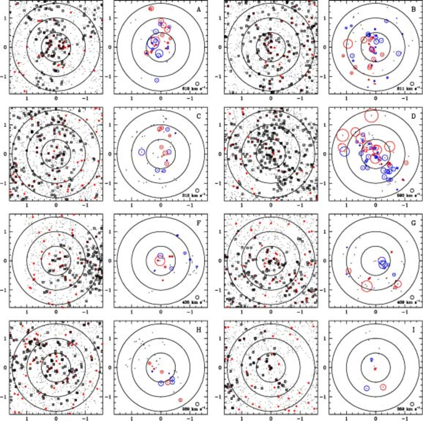
Figure 7: Spectroscopic coverage and position-velocity diagrams for 8 clusters in Cl1604. There are two panels for each cluster, each covering an area of 3.2 $h^{-1}_{70}$ Mpc on a side. The left panels show all galaxies with $20.5<i^{\prime}<24$ as small black dots, while red galaxies used to make the density map are shown as larger red dots. Black squares outline the spectroscopic targets. The right panels for each cluster plot all galaxies in the supercluster redshift range ($0.84\leq z\leq 0.96$) as small black dots. The final members of each cluster are then circled, with red circles for galaxies with higher recession velocities than the cluster mean, and blue for those galaxies with lower velocities. The circles are scaled by $v_{gal}/\sigma_{clus}$, with the scaling shown in the lower right corner of each panel. In both panels, the three large circles correspond to radii of 0.5, 1.0 and 1.5 $h^{-1}_{70}$ Mpc, used to measure velocity dispersions.

To better understand the individual cluster structures and possible contamination from neighboring clusters and filaments, we examined the spectroscopic coverage and position-velocity distributions within each cluster. These are shown in Figure 7 for all clusters except E (which has no clear redshift peak) and J (which has no spectroscopic coverage). There are two panels for each cluster, each covering an area of 3.2 $h^{-1}_{70}$ Mpc on a side. The left panels show all galaxies with $20.5<i^{\prime}<24$ as small black dots. Essentially, these are all possible spectroscopic targets in the field regardless of priority. Red galaxies used to make the density map are shown as larger red dots. The concentrations in the centers of most clusters are evident, and in later DEIMOS masks these were prioritized. Black squares outline the galaxies with spectroscopic redshifts. Spectroscopic targets which met the density map color criteria are almost always cluster members, highlighting the efficiency of our color cuts in selecting supercluster members. Clusters A and D have very dense coverage because they were the first to be discovered by Gunn, Hoessel, & Oke (1986) and were the targets of initial LRIS spectroscopy. The three large circles correspond to radii of 0.5, 1.0 and 1.5 $h^{-1}_{70}$ Mpc, used to measure velocity dispersions. The right panels for each cluster plot all galaxies in the supercluster redshift range ($0.84\leq z\leq 0.96$) as small black dots. The final members of each cluster (as determined using ROSTAT within the 1.5 $h^{-1}_{70}$ Mpc radius) are then circled. Red circles are used for galaxies with higher recession velocities than the cluster mean, while blue circles show those blueshifted relative to the cluster mean. The circle sizes are scaled by the ratio of the galaxies’ cluster-centric radial velocity to the cluster’s velocity dispersion, $v_{gal}/\sigma_{clus}$. The corresponding velocity dispersion is shown in the lower right corner of each panel, along with a circle for $v_{gal}=\sigma_{clus}$. Cluster E has no redshift limits marked and no velocity dispersions measured due to contamination from B and C.

Examination of Fig. 7 demonstrates that even the very well-sampled clusters (A, B and D), with over thirty members within a 1 $h^{-1}_{70}$ Mpc radius, show visual evidence for substructure. Cluster D in particular appears very elongated in the NE-SW direction. Cluster B shows velocity segregation, which could be interpreted as either substructure or a triaxial cluster, elongated in the radial direction and oriented at a slight angle to the line-of-sight. To quantify the amount of substructure, we performed Dressler & Shectman (1988) tests on Clusters A, B and D using the spectroscopically confirmed members within a 1.0 $h^{-1}_{70}$ Mpc radius (32, 32 and 53 galaxies, respectively). Also known as the $\Delta$ or DS test (Pinkney et al., 1996), this statistic looks for velocity substructure among galaxies near each other in projection as an indicator of merging components. The DS statistic was shown by Pinkney et al. (1996) to be the most sensitive of the five different substructure estimators they examined, and works well even for moderate samples with only $\sim 30$ velocities per cluster. This test indicates no substructure in Cluster A, consistent with its appearance in Fig. 7. Cluster B, although showing two velocity subclumps (Fig. 6), has no significant substructure based on the DS test. This may be the result of having two subclumps very well aligned along the line-of-sight, a situation to which the DS-test is not sensitive. Cluster D has the highest likelihood of substructure, with the null hypothesis (no substructure) rejected at the 93% confidence level. This is consistent with the evident elongation at an angle to the line of sight and the velocity segregation between the NE and SE parts of the cluster.

Recent work using both optical and X-ray data (Sereno et al., 2006; Paz et al., 2006; Plionis et al., 2006; De Filippis et al., 2005) has shown that many clusters and groups are quite strongly triaxial, consistent with large simulations such as those of Jing & Suto (2002). Additionally, the Cl1604 supercluster is extremely elongated along the line-of-sight, and we expect, based on Hubble volume simulations, that the clusters will be aligned with the supercluster (Lee & Evrard, 2007). Further understanding of the cluster dynamics will require detailed comparison to large $N$-body simulations as well as modeling of the Cl1604 supercluster in particular.

4.1.5 Color-magnitude diagrams

The presence of a strong color-magnitude relation (CMR), the red sequence for early-type galaxies, has long been observed (Visvanathan & Sandage, 1977; Bower et al., 1992) and used for cluster detection (Gladders & Yee, 2000). At the redshift of the Cl1604 supercluster, galaxies become too small to classify morphologically from ground-based images. Recent work has used HST imaging to examine the CMR in high-redshift clusters (Ford et al., 2003), and in particular Cl1604+4304 and Cl1604+4321 (Homeier et al., 2006). In a forthcoming study, we will combine our extensive spectroscopic database with a new HST ACS mosaic of the Cl1604 supercluster to extend such work to a wider range of environments. Here, we briefly discuss the ground-based CMDs of the individual clusters.

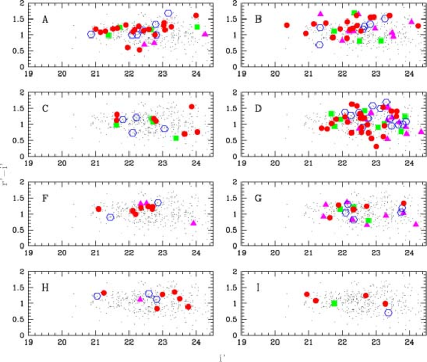
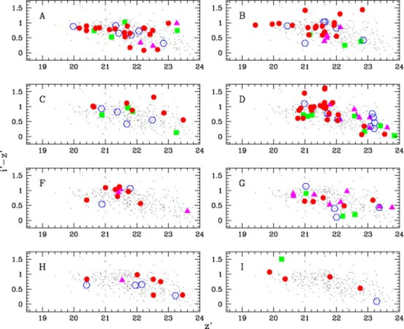
Figure 8: The $(r^{\prime}-i^{\prime})$ vs. $i^{\prime}$ (left) and $(i^{\prime}-z^{\prime})$ vs. $z^{\prime}$ (right) CMDs for eight of the clusters in Cl1604. Small black points indicate all supercluster members. Large red dots are galaxies determined to be members of each specific cluster at radii $r<0.5h^{-1}_{70}$ Mpc. We plot open blue hexagons for galaxies at $0.5<r<0.75h^{-1}_{70}$ Mpc, filled green squares for $0.75<r<1.0h^{-1}_{70}$ Mpc, and filled magenta triangles for $1.0<r<1.5h^{-1}_{70}$ Mpc from the cluster center.

Figure 8 shows the $(r^{\prime}-i^{\prime})$ vs. $i^{\prime}$ and $(i^{\prime}-z^{\prime})$ vs. $z^{\prime}$ CMDs for each of the clusters (note that E is excluded; see §4.1.1) in Cl1604 using only objects determined to be photometrically clean in the ground-based LFC and COSMIC imaging. Small black points indicate all galaxies in the full imaged area having redshifts consistent with supercluster membership ($0.84\leq z\leq 0.96$). Large red dots are galaxies determined to be members of each specific cluster at radii $r<0.5h^{-1}_{70}$ Mpc. We plot open hexagons for galaxies at $0.5<r<0.75h^{-1}_{70}$ Mpc, filled squares for $0.75<r<1.0h^{-1}_{70}$ Mpc, and filled triangles for $1.0<r<1.5h^{-1}_{70}$ Mpc from the cluster center.

First, we note that the photometric errors are significant for fainter galaxies. At $i^{\prime}\sim 24$, for instance, the typical error is 0.1^mag; added in quadrature with another band, we expect at least 0.15^mag of scatter at $i^{\prime}\sim 24$ from photometric uncertainties alone. The intrinsic width of the red sequence, due to age differences at fixed galaxy mass, is only $\sim 0.05^{\rm mag}$ in clusters at $z\sim 1$ (Homeier et al., 2006; Mei et al., 2006), similar to that observed locally (McIntosh et al., 2005). The expected slope of the red sequence, a consequence of metallicity changes with galaxy mass, is also small, of order $-0.05$ (Kodama & Arimoto, 1997). Thus, our ground based observations are not sufficiently accurate to measure these quantities.

Nevertheless, a few general observations are possible. The red sequence is most prominent in Clusters A and B, which also have the highest velocity dispersions, consistent with the morphology-density and color-density relations (Dressler, 1980; Smith et al., 2005; Nuijten et al., 2005; Cooper et al., 2007) and its disappearance in low density environments by $z\sim 1$ (Tanaka et al., 2004). Cluster D, with a velocity dispersion only 5% lower than Cluster A, shows a distinctly less pronounced red sequence. This is illustrated in Figure 9, which shows the distribution of $r^{\prime}-i^{\prime}$ colors for spectroscopically confirmed members of Clusters A and D. The left panel shows galaxies with $r^{\prime}\leq 23.4$, the depth of the complete LRIS spectroscopy in A and D. At these magnitudes, red galaxies have $i^{\prime}\leq 22.6$, with photometric errors of $\sim 0.04^{\rm mag}$ in $r^{\prime}$ and $\sim 0.03^{\rm mag}$ in $i^{\prime}$, or color errors of $\sim 0.05^{\rm mag}$. The right panel shows fainter galaxies, with $23.4<r^{\prime}<25$, where the errors are much larger. The solid histograms indicate galaxies in A, while the dotted line is for Cluster D. The excess of bluer ($(r^{\prime}-i^{\prime})\sim 0.9$) galaxies in Cluster D is evident, especially in the fainter population.

Looking at the left panel, Cluster A has eleven luminous red ($1.0\leq r^{\prime}-i^{\prime}\leq 1.4$) galaxies, while Cluster D (Cl1604+4321), although apparently rich, has only six. If we examine the most luminous objects, the brightest red galaxy in D has $r^{\prime}=22.985$; Cluster A has five more luminous galaxies, extending to $r^{\prime}=22.18$. The lack of luminous red galaxies coupled with the presence of numerous bluer galaxies in D results in a dilution of the red-sequence, making it appear much less prominent than in Cluster A. Clusters A and D have magnitude-limited spectroscopy for all objects with $R<23.5$ from the Oke, Postman, & Lubin (1998) LRIS fields, covering a $6^{\prime}\times 8^{\prime}$ area ($2.8\times 3.7h_{70}^{-1}$ Mpc) around each cluster, so the differences in the luminous galaxy populations between A and D are certainly real and not selection effects.

The absence of luminous galaxies in D is also not an effect of simply having fewer galaxies as a result of its lower velocity dispersion (mass); Cluster A has 1.8 times as many objects with $r^{\prime}<23.4$ and $1.0\leq(r^{\prime}-i^{\prime})\leq 1.4$, while we would expect only $\sim 10\%$ more if we assume $M\propto\sigma^{2}$ and $N_{gals}\propto M$. The discrepancy only gets worse if we look at the most luminous galaxies ($r^{\prime}\leq 23.0$), where there are five times more in A than in D. To explain this as purely a result of A’s large mass, we would have to increase the dispersion of A by $2\sigma$ while at the same time decreasing D’s dispersion by $2\sigma$, resulting in a mass ratio of 4.8, comparable to, but still lower than, the factor of five difference in luminous red galaxies.

Similarly, the fainter galaxy population differences between A and D are also physical, as they are sampled by both second-epoch LRIS and later DEIMOS slitmasks, with similar coverage. Our findings are consistent with the HST results of Homeier et al. (2006), who had fewer redshifts but more precise photometry. Combined with its elongated morphology, these data suggest that Cl1604+4321 (D) is a cluster in the process of formation, and therefore has not yet had time to build up its red sequence and assemble massive red galaxies. The remaining structures have insufficient spectral coverage or too few members with clean ground-based imaging to make conclusive statements about their galaxy populations.

However, it is clear that many galaxies in the supercluster are associated not with the individual clusters but with the connecting filaments instead. This implies that studies of the cluster CMR at high redshift that rely on purely photometric data may overestimate the width of the red sequence due to contamination by dynamically dissociated galaxies. Estimates of the blue galaxy fraction may be similarly compromised. Studies of low-redshift superclusters have also found that $\sim 30\%$ of supercluster members are not associated with specific clusters (Small et al., 1998); this fraction will only increase at larger lookback times as the structures are less collapsed.

4.2 Three Dimensional Supercluster Structure

As noted above, many galaxies in the redshift range of the supercluster are not associated with any of the clusters/groups. We use our entire redshift catalog of 413 Q$>2$ confirmed members to construct a three-dimensional map of the supercluster. To produce this map, we assume that individual galaxy redshifts directly reflect the position of the galaxy within the structure. This is not strictly correct, since the clusters within the structure can have significant velocities relative to the Hubble flow, and the galaxies within the clusters also have their own peculiar velocities. However, we have no other data to constrain the dynamics within this region. If the structure is bound, then the clusters themselves may have significant peculiar velocities within the supercluster, further complicating any dynamical analysis. The redshift depth of the supercluster, taken at face value, implies a radial length of order $100~{}h_{70}^{-1}~{}{\rm Mpc}$, while the transverse size (using Clusters A and J) is only $\sim 13~{}h_{70}^{-1}~{}{\rm Mpc}$.

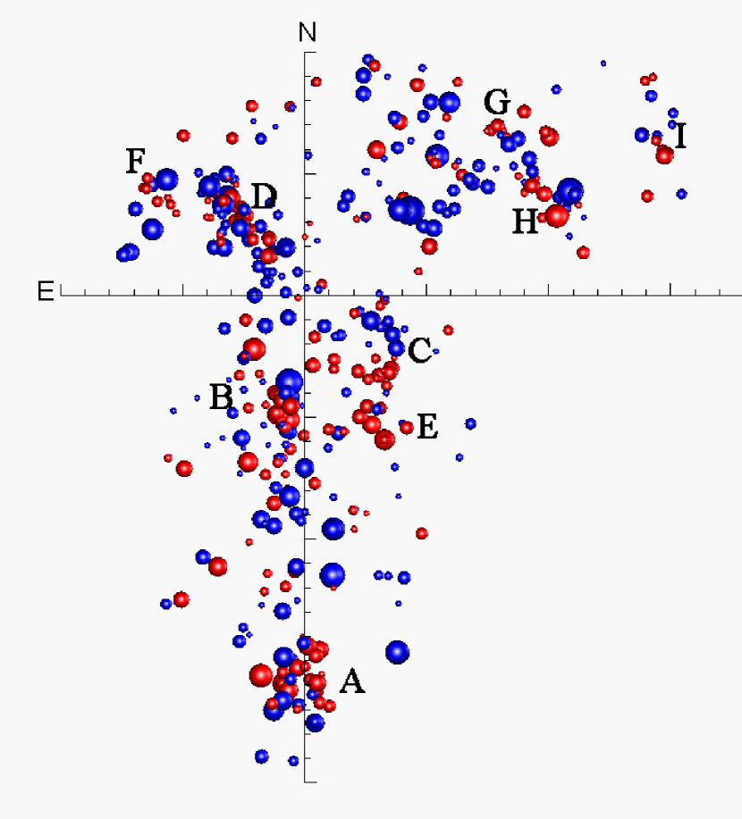
Figure 10: Face-on (xy) view of the Cl1604 supercluster. We show red and blue galaxies, divided at $(i^{\prime}-z^{\prime})=0.7$, as correspondingly colored spheres. Each sphere is scaled by the observed $i^{\prime}$ luminosity of the galaxy.

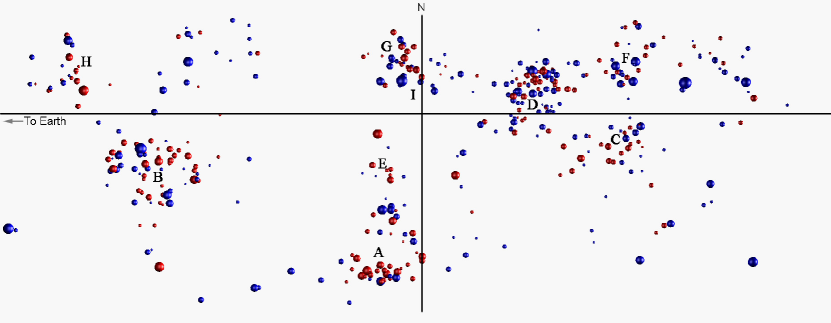
Figure 11: Radial (yz) view of the Cl1604 supercluster. We show red and blue galaxies, divided at $(i^{\prime}-z^{\prime})=0.7$ as correspondingly colored spheres. Each sphere is scaled by the observed $i^{\prime}$ luminosity of the galaxy.

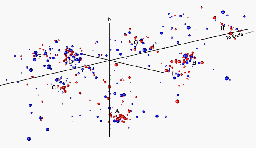
Figure 12: Rotated view of the Cl1604 supercluster. We show red and blue galaxies, divided at $(i^{\prime}-z^{\prime})=0.7$ as correspondingly colored spheres. Each sphere is scaled by the observed $i^{\prime}$ luminosity of the galaxy.

Figures 10,  11 and  12 show three views of the supercluster. Because of the nearly 8:1 axis ratio, we have compressed the radial axis by a factor of five. We show red and blue galaxies, divided at $(i^{\prime}-z^{\prime})=0.7$ as correspondingly colored spheres. Each sphere is scaled by the observed $i^{\prime}$ luminosity of the galaxy. Figure 10 shows the face-on view of the supercluster, as observed on the sky. Clusters A, B and D can be clearly seen. The large red galaxy population in A is evident, as is the elongation of Cluster D. Figure 11 shows the radial distribution of galaxies in Cl1604 as a function of declination. The individual clusters are clear, along with the large number of intercluster galaxies. Color segregation is easily seen, although luminous red galaxies do exist far outside the cluster centers, and luminous blue galaxies are present in the lower-mass clusters and groups. The most luminous blue galaxies are almost exclusively found in the filaments, far from the cluster cores. There are also large voids in the overall galaxy distribution, consistent with the structures seen in large simulations. Finally, Figure 12 shows a rotated view of the supercluster, making its overall structure clearer. From these figures it appears that Cluster B at $z=0.8656$ is relatively isolated from the rest of the supercluster. Determining whether it is actually bound to the overall structure or a more isolated foreground object will require detailed $N$-body simulations mimicking this supercluster.

5 Fore- and Background Structures

Besides the supercluster, a variety of apparent fore- and background structures can be seen in Figure 5. We apply three different criteria to identify coherent overdensities in both redshift and in projection. Candidate structures are selected by taking each galaxy with a measured redshift as a seed, and searching for peaks both in redshift and in projection. We look for groups of galaxies that meet at least one of the following three requirements:

• A. 15 or more concordant redshifts within $\Delta z=0.01$, no spatial requirement

• B. 5 or more concordant redshifts within $\Delta z=0.01$ and within a $0.5h^{-1}_{70}$Mpc radius

• C. 5 or more concordant redshifts within $\Delta z=0.01$ and within a $1.0h^{-1}_{70}$ Mpc radius

The redshift interval of $\Delta z=0.01$ used in peak selection corresponds to a velocity width of $\sim 1500$ km s^-1, broader than the expected dispersion of all but the most massive clusters, and is identical to the criterion of Gilbank et al. (2007). Criterion A includes structures like walls or filaments which might be rejected by the latter. Criteria B and C more closely match other surveys that do spectroscopic followup in a limited spatial region around candidate clusters. Criterion A selects a total of 18 redshift peaks outside the supercluster redshift range. Criterion B selects 6 peaks, all of which are also found by A, while Criterion C selects 13 peaks, 11 of which are also selected by A. Although these candidate structures are chosen based on well-defined criteria, the uneven spatial coverage, survey depth, color selection, and biases such as easier identification of emission-line objects imply that this sample is neither complete nor unbiased (in redshift or galaxy type).

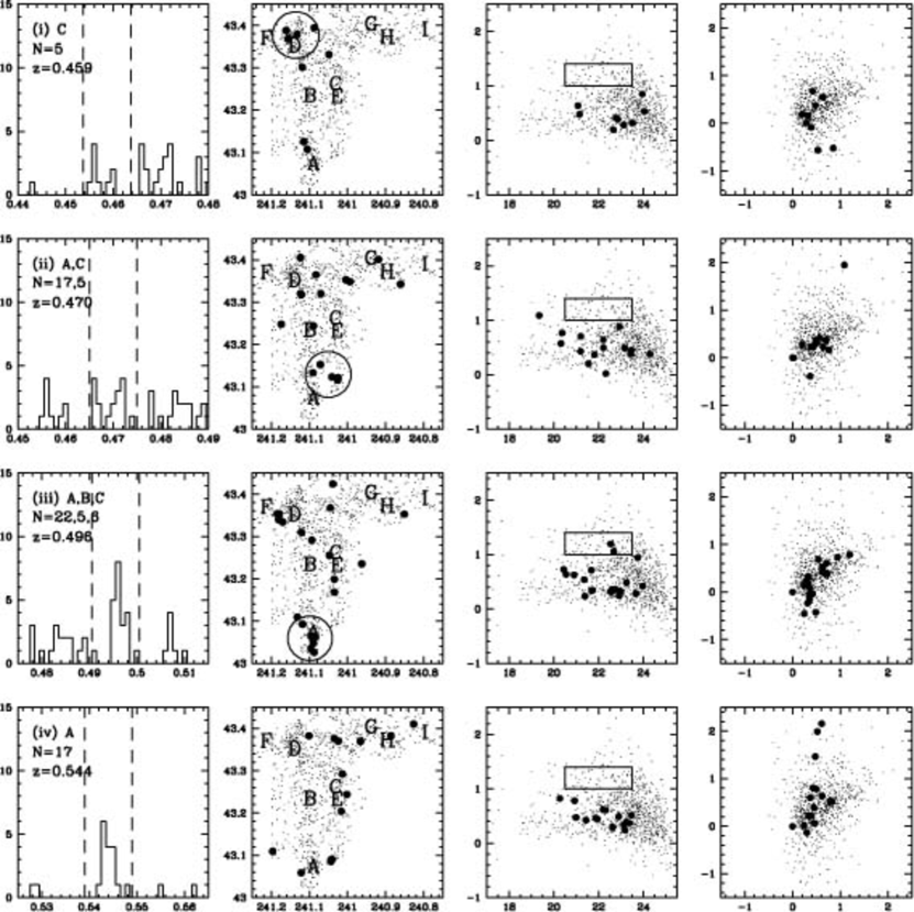
Figure 13: The spatial distributions and CMRs of galaxies in each fore- and background redshift peak. Each row corresponds to a different peak in the redshift histogram, starting at $z\sim 0.4$. The first column shows the redshift histogram in the region of the specific redshift peak, with dashed lines demarcating the redshift range used to plot galaxies in the spatial and color distributions. The left panel includes a Roman numeral corresponding to the structures tallied in Table 2, the number of galaxies in the peak, and the redshift. The second column shows the projected distribution of galaxies in the redshift peak (large dots) overlaid on the overall distribution of spectroscopic objects. Cl1604 components A-J are marked. For redshift peaks that appear to be real structures, a circle of radius 1.5 $h^{-1}_{70}$ Mpc is drawn around the structure centroid. The third column presents the $r^{\prime}-i^{\prime}$ vs. $i^{\prime}$ CMD with all photometric objects as small black dots and the members of each structure as large red dots. A black rectangle outlines the color and magnitude range used in making the density map. The fourth column shows the $r^{\prime}-i^{\prime}$ vs. $i^{\prime}-z^{\prime}$ color-color diagram using the same symbols.

Whether or not these structures are real or artifacts of our color selection and spatial sampling requires looking in greater detail at the spatial distributions and CMRs of galaxies in each apparent redshift peak. These are plotted in Figures 13a-e. Each row corresponds to a different peak in the redshift histogram, starting at $z\sim 0.4$. The first column shows the redshift histogram in the region of the specific redshift peak, with dashed lines demarcating the initial redshift range $\Delta z=0.01$ used to select the peak with Criterion A. The left panel includes a Roman numeral corresponding to the structures tallied in Table 2, followed by letters denoting which criteria are met by the peak. We also show the number of galaxies in the peak based on each of the criteria by which it is selected. The median redshift is included, again using all Criterion A galaxies. The second column shows the projected distribution of galaxies in the redshift peak (within $\Delta z=0.01$) as large dots overlaid on the overall distribution of spectroscopic objects. The locations of Clusters A-I are labeled. If there is an apparent projected overdensity of objects as defined by Criteria B and/or C, we plot a circle of radius $1.0h^{-1}_{70}$ Mpc around the structure centroid, using the mean positions of the galaxies within the apparent projected overdensity (except for structure vii, as detailed below). When there are multiple spatial overdensities in a single redshift peak meeting Criteria B and/or C, we show only the one with the most members. The third column presents the $(r^{\prime}-i^{\prime})$ vs. $i^{\prime}$ color-magnitude diagram with all photometric objects as small black dots and the structure members (based on Criterion A) as large dots. The color and magnitude limits for galaxies used in making the density map are shown as the black rectangle in these panels; the highest priority DEIMOS targets have these colors but extended to $i^{\prime}=24$. The fourth column shows the $(r^{\prime}-i^{\prime})$ vs. $(i^{\prime}-z^{\prime})$ color-color diagram using the same symbols. Redshifts and positions are shown for all spectroscopic objects, while photometric data points are shown only for those objects with clean ground-based photometry to avoid incorrect colors.

Table 2 provides information for all twenty of these redshift peaks. Column 1 gives the Roman numeral identifier of the peak. Columns 2 and 3 give the J2000.0 coordinates. For peaks selected only by Criterion A, the coordinates are the mean of all galaxies in the $\Delta z=0.01$ window; because this criterion does not require a spatial concentration, the coordinates are not necessarily reflective of any true structure center. For peaks selected by Criteria B and/or C, we use the mean coordinates from the galaxies within the overdensity defined by Criterion C, which is most likely to provide a meaningful position. Column 4 lists which criteria were met by each peak, while Column 5 gives the median redshift using all Criterion A galaxies. Columns 6, 7 and 8 give the number of galaxies meeting Criteria A, B and C, respectively.

Figure 13 shows a remarkable diversity of structures. Some are apparently chance projections or collections of galaxies at very similar redshifts but with no clear physical association. These types of objects are likely to be selected by Criterion A but not by B or C, and include structures iv, xiii, xvi and xvii. Seven out of 20 redshift peaks meeting any of our criteria, or 35%, fall into this category. These could be sparse walls or filaments crossing our field, or simple statistical fluctuations. As noted earlier, the uneven spatial sampling, sparse coverage in some areas, and changes in targeting priority make it difficult to model the likelihood of these being real structures without using a full cosmological simulation. Other structures are more clearly filaments or walls, and there are distinct clusters/groups as well. We discuss simple estimates of the false detection rate in Section 5.2.

5.1 Individual Redshift Peaks

We briefly describe each of the structures selected by our three criteria, including their potential effects on the photometric detection of Cl1604 components.

1. Selected only by Criterion C, there is a concentration of five galaxies within 1 $h^{-1}_{70}$ Mpc near Cluster D, and only nine within this redhift peak anywhere in the field. Most of the galaxies in this peak were observed in the original LRIS survey of Oke, Postman, & Lubin (1998). The colors of these six galaxies reveal no clear red sequence, so this is not likely to be a real structure.

2. Although galaxies in this peak meet both Criteria A and C, there is no unambiguous compact, physical structure. Examining only the 11 galaxies in the larger subpeak at $0.468<z<0.474$ highlights the small clump north of Cluster A. Interestingly, most of the galaxies in this peak are H$\beta$ and [OIII] emitters as seen in DEIMOS spectra.

3. There are two strong concentrations of galaxies associated with this redshift peak. In the south, there are 8 galaxies, 7 of which are within a 1 $h^{-1}_{70}$ Mpc radius, most of which have spectra from the original LRIS survey of Oke, Postman, & Lubin (1998). These eight galaxies have $<z>=0.4961$. In the north, there are 6 galaxies within a 1 $h^{-1}_{70}$ Mpc radius near Clusters D and F, mostly with DEIMOS spectra, and $<z>=0.4967$. The coordinates and dispersion reported in Table 2 are derived using only the ten galaxies in the southern clump.

4. Selected only by Criterion A, these galaxies are scattered throughout most of the field. There is no identifiable group or cluster, despite the modest number of galaxies and the well-defined shape of the peak. Again, almost all of the galaxies in this peak are H$\beta$ and [OIII] emitters as seen in DEIMOS spectra.

5. Identified by Criterion C, there are 8 galaxies in the $\Delta z=0.01$ window. The five galaxies meeting Criterion C are mostly concentrated in a tight structure only $38^{\prime\prime}$ or 240 $h^{-1}_{70}$ kpc across.

6. One of the most interesting structures, this appears to be a filament running almost directly N-S in front of the supercluster. It has a low, group-like velocity dispersion of $\sigma=328$ km s^-1, while showing a significant red sequence. Nearly 80% of the peak members have DEIMOS redshifts; the lack of galaxies in the western part of the mapped field is therefore not likely due to lack of coverage. We report the median coordinates and dispersion using all 39 members in the $\Delta z=0.01$ window, although there is no clear center to this structure, and many subclumps that meet Criteria B and/or C. The reddest members of this structure meet our color criteria for the density map, likely enhancing the detectability of Cl1604.

7. These galaxies are isolated in the northeast corner of the field, and the majority have redshifts from the Oke, Postman, & Lubin (1998) survey and would not meet our current color criteria. However, the lack of galaxies at the same redshift near Cluster A, where there is also heavy LRIS coverage, suggests that this structure is spatially isolated.

8. A tight clump of five galaxies is located near Cluster G. Four out of five of these galaxies have colors falling within our red galaxy criteria for density mapping, enhancing the detectability of Cluster G. The four galaxies in closest proximity to each other are within $\Delta z=0.0025$, or $\sim 400$ km s^-1, suggestive of a small group.

9. Detected by all three criteria, there is a concentration of 11 galaxies within a 1 $h^{-1}_{70}$ Mpc radius, centered near Cluster D. Almost all are from the Oke, Postman, & Lubin (1998) survey. These 11 galaxies span a velocity range of only $\sim 600$ km s^-1 with $<z>=0.696$. They yield a velocity dispersion of $\sigma_{biwt}=218\pm 49$ km s^-1, commensurate with being a small group. Again, some of these galaxies meet the red galaxy color cut, enhancing the detectability of Cluster D.

10. A similar structure to the previous one. The large concentration of 16 galaxies with $<z>=0.7284$ near Cluster H contains only objects with DEIMOS redshifts, many of which have red colors. They have a velocity dispersion of $\sigma_{biwt}=285\pm 88$ km s^-1, typical of small groups.

11. The redshift distribution shows multiple peaks within the $\Delta z=0.01$ selection window, and at least two spatial concentrations in the spatial distribution. Just south of clusters B and E we see 17 galaxies with $<z>=0.775$ within a 1.6 $h^{-1}_{70}$ Mpc radius. They have a velocity dispersion of $\sigma_{biwt}=352\pm 82$ km s^-1, typical of small groups. In the northwest, between Clusters H and I, there are 8 galaxies in a 1.25 $h^{-1}_{70}$ Mpc radius. This clump has a mean redshift of $<z>=0.781$. Unsurprisingly, a majority of these galaxies have red colors that fall within our selection window, since their redshifts are quite similar to that of the supercluster.

12. An extremely narrow redshift peak, there may be a small group near Cluster G, selected by Criteria B and C. Even using all galaxies in the peak gives a dispersion of only 133 km s^-1.

13. Selected only by Criterion A, these galaxies are scattered throughout most of the field. There is a concentration just west of Cluster D, but insufficient to meet either of the spatial criteria. Since galaxies at this redshift would have colors strongly sampled by DEIMOS, and the region near Cluster D has extensive LRIS spectroscopy as well, it is unlikely that there is a significant structure associated with this peak.

14. A possible structure near Cluster D. There are 10 galaxies in this region, with $<z>=0.822$ and $\sigma_{biwt}=220\pm 142$ km s^-1. Most of the galaxies are red and seem to form a red sequence. As with the previous structure, the spectroscopic sampling in this area is very dense, so it is unlikely that we have missed many of the luminous red members of this structure.

15. A small clump near Cluster A. All of the galaxies in the tight clump are from the Oke, Postman, & Lubin (1998) survey.

16. Only selected by Criterion A, the redshift and spatial distributions show no evidence for a group.

17. Only selected by Criterion A, the redshift and spatial distributions show no evidence for a group, except for a possible concentration in the northern end of the field.

18. Although meeting both Criteria A and C, there is no obvious single overdensity, and the redshift distribution is quite broad.

19. Although the redshift distribution is broad, we see a very compact group north of Cluster C, and this peak meets all three selection criteria. The 9 galaxies in this clump are contained in a region of radius $0.4h^{-1}_{70}$ Mpc. They have $<z>=1.179$ and $\sigma_{biwt}=289^{+40}_{-92}$ km s^-1. This structure seems to be a low mass group.

20. A group or poor cluster at $z=1.207$. The majority (12) of the galaxies are concentrated in a $1.5\times 2.5h^{-1}_{70}$ Mpc region in the northeast corner of the observed area, whose center we have marked on the plot. The velocity dispersion from these 12 galaxies is $288\pm 82$ km s^-1. All of these galaxies are very faint ($i^{\prime}>23$) and are detected spectroscopically from their OII emission alone, consistent with their broad range in colors. If the velocity dispersion is reflective of the group mass, this is the highest redshift group of such low mass known.

From the third column in Fig 13 we see that many of the structures, especially at $z\sim 0.7$, contain significant numbers of galaxies with colors consistent with supercluster membership. Some of these show projected density peaks near components of the supercluster, which likely contributed to the detectability of low-mass groups and filaments in the region. Narrowing the color range slightly would not eliminate their contributions to the density map. The CMDs and redshift distributions of the structures demonstrate the difficulty of establishing the physical nature of moderate-mass, high-redshift systems.

5.2 Are Such Structures Real Physical Associations ?

It is extremely common practice to detect clusters with some photometric technique, and report as few as three redshifts for confirmation. For instance, Olsen et al. (2005) examined spectroscopy in the fields of five $z>0.6$ clusters in the ESO Imaging Survey (EIS) Cluster Candidate Catalog, and found numerous groups in many of the fields, often with only three concordant redshifts (such as EISJ0046-2951). They find multiple redshift peaks in some of their fields, and rely on the alignment of galaxies in each redshift peak with the location of the candidate derived from the initial imaging to determine confirmations and assign redshifts. They do not specify a minimum area within which these three redshifts had to be found (with statistical significance tests relying purely on redshift distributions with no spatial information), nor detail the spectroscopic completeness (especially as a function of color), making statistical statements impossible. However, inspection of their figures shows that these objects were typically within a $\sim 2$ arcminute diameter region inside the large spectroscopic field. Similarly, Gilbank et al. (2007) performed follow-up observations of RCS (Gladders & Yee, 2005) clusters, and often found only 3-5 concordant redshifts for the candidates. They follow the arguments of Gilbank et al. (2004), similar to those of Holden et al. (1999) and Ramella et al. (2000), to conclude that finding just three concordant redshifts for early type galaxies in a field with 5 arcmin radius at $z=0.3$ results in a $\sim 99\%$ likelihood of having a true structure. This radius corresponds to $\sim 2$ arcminutes at $z=1$.

To qualitatively assess the reliability of cluster confirmation using so few concordant redshifts, we examined each of our redshift peaks which meet only Criterion A, and not Criteria B or C. There are 7 such peaks comprising $\sim 35\%$ of our candidates. This provides a sample of galaxies that are in redshift peaks but not contained in any obvious spatial structure. We could simply assume that all of these are projections, implying that requiring no spatial coincidence results in at least a $35\%$ false positive rate for cluster confirmation. We caution that even candidate structures meeting Criteria B or C may be projections (which would imply an increase in the false positive rate), and that some structures that only meet Criterion A may be real (decreasing the false positive rate). As noted earlier, applying our spectroscopic selection in detail to large cosmological simulations with realistic galaxy distributions and colors is needed to definitively understand the nature of the detected structures.

To compare more directly with the studies mentioned above, we must account for our higher redshift sampling. For instance, Olsen et al. (2005) have 266 redshifts in 5 fields. They do not provide the area coverage of their spectroscopy, so we estimate a spectroscopic area coverage of $\sim 150$ sq. arcmin based on their figures, or a redshift density of $\sim 1.75$ per sq. arcmin. This compares to our 1138 redshifts in $\sim 300$ sq. arcmin, a sampling rate of 3.8 per sq. arcmin. Excluding the LRIS redshifts, which cover small regions around Clusters A and D, we have 3.0 redshifts per sq. arcmin. Our redshift sampling is indeed greater by a factor of $\sim 2$. Our area coverage is also a factor of $\sim 2$ greater. However, we require five times more galaxies in each peak (15 as opposed to 3), approximately compensating for these factors. Thus, our estimated 35% false positive rate may be indicative of the rate expected in Olsen et al. (2005). If instead we reduce our requirement to account purely for the difference in sampling, we need only $\sim 5$ galaxies per peak, but contained within a region comparable to the spectroscopic fields of Olsen et al. (2005), about $5^{\prime}\times 5^{\prime}$. This yields 22 candidate peaks, and they are almost identical to those found from our full area and requiring 15 galaxies in the peak, suggesting that our false positive rate is reasonable. Comparison to Gilbank et al. (2007) is more difficult, since they do not provide information on the effective area covered in each field, magnitude limits, or color selection. However, examination of their Fig. 2 shows numerous cases where there is no obvious redshift peak, especially for fields that are poorly sampled. We also consider how rapidly the number of candidates increases with area for a fixed number of galaxies per redshift peak. Our original Criterion B requires 5 concordant galaxies within a $0.5h^{-1}_{70}$Mpc radius; the typical area covered is 5 sq. arcmin. Similarly, Criterion C encompasses $~{}\sim 17$ sq. arcmin on average, while the EIS area is 25 sq. arcmin. We find 6, 13, and 22 candidates using these search areas, respectively. Visual inspection of Fig. 13 suggests that even Criterion C may yield structures that are not obviously physical associations, and sampling even larger areas and requiring fewer than five concordant redshifts can only exacerbate this problem.

Alternatively, the redshift peaks in our data showing minimal spatial structure (i.e., meeting only Criterion A) provide a test sample to estimate the likelihood of false positives from small projected galaxy groupings. To do this, we examine each galaxy in each of the redshift peaks selected only by Criterion A. For each galaxy, we count the number of neighbors within 0.25, 0.5 and 2 $h^{-1}_{70}$ Mpc radii (31”, 62”, 4.13’ at $z=1$). We then count how many projected groupings of $N_{near}>3$ galaxies are present for each peak, mimicking some of the selections used in other surveys. Using the smallest radius, 3 out of 6 redshift peaks have a group of at least 3 galaxies within the required area. Increasing the test radius to 0.5 $h^{-1}_{70}$ Mpc results in all but one of these redshift peaks containing a group of three or even four nearby galaxies. For the largest test radius, every redshift peak contains at least three and as many as five distinct groups, and these groups typically have 6-11 members. These results suggest that, with our sampling, requiring only 3 galaxies even in a very small area is likely to produce false structures. At the largest radius (2 $h^{-1}_{70}$ Mpc) we are covering areas similar to those in Olsen et al. (2005) and Gilbank et al. (2007). Adjusting for the lower sampling in Olsen et al. (2005), nearly all of our Criterion-A-only peaks would have 3 concordant redshifts within a comparable field size. However, only one of these peaks would have 4 or more concordant redshifts. This simply reflects the fact that sparse spectroscopic sampling over modest regions can easily produce spurious redshift peaks.

We note that this analysis includes not just red sequence galaxies, since in some cases we do not sample the RS at the redshift of the peak. This may increase the likelihood of finding chance projections. If we required instead a small number of concordant redshifts and that these objects were also along the red sequence, we would have many fewer candidates and eliminate many potentially spurious groups. However, most spectroscopic follow-up studies do not impose such a requirement. In addition, for poor groups, we might not expect to see a strong red sequence at redshifts like those studied here, so requiring a red sequence might eliminate otherwise physical structures. Our analysis also does not consider the alignment of small redshift peaks with cluster candidates pre-selected using photometric redshifts or red sequence techniques. The likelihood of finding a redshift peak with $N\sim 3$ galaxies at the location of a cluster candidate and with redshift comparable to the photometric estimate is certainly much lower than finding a peak at any redshift along the line of sight. However, we have shown that in a modest field, it is easy to find peaks with $N\sim 3$ galaxies at almost any redshift, so using such data to confirm candidate clusters is questionable.

A competing effect is low spectroscopic completeness, decreasing the likelihood of finding close projections. If we use simple criteria of three galaxies within a velocity window of $\pm 3000$ km s^-1 and a radius of 0.25 $h^{-1}_{70}$ Mpc, every redshift peak along the line-of-sight would qualify as a physical structure. While this may be true, it is unlikely. Given the complex sampling, we would have to replicate our observations on large mock galaxy catalogs to give correct likelihoods for each structure. This problem will persist for surveys like ORELSE, and for large sky surveys such as Pan-STARRS and LSST, where spectroscopic followup of complete samples of faint, distant galaxies will be difficult.

6 Discussion

6.1 Implications for Lensing and Cosmology

Detection of high-redshift clusters using photometric techniques can be affected by line-of-sight projections over radial distances comparable to the redshift resolution of simple color-based techniques. Cohn et al. (2007) show that many clusters detected in a red-sequence type survey at $z\sim 1$ are made up of galaxies from multiple distinct cluster-size dark matter halos. Their work does not include smaller groups, of which we expect to find many in the infall regions of high-redshift clusters. They also demonstrate that the problem becomes substantially worse at $z\sim 1$ than it is at $z\sim 0.5$, in part because a fixed pair of filters cannot sample features such as the 4000Å  break over such a broad redshift range.

We find many small groups in both the fore- and background of the target structure at $z\sim 0.9$. Examination of model galaxy tracks from Bruzual & Charlot (2003) in the $r^{\prime}-i^{\prime}$ vs. $i^{\prime}-z^{\prime}$ color-color space for both galaxies with a single burst at $z=3$ and the RCS model (a 0.1 Gyr burst ending at $z=2.5$ with a $\tau=0.1$ Gyr exponential decline thereafter) shows that colors for galaxies over a moderately broad redshift range ($z\sim 0.8-1.2$) are quite similar, with the differences in color comparable to ground-based photometric errors (ORELSE I). Therefore, any survey relying on only two- or three-color moderate-depth ground-based imaging is subject to this type of confusion. The surveys will be biased toward detecting projected systems, the same problem that has plagued lower redshift optical cluster catalogs (Katgert et al., 1996). Even with large cosmological simulations, the detailed effects of such projections on cluster detection, number counts, and mass estimates will be difficult to quantify. The most recent studies (Cohn et al., 2007) using the Millennium Simulation and a red-sequence cluster finder are still hampered by the inability of simulations to reproduce the observed colors of cluster galaxies. Extensive spectroscopy of at least a subset of clusters found using optical and X-ray surveys is needed to understand the contamination rates, redshift distributions, substructure, and other cluster properties; such work is only now under way (Gilbank et al., 2007).

Given that such projections can only enhance the detectability of lower mass systems, as well as inflate velocity dispersions and increase the weak lensing signal, mass estimates for single bound cluster components using such techniques will always tend to be overestimated. A striking example is Cluster A (Cl1604+4304), whose initial velocity dispersion estimate was 1200 km s^-1 (Postman, Lubin, & Oke, 2001). Adding many more spectra, but not tightly restricting the area sampled, Gal & Lubin (2004) found $\sigma=700$ km s^-1. We now find that the velocity dispersion can be as low as $\sigma=532$ km s^-1, more than a factor of two below the initial measurement. Comparison of velocity dispersions derived using a variety of galaxy subpopulations (as done in §4.3) with simulations is necessary to determine the optimal mass tracer.

Hoekstra (2003) suggested that structures associated with, but not bound to, a cluster can increase errors in lensing mass estimates twofold. Our data shows that such filaments may be common at $z\sim 1$. Furthermore, completely independent structures along the line-of-sight can be cause for concern, even at low redshift (Łokas et al., 2006). In Cl1604, we find moderate-mass groups at $z\sim 1.2$ directly projected onto clusters at $z\sim 0.9$. Both types of structures can affect the derived mass profiles. Typically, NFW profiles (Navarro et al., 1996) are fit to clusters in both observations and simulations; clusters have been observed with NFW concentrations c incompatible with simulated clusters. Very recent simulations of weak lensing by clusters plus foreground group-size halos (King & Corless, 2007) demonstrates that line-of-sight contamination by even low-mass systems can both decrease and increase the measured value of c, depending on the geometry. It is not yet known how much this can affect the overall distribution of observed concentrations and masses from weak lensing. Implementing techniques that incorporate multi-wavelength data (X-ray, Sunyaev-Z’eldovich, optical) can overcome some of these issues, but requires both extensive data and computational power (Mahdavi et al., 2007), limiting it to rich, low-redshift clusters or only the most massive structures at higher redshift for the time being. With somewhat less data, it is possible to compare X-ray and weak lensing masses for clusters. Recent work using observational data has shown moderate agreement between these two techniques, but discrepancies are plentiful and systematic errors are much too large for precision cosmological measurements (Sehgal et al., 2008). In contrast, some lensing simulations claim that high completeness, low contamination, and good mass fidelity can be achieved with weak lensing (Pace et al., 2007), but this has yet to be proven with large samples of real data.

Weak lensing has already been used to estimate the mass of Cl1604+4304 (Cluster A, Margoniner et al., 2005), resulting in a mass of $3.67\pm 1.47\times(R/500kpc)10^{14}M_{\odot}$, corresponding to a velocity dispersion of $1009\pm 199$ km s^-1. This is significantly higher than the $575^{+110}_{-85}$ km s^-1 estimated from the cluster’s X-ray temperature of $T_{X}=2.51^{+1.05}_{-0.69}$ keV (Lubin et al., 2004). The velocity dispersion presented here lies in between these two estimates, but is much more consistent with the X-ray temperature. Earlier work on a much smaller region using HST WFPC2 data suggested multiple mass peaks associated with this structure (Umetsu & Futamase, 2000). Cl1604+4304 is the most isolated component of the supercluster, with the only foreground structures being a group at $z=0.495$ and a possible wall at $z=0.600$. Nevertheless, its estimated mass varies by a factor of nearly two. Improved X-ray measurements from deep Chandra observations (Kocevski et al., 2008) and lensing data from a recent ACS mosaic, combined with our spectroscopic database, may help resolve this discrepancy.

Instead of measuring individual cluster masses, one could avoid some of the above problems with a sufficiently large and deep survey by calculating the mass on very large ($\sim 100$ Mpc) scales over several superclusters, and comparing the results to simulations and structure formation theories, but such surveys remain in the future. With excellent deep photometric data, it is also possible to use weak lensing tomography, incorporating photometric redshifts to map all the galaxies along the line-of-sight. However, even the best photometric redshifts have errors which are equal to or greater than the entire redshift depth of the Cl1604 structure (Margoniner & Wittman, 2008). As a result, uncertainties in the bias and scatter of photo-$z$ estimators with redshift remain a problem (Ma et al., 2006), and will require extensive spectroscopy to calibrate.

Finally, we note that Cl1604 is an optically selected large scale structure. To whatever extent it is not representative of all structures at similar redshifts, any conclusions based on Cl1604 alone may be biased. For this reason, the ORELSE survey has included a variety of structures originally detected using X-ray, optical and even radio techniques. Once the survey is complete, we can address biases due to the cluster detection technique. Within Cl1604, the supercluster members were targeted based on their red colors (see §3), so that the blue galaxy population may be undersampled; nevertheless, $\sim 50\%$ of the targets are outside the red sequence.

6.2 Future Work

The extensive spectroscopic database described here is being used for a variety of projects. Detailed analysis of line strengths as a function of position in the structure, local density, and host cluster properties are being derived by stacking spectra (Lemaux et al., 2008b). The redshift range of the supercluster along with our spectral setup forces the use of the [OII] doublet at 3727Å  as a proxy for H$\alpha$ emission and thus ongoing star-formation activity. Since [OII] has been shown to be a flawed tracer (Yan et al., 2006), we are using near-IR spectroscopy to search for H$\alpha$ emission in a subset of our confirmed supercluster members in order to determine the contribution of non-stellar (i.e. nuclear) sources to the observed [OII] emission. We have also serendipitously detected a significant number of $z>4$ Ly$\alpha$ sources in the DEIMOS data, and their properties will be described in Lemaux et al. (2008a).

A 17-pointing ACS mosaic of the field is being used to examine the CMDs of individual clusters, in the manner of Homeier et al. (2006) and Andreon (2008), who used two earlier pointings centered on Clusters A and D. These images also allow us to compare galaxy colors and morphologies with their spectroscopic properties, and relate them to their location within the supercluster. Deep Chandra observations are being used to map the distribution of AGN within the supercluster and determine the X-ray luminosity (and hence mass) of individual clusters in the complex (Kocevski et al., 2008). Our spectroscopic database, along with our ACS imaging, will allow us to examine the spectral and morphological properties of AGN host galaxies, as well as their local environments, in order to shed light on the mechanisms which trigger nuclear activity in these systems. Deep VLA 1.4GHz mapping of the field shows both bright AGN-like sources and an excess of faint, possibly star-bursting galaxies (Miller et al., 2008). Preliminary results already suggest signs of environmental segregation, with the radio-loud population found in dense regions which the radio-faint and X-ray detected AGN avoid.

Deep Spitzer IRAC and MIPS maps have been obtained, providing both rest-frame K-band luminosities for estimating the stellar mass content of member galaxies, and search for obscured star formation that is becoming more prevalent at higher redshifts. Ground-based K-band imaging is also being used for stellar mass estimation. Combining all of these observations will allow detailed SED fitting and modeling of the star formation histories of supercluster members. For galaxies without spectroscopy, the extensive multi-wavelength data will be used to estimate redshifts photometrically, both as input to lensing models and to better map the supercluster structure.

7 Conclusions

We have presented the results of an extensive spectroscopic campaign to map the Cl 1604 supercluster at $z\sim 0.9$. With over 400 confirmed members, this database provides coverage comparable to studies of local structures, but at a lookback time of 7 Gyr. The large number of redshifts is crucial for confirming the individual clusters, measuring accurate velocity dispersions, and finding contamination due to fore- and background clusters. A three-dimensional map of the supercluster is constructed, making possible the comparison of such structures to large simulations. We also report the discovery of a poor cluster at $z=1.207$ with at least 15 confirmed members within a $\pm 600$ km s^-1 window and $1h^{-1}_{70}$ Mpc radius, making it one of the highest redshift structures selected spectroscopically.

This dataset forms the foundation for a variety of follow-up studies, using many wavelengths to identify preferred sites for inducing and quenching star formation and AGN activity. The extensive spectroscopy allows identification of samples of rare objects, including radio and X-ray sources within the supercluster. Without the large number of redshifts, it is impossible to definitively associate individual objects with the supercluster due to the many sources along the line of sight that are not physically associated with the structure. As an example, Kocevski et al. (2008) and Miller et al. (2008) show that X-ray and radio sources within the supercluster are a very small fraction of the total number of such sources in the field. The same is true for infrared sources such as starbursts. Construction of luminosity functions for these rarer sources has traditionally hampered by the lack of redshifts (Branchesi et al., 2006); our survey is designed to alleviate these problems. The only comparable project is the PISCES program, with deep optical imaging and spectroscopy of high-$z$ clusters with Subaru, but their targets are typically more massive clusters and their spectroscopic followup is much less complete. Field surveys such as GOODS, AEGIS and COSMOS provide similar data to ORELSE, both in terms of multi-wavelength and spectroscopic coverage, but lack the sampling of dense environments. For instance, COSMOS contains just one large scale structure at $z\sim 0.7$ (Guzzo et al., 2007).

Such detailed mapping, encompassing large ($>10$ Mpc) areas will be essential for a statistical sample of clusters over a wide redshift baseline to understand the diversity of structures they are embedded in. The redshift depth of the supercluster is comparable to photometric redshift errors achievable from optical ground based surveys, and especially two-band cluster surveys, potentially enhancing its detectability. At such high redshifts, photometric errors are larger for faint galaxies, photometric redshift errors increase, the change in color of the red sequence with unit $\Delta z$ is reduced (see Fig. 1 of Gladders & Yee, 2005), and clusters are still in the process of merging and accreting their galaxies. All of these effects complicate our ability to reliably construct cluster catalogs over a wide range of redshifts. Future programs relying on photometric redshifts, weak lensing, S-Z, and X-ray data (in particular, luminosities) to estimate cluster masses must understand the biases inherent in each technique, especially when using large samples to constrain cosmological parameters. While large cosmological simulations can provide insight into these issues, their current inability to accurately reproduce galaxy properties, especially colors, means that more observations are necessary. The ORELSE survey will provide such data on a variety of structures at $0.6<z<1.2$, forming an invaluable resource for both galaxy evolution and cosmological studies.

Table 1: Cl1604 Cluster Coordinates, Redshifts and Velocity Dispersions

		J2000.0			Within $0.5h^{-1}_{70}$ Mpc				Within $1.0h^{-1}_{70}$ Mpc				Within $1.5h^{-1}_{70}$ Mpc
ID	Name	RA	Dec		$N$	$z_{mean}$	$\sigma~{}(N_{agree})$		$N$	$z_{mean}$	$\sigma~{}(N_{agree})$		$N$	$z_{mean}$	$\sigma~{}(N_{agree})$
A	Cl1604+4304	241.08946	43.07613		21	0.89838	532$\pm$127 (2)		32	0.89861	619$\pm$96 (3)		36	0.89832	682$\pm$109 (3)
B	Cl1604+4314	241.09890	43.23550		20	0.86574	756$\pm$83 (3)		32	0.86531	811$\pm$76 (3)		47	0.86569	767$\pm$76 (3)
C	Cl1604+4316	241.03162	43.26313		8	0.93451	439$\pm$256 (1)		18	0.93511	313$\pm$41 (3)			$\cdots$	$\cdots$
D	Cl1604+4321	241.13865	43.35343		28	0.92351	559$\pm$171 (2)		53	0.92280	590$\pm$112 (2)		69	0.92340	668$\pm$103 (3)
E	Cl1604+4314B	241.02815	43.23343			$\cdots$	$\cdots$		$\cdots$	$\cdots$	$\cdots$		$\cdots$	$\cdots$	$\cdots$
F	Cl1605+4322	241.21314	43.37091		7	0.93659	142$\pm$297 (1)		9	0.93608	173$\pm$220 (1)		13	0.93532	435$\pm$129 (2)
G	Cl1604+4324	240.93754	43.40520		6	0.89932			13	0.90075	409$\pm$101 (3)		21	0.90210	477$\pm$152 (3)
H	Cl1604+4322	240.89648	43.37309		6	0.85292			10	0.85226	302$\pm$64 (3)		11	0.85243	312$\pm$57 (3)
I	Cl1603+4323	240.79691	43.39176		5	0.90230			7	0.90238	359$\pm$140 (3)		7	0.90238	359$\pm$140 (3)
J	Cl1604+4331	240.91905	43.51648			$\cdots$	$\cdots$		$\cdots$	$\cdots$	$\cdots$		$\cdots$	$\cdots$	$\cdots$

Table 2: Fore- and Background Redshift Peaks

ID	RA (J2000)	Dec (J2000)	Criteria	$z$	NA	NB	NC
i	241.13561	43.37704	C	0.459	$\cdots$	$\cdots$	5
ii	241.05078	43.12914	AC	0.470	17	$\cdots$	5
iii	241.09854	43.05963	ABC	0.496	22	5	6
iv	241.02019	43.24290	A	0.544	17	$\cdots$	$\cdots$
v	240.98975	43.34832	C	0.568	$\cdots$	$\cdots$	5
vi	241.07777	43.26100	ABC	0.599	39	5	9
vii	241.11231	43.38718	ABC	0.620	16	5	8
viii	240.94653	43.39078	AC	0.642	15	$\cdots$	5
ix	241.14468	43.38072	ABC	0.696	21	6	11
x	240.87280	43.40267	AC	0.730	32	$\cdots$	9
xi	241.06424	43.19683	AC	0.777	38	$\cdots$	9
xii	240.94727	43.39270	ABC	0.789	16	5	8
xiii	241.08856	43.30186	A	0.809	15	$\cdots$	$\cdots$
xiv	241.09376	43.33907	A	0.822	21	$\cdots$	$\cdots$
xv	241.09265	43.06344	A	0.829	15	$\cdots$	$\cdots$
xvi	241.06491	43.26877	A	0.971	18	$\cdots$	$\cdots$
xvii	241.05082	43.30216	A	0.982	24	$\cdots$	$\cdots$
xviii	241.09734	43.32171	AC	1.032	22	$\cdots$	5
xix	241.05106	43.30613	ABC	1.177	22	5	8
xx	241.13109	43.35544	A	1.207	15	$\cdots$	$\cdots$

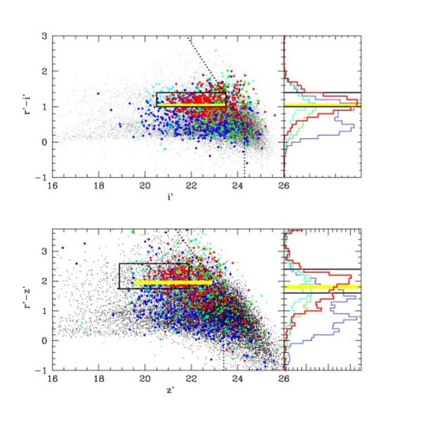
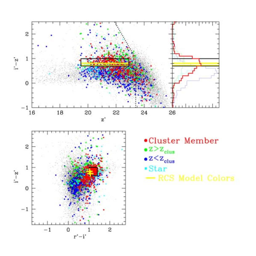
Figure 1: The $i^{\prime}$ vs. $(r^{\prime}-i^{\prime})$, $z^{\prime}$ vs. $(r^{\prime}-z^{\prime})$, $z^{\prime}$ vs. $(i^{\prime}-z^{\prime})$ and $(r^{\prime}-i^{\prime})$ vs. $(i^{\prime}-z^{\prime})$ color-magnitude and color-color diagrams of all objects in our LFC and COSMIC imaging areas. The black rectangular regions outline the color-selections applied to produce the density maps and prioritize spectroscopic targets. The yellow bars and crosses show the synthetic colors for a $z=0.9$ early-type galaxy based on the RCS models; they are within our broad color cut but not an exact fit to the observed colors. Spectroscopically confirmed supercluster members are overplotted as large red dots. Foreground galaxies at $z<0.84$ are shown as blue dots, background galaxies at $z>0.96$ are green dots, and cyan dots are stars. Color distributions of spectroscopic objects are shown to the right of each CMD.

Figure 5: Redshift distribution in the Cl1604 field. The top panel shows all extragalactic objects (dotted line) and only those with high redshift quality (solid line). The bottom panel focuses on the supercluster redshift range with redshift bins of $\Delta z=0.001$.

Figure 9: The distribution of $r^{\prime}-i^{\prime}$ colors for spectroscopically confirmed members of Clusters A and D. The left panel shows galaxies with $r^{\prime}\leq 23.4$, the depth of the complete LRIS spectroscopy in A and D. The right panel shows fainter galaxies, with $23.4<r^{\prime}<25$. The solid histograms indicate galaxies in A, while the dotted line is for Cluster D. The excess of bluer [$(r^{\prime}-i^{\prime})\sim 0.9$] galaxies and lack of luminous red galaxies in Cluster D is evident.

Fig. 13. — Continued.

Fig. 13. — Continued.

Fig. 13. — Continued.

Fig. 13. — Continued.

References

- Adelman-McCarthy et al. (2008) Adelman-McCarthy, J. K., et al. 2008, ApJS, 175, 297
- Andreon (2008) Andreon, S. 2008, MNRAS, 386, 1045
- Beers, Flynn, & Gebhardt (1990) Beers, T. C., Flynn, K., & Gebhardt, K. 1990, AJ, 100, 32
- Bertin & Arnouts (1996) Bertin, E. & Arnouts, S. 1996, A&AS, 117, 393
- Bower et al. (1992) Bower, R. G., Lucey, J. R., & Ellis, R. S. 1992, MNRAS, 254, 589
- Branchesi et al. (2006) Branchesi, M., Gioia, I. M., Fanti, C., Fanti, R., & Perley, R. 2006, A&A, 446, 97
- Bruzual & Charlot (2003) Bruzual, G., & Charlot, S. 2003, MNRAS, 344, 1000
- Cohn et al. (2007) Cohn, J. D., Evrard, A. E., White, M., Croton, D., & Ellingson, E. 2007, MNRAS, 382, 1738
- Cooper et al. (2007) Cooper, M. et al. 2007, in prep
- Davis et al. (2007) Davis, M. et al. 2007, in prep
- Davis et al. (2003) Davis, M., et al. 2003, Proc. SPIE, 4834, 161
- De Filippis et al. (2005) De Filippis, E., Sereno, M., Bautz, M. W., & Longo, G. 2005, ApJ, 625, 108
- Dressler (1980) Dressler, A. 1980, ApJ, 236, 351
- Dressler & Shectman (1988) Dressler, A., & Shectman, S. A. 1988, AJ, 95, 985
- Dressler et al. (2004) Dressler, A., Oemler, A. J., Poggianti, B. M., Smail, I., Trager, S., Shectman, S. A., Couch, W. J., & Ellis, R. S. 2004, ApJ, 617, 867
- Evrard et al. (2002) Evrard, A. E. et al. 2002, ApJ, 573, 7
- Faber et al. (2003) Faber, S. M. et al. 2003, Proc. SPIE, 4841, 1657
- Ford et al. (2003) Ford, H. C., et al. 2003, Proc. SPIE, 4854, 81
- Gal et al. (2008) Gal, R. R., Lubin, L. M., Lemaux, B. C., Kocevski, D. & Squires, G. K. 2008, in prep
- Gal et al. (2005) Gal, R. R., Lubin, L. M., & Squires, G. K. 2005, AJ, 129, 1827
- Gal & Lubin (2004) Gal, R. R. & Lubin, L. M. 2004, ApJ, 607, L1
- Gal et al. (2003) Gal, R. R., de Carvalho, R. R., Lopes, P. A. A., Djorgovski, S. G., Brunner, R. J., Mahabal, A., & Odewahn, S. C. 2003, AJ, 125, 2064
- Gilbank et al. (2008) Gilbank, D. G., Yee, H. K. C., Ellingson, E., Hicks, A. K., Gladders, M. D., Barrientos, L. F., & Keeney, B. 2008, ApJ, 677, L89
- Gilbank et al. (2007) Gilbank, D. G., Yee, H. K. C., Ellingson, E., Gladders, M. D., Barrientos, L. F., & Blindert, K. 2007, AJ, 134, 282
- Gilbank et al. (2004) Gilbank, D. G., Bower, R. G., Castander, F. J., & Ziegler, B. L. 2004, MNRAS, 348, 551
- Gladders & Yee (2000) Gladders, M. D., & Yee, H. K. C. 2000, AJ, 120, 2148
- Gladders & Yee (2005) Gladders, M. D., & Yee, H. K. C. 2005, ApJS, 157, 1
- Goto et al. (2002) Goto, T., et al. 2002, AJ, 123, 1807
- Gunn, Hoessel, & Oke (1986) Gunn, J. E., Hoessel, J. G., & Oke, J. B. 1986, ApJ, 306, 30
- Guzzo et al. (2007) Guzzo, L., et al. 2007, ApJS, 172, 254
- Hoekstra (2003) Hoekstra, H. 2003, MNRAS, 339, 1155
- Holden et al. (1999) Holden, B. P., Nichol, R. C., Romer, A. K., Metevier, A., Postman, M., Ulmer, M. P., & Lubin, L. M. 1999, AJ, 118, 2002
- Homeier et al. (2006) Homeier, N. L., et al. 2006, ApJ, 647, 256
- Horne (1986) Horne, K. 1986, PASP, 98, 609
- Jannuzi & Dey (1999) Jannuzi, B. T., & Dey, A. 1999, Photometric Redshifts and the Detection of High Redshift Galaxies, 191, 111
- Jing & Suto (2002) Jing, Y. P., & Suto, Y. 2002, ApJ, 574, 538
- Katgert et al. (1996) Katgert, P., et al. 1996, A&A, 310, 8
- Kells et al. (1998) Kells, W., Dressler, A., Sivaramakrishnan, A., Carr, D., Koch, E., Epps, H., Hilyard, D., & Pardeilhan, G. 1998, PASP, 110, 1487
- King & Corless (2007) King, L., & Corless, V. 2007, MNRAS, 374, L37
- Kocevski et al. (2008) Kocevski, D., et al. 2008, ApJ, submitted
- Kodama et al. (2005) Kodama, T., et al. 2005, PASJ, 57, 309
- Kodama & Arimoto (1997) Kodama, T., & Arimoto, N. 1997, A&A, 320, 41
- Lee & Evrard (2007) Lee, J., & Evrard, A. E. 2007, ApJ, 657, 30
- Lemaux et al. (2008a) Lemaux, B. C. et al. 2008a, in prep
- Lemaux et al. (2008b) Lemaux, B. C., Gal, R. R, Lubin, L. M., Kocevski, D. & Squires, G. K. 2008b, in prep
- Łokas et al. (2006) Łokas, E. L., Prada, F., Wojtak, R., Moles, M., & Gottlöber, S. 2006, MNRAS, 366, L26
- Lubin et al. (2008) Lubin, L. M., Gal, R. R, Lemaux, B. C., Kocevski, D. & Squires, G. K. 2008, in prep
- Lubin et al. (2004) Lubin, L. M., Mulchaey, J. S., & Postman, M. 2004, ApJ, 601, L9
- Lubin et al. (2002) Lubin, L. M., Oke, J. B., & Postman, M. 2002, AJ, 124, 1905
- Lubin et al. (2000) Lubin, L. M., Brunner, R., Metzger, M. R., Postman, M., & Oke, J. B. 2000, ApJ, 531, L5
- Lubin et al. (1998) Lubin, L. M., Postman, M., Oke, J. B., Ratnatunga, K. U., Gunn, J. E., Hoessel, J. G., & Schneider, D. P. 1998, AJ, 116, 584
- Ma et al. (2006) Ma, Z., Hu, W., & Huterer, D. 2006, ApJ, 636, 21
- Mahdavi et al. (2007) Mahdavi, A., Hoekstra, H., Babul, A., Sievers, J., Myers, S. T., & Henry, J. P. 2007, ApJ, 664, 62
- Margoniner & Wittman (2008) Margoniner, V. E., & Wittman, D. M. 2008, ApJ, 679, 31
- Margoniner et al. (2005) Margoniner, V. E., Lubin, L. M., Wittman, D. M., & Squires, G. K. 2005, AJ, 129, 20
- Martin & Sawicki (2004) Martin, C. L., & Sawicki, M. 2004, ApJ, 603, 414
- Martin et al. (2006) Martin, C. L., Sawicki, M., Dressler, A., & McCarthy, P. J. 2006, New Astronomy Review, 50, 53
- McIntosh et al. (2005) McIntosh, D. H., Zabludoff, A. I., Rix, H.-W., & Caldwell, N. 2005, ApJ, 619, 193
- Mei et al. (2006) Mei, S., et al. 2006, ApJ, 639, 81
- Miller et al. (2008) Miller, N., Lubin, L. M., Gal, R. R, Lemaux, B. C., Kocevski, D. & Squires, G. K., 2008, in prep
- Navarro et al. (1996) Navarro, J. F., Frenk, C. S., & White, S. D. M. 1996, ApJ, 462, 563
- Nuijten et al. (2005) Nuijten, M. J. H. M., Simard, L., Gwyn, S., Röttgering, H. J. A. 2005, ApJ, 626, L77
- Oke, Postman, & Lubin (1998) Oke, J. B., Postman, M., & Lubin, L. M. 1998, AJ, 116, 549
- Oke et al. (1995) Oke, J. B., et al. 1995, PASP, 107, 375
- Olsen et al. (2005) Olsen, L. F., Zucca, E., Bardelli, S., Benoist, C., da Costa, L., Jørgensen, H. E., Biviano, A., & Ramella, M. 2005, A&A, 442, 841
- Pace et al. (2007) Pace, F., Maturi, M., Meneghetti, M., Bartelmann, M., Moscardini, L., & Dolag, K. 2007, A&A, 471, 731
- Paz et al. (2006) Paz, D. J., Lambas, D. G., Padilla, N., & Merchán, M. 2006, MNRAS, 366, 1503
- Pinkney et al. (1996) Pinkney, J., Roettiger, K., Burns, J. O., & Bird, C. M. 1996, ApJS, 104, 1
- Plionis et al. (2006) Plionis, M., Basilakos, S., & Ragone-Figueroa, C. 2006, ApJ, 650, 770
- Postman, Lubin, & Oke (2001) Postman, M., Lubin, L. M., & Oke, J. B. 2001, AJ, 122, 1125
- Postman, Lubin, & Oke (1998) Postman, M., Lubin, L. M., & Oke, J. B. 1998, AJ, 116, 560
- Postman et al. (1996) Postman, M., Lubin, L. M., Gunn, J. E., Oke, J. B., Hoessel, J. G., Schneider, D. P., & Christensen, J. A. 1996, AJ, 111, 615
- Ramella et al. (2000) Ramella, M., et al. 2000, A&A, 360, 86
- Sawicki et al. (2007) Sawicki, M., et al. 2007, in prep
- Schlegel et al. (1998) Schlegel, D. J., Finkbeiner, D. P., & Davis, M. 1998, ApJ, 500, 525
- Scoville et al. (2007) Scoville, N., et al. 2007, ApJS, 172, 150
- Sehgal et al. (2008) Sehgal, N., Hughes, J. P., Wittman, D., Margoniner, V., Tyson, J. A., Gee, P., & dell’Antonio, I. 2008, ApJ, 673, 163
- Sereno et al. (2006) Sereno, M., De Filippis, E., Longo, G., & Bautz, M. W. 2006, ApJ, 645 170
- Silverman (1986) Silverman, B. W. 1986, Monographs on Statistics and Applied Probability, London: Chapman and Hall
- Simcoe, Metzger, Small, & Araya (2000) Simcoe, R. A., Metzger, M. R., Small, T. A., & Araya, G. 2000, Bulletin of the American Astronomical Society, 32, 758
- Small et al. (1998) Small, T. A., Ma, C.-P., Sargent, W. L. W., & Hamilton, D. 1998, ApJ, 492, 45
- Smith et al. (2002) Smith, J. A., et al. 2002, AJ, 123, 2121
- Smith et al. (2005) Smith, G. P., Treu, T., Ellis, R. S., Moran, S. M., & Dressler, A. 2005, ApJ, 620, 78
- Swinbank et al. (2007) Swinbank, A. M., et al. 2007, MNRAS, 379, 1343
- Tanaka et al. (2004) Tanaka, M., Goto, T., Okamura, S., Shimasaku, K., & Brinkmann, J. 2004, AJ, 128, 2677
- Tody (1986) Tody, D. 1986, Proc. SPIE, 627, 733
- Tran et al. (2004) Tran, K.-V. H., Lilly, S. J., Crampton, D., & Brodwin, M. 2004, ApJ, 612, L89
- Umetsu & Futamase (2000) Umetsu, K., & Futamase, T. 2000, ApJ, 539, L5
- Visvanathan & Sandage (1977) Visvanathan, N. & Sandage, A. 1977, ApJ, 216, 214
- Yan et al. (2006) Yan, R., Newman, J. A., Faber, S. M., Konidaris, N., Koo, D., & Davis, M. 2006, ApJ, 648, 281
- York et al. (2000) York, D. G. et al. 2000, AJ, 120, 1579
- Zabludoff & Franx (1993) Zabludoff, A. I., & Franx, M. 1993, AJ, 106, 1314