Gravitational waves from pulsations of neutron stars
described by realistic Equations of State

Abstract

In this work we discuss the time-evolution of nonspherical perturbations of a nonrotating neutron star described by a realistic Equation of State (EOS). We analyze 10 different EOS for a large sample of neutron star models. Various kind of generic initial data are evolved and the gravitational signals are computed. We focus on the dynamical excitation of fluid and spacetime modes and extract the corresponding frequencies. We employ a constrained numerical algorithm based on standard finite differencing schemes which permits stable and long term evolutions. Our code provides accurate waveforms and allows to capture, via Fourier analysis, the frequencies of the fluid modes with an accuracy comparable to that of frequency domain calculations. The results we present here are useful for providing comparisons with simulations of nonlinear oscillations of (rotating) neutron star models as well as testbeds for 3D nonlinear codes.

I Introduction

Neutron stars (NSs) are very compact stars that are born as the result of gravitational collapse Shapiro and Teukolsky (1983). They are highly relativistic objects and their internal composition, governed by strong interactions, is, at present, largely unknown. After NS formation (either as the product of gravitational collapse or of the merger of a binary NS system), nonisotropic oscillations are typically present. These oscillations are damped because of the emission of gravitational waves (GWs). In general, the nonspherical oscillations of a NS are characterized by two types of proper modes (called quasi-normal modes, QNMs hereafter): fluid modes, which have a Newtonian counterpart, and spacetime (or curvature) modes, which exist only in relativistic stars and are weakly coupled to matter. See Ref. Kokkotas and Schmidt (1999); Kokkotas and Ruoff (2002) for a review. The QNMs frequencies carry information about the internal composition of the star and, once detected, they could, in principle, be used to put constraints on the values of mass and radius and thus on the Equation of State (EOS) of a NS Andersson and Kokkotas (1998).

In principle, only 3D simulations in full nonlinear General Relativity (GR) with the inclusion of realistic models for the matter composition (as well as electromagnetic fields) can properly investigate the neutron star birth and evolution scenarios. The first successful steps in this direction have been recently done by different groups Baiotti et al. (2005); Shibata et al. (2006, 2005); Dimmelmeier et al. (2007). However the complexity of the physical details behind the system and the huge technical/computational costs of these simulations are still not completely accessible, and alternative/approximate approaches to the problem are still meaningful. In particular, we recall the work of Dimmelmeier et al. Dimmelmeier et al. (2006), who simulated oscillating and rotating NSs (described by a polytropic EOS) in the conformally flat (CF) approximation to GR and using specific initial data. Another approximate, and historically important, route to studying NS oscillations is given by perturbation theory, i.e. by linearizing Einstein’s equation around a fixed background (see Ref. Kokkotas and Ruoff (2001)). The perturbative approach has proved to be a very reliable method to understand the oscillatory properties of NS as well as a useful tool to calibrate GR nonlinear numerical codes.

Although most of the work in perturbation theory has been done (and is still done) using a frequency-domain approach (in order to accurately compute mode frequencies), time-domain simulations are also needed to compute full waveforms Andersson and Kokkotas (1996); Allen et al. (1998); Ferrari and Kokkotas (2000); Ruoff (2001); Ruoff et al. (2001); Ferrari et al. (2004a); Nagar et al. (2004); Nagar and Diaz (2004); Nagar (2004); Ferrari et al. (2004b); Stavridis and Kokkotas (2005); Passamonti et al. (2006, 2007). In particular, Allen et al. Allen et al. (1998), via a multipolar expansion, derived the equations for the even parity perturbations of spherically symmetric relativistic stars and produced explicit waveforms. They argue that, for various kinds of initial data, both fluid and spacetime modes are present, but they have different relative amplitudes depending on the initial excitation of the system. Technically, the problem is reduced to the solution of a set of 3 wave-like hyperbolic equations, coupled to the Hamiltonian constraint: two equations for the metric variables, in the interior and in the exterior of the star, and one equation for the fluid variable in the interior. The Hamiltonian constraint is preserved (modulo numerical errors) during the evolution. Ruoff Ruoff (2001) derived the same set of equations directly from the ADM Charles W. Misner and Wheeler (1973) formulation of Einstein’s equations and used a similar procedure for their solution. This work showed that the presence of spacetime modes in the waveforms strongly depends on the initial data used to initialize the evolution. In particular, conformally flat initial data can totally suppress the presence of spacetime modes. Both studies use a simplified description of the internal composition of the star, i.e. a polytropic EOS with adiabatic exponent $\Gamma=2$. In addition Ref. Ruoff (2001) explored also the use of one realistic EOS. The author found a numerical instability related to the dip in the sound speed at neutron drip point. This instability was independent either of the formulation of the equations or of the numerical (finite differencing) scheme used. The use of a particular radial coordinate was proposed to cure the problem.

In this work we reexamine the problem of the evolution of the perturbation equations for relativistic stars investigating systematically the gravitational radiation emitted from the oscillations of nonrotating neutron star models described by a large sample of realistic EOS. We use, specified to the Regge-Wheeler gauge and a static background, the general gauge-invariant and coordinate-independent formalism developed in Gerlach and Sengupta (1979, 1980); Gundlach and Martin-Garcia (2000); Martin-Garcia and Gundlach (2001). The resulting system of equations is equivalent to the formulation of Allen et al. (1998); Ruoff (2001). For the even-parity perturbation equations, we adopt a constrained numerical scheme Nagar (2004); Nagar et al. (2004); Nagar and Diaz (2004), (different from any of those adopted in Allen et al. (1998); Ruoff (2001)) which permits long-term, accurate and stable evolutions. We use standard Schwarzschild-like coordinate system and we don’t need the technical complications of Ref. Ruoff (2001). We evolve various kind of initial data (for odd and even-parity perturbations) for 47 neutron star models computed from 10 different EOS. We compute and show gravitational waveforms and extract QNMs frequencies. Our accurate results show that there are no relevant qualitative differences in the waveforms with respect to previous work limited to polytropic EOS. This was expected since, in first approximation, the features of the waves depend only on the star mass and radius (in particular on the compactness). The results we report are comprehensive data obtained with a new, efficient numerical code and they complete the information already present in the literature.

The plan of the paper is as follows. In Sec. II we briefly review the formalism used and the equations describing the nonspherical perturbations of a spherically symmetric star. In Sec. III and Sec. IV the construction of the equilibrium star models and the EOS sample are discussed. Sec. V deals with the initial data setup, and in Sec. VI we present the results. We use dimensionless units $c=G=M_{\odot}=1$, unless otherwise specified for clarity purposes.

II Perturbation Equations

The perturbation equations are obtained by specializing to the nonrotating case the general gauge-invariant and coordinate-independent formalism for metric perturbations of spherically symmetric spacetimes introduced by Gerlach and Sengupta Gerlach and Sengupta (1979, 1980) and further developed by Gundlach and Martin-Garcia Gundlach and Martin-Garcia (2000); Martin-Garcia and Gundlach (2001). Let us recall that, due to the isotropy of the background spacetime, the metric perturbations can be decomposed in multipoles, i.e. expanded in tensorial spherical harmonics. These are divided in axial (or odd-parity) and polar (or even-parity) modes which, due to the spherical symmetry, are decoupled .

In this work we assume the Regge-Wheeler gauge Regge and Wheeler (1957). The background metric of a static spherical star of radius $R$ and mass $M$, obtained by solving the Tolman-Oppenheimer-Volkoff (TOV) equations Charles W. Misner and Wheeler (1973) of hydrostatic equilibrium (see below), is written in Schwarzschild-like coordinates as

$$g_{\mu\nu}dx^{\mu}dx^{\nu}=-e^{2\alpha}dt^{2}+e^{2\beta}dr^{2}+r^{2}(d\theta^{2}+\sin^{2}\theta d\phi^{2}),$$ (1)

where $\alpha(r)$ and $\beta(r)$ are function of $r$ only. The matter is modeled by a perfect fluid:

$$T^{\mu\nu}=(\varepsilon+p)u^{\mu}u^{\nu}+pg^{\mu\nu},$$ (2)

where $p$ is the pressure, $u^{\mu}$ the fluid 4-velocity, and $\varepsilon\equiv\rho(1+\epsilon)$ the total energy density. Here $\rho$ denotes the rest-mass density and $\epsilon$ the specific internal energy. The rest-mass density can also be written in terms of barionic mass $m_{B}$ and the baryonic number density $n$ as $\rho=m_{B}n$. The speed of sound is defined as $C_{s}^{2}\equiv\partial p/\partial\varepsilon$. The adiabatic exponent is

$$\Gamma\equiv C_{s}^{2}\left(\frac{\varepsilon}{p}+1\right).$$ (3)

In the Regge-Wheeler gauge, the even-parity metric perturbation multipoles are parametrized by three (gauge-invariant) scalar functions $(k,\,\chi,\,\psi)$ as 

$$\delta g^{(\rm e)}_{\mu\nu}=\left(\begin{array}[]{cccc}(\chi+k)~{}e^{2\alpha}&-\psi~{}e^{\alpha+\beta}&0&0\\ {}^{\prime\prime}&(\chi+k)~{}e^{2\beta}&0&0\\ {}^{\prime\prime}&{}^{\prime\prime}&k~{}r^{2}&0\\ {}^{\prime\prime}&{}^{\prime\prime}&{}^{\prime\prime}&k~{}r^{2}\sin^{2}\theta\\ \end{array}\right)Y_{\ell m},$$ (4)

where $Y_{\ell m}$ are the usual scalar spherical harmonics. Here, $k$ is the perturbed conformal factor, while $\chi$ is the actual GW degree of freedom. Since the background is static, the third function $\psi$ is not independent from the others, but can be obtained from $k$ and $\chi$ solving the equation (for $r<R$) Gundlach and Martin-Garcia (2000)

$$\psi_{,t}=-e^{\alpha-\beta}\left[2e^{2\beta}\left(\dfrac{m}{r^{2}}+4\pi rp\right)(\chi+k)+\chi_{,r}\right],$$ (5)

where the mass function $m\equiv m(r)$ is defined as $e^{-2\beta(r)}=1-2m(r)/r$ and represents the mass of the star inside a sphere of radius $r$. This equation also holds for $r>R$ with $m(r)=M$.

In addition, when the background is static the metric perturbations are actually described by two degrees of freedom, $(k,\chi)$, only in the interior Gundlach and Martin-Garcia (2000), while only one degree of freedom remains in the exterior. A priori there is no unique way of selecting which evolution equations to use for numerical simulations (the ones most convenient mathematically could not be so numerically) so that different formulations of the problem have been numerically explored in the literature Allen et al. (1998); Ruoff (2001); Gundlach and Martin-Garcia (2000); Nagar et al. (2004). In particular, Ref. Nagar et al. (2004) showed that it can be useful to formulate the even-parity perturbations problem using a constrained scheme, with one elliptic and two hyperbolic (wave-like) equations. One hyperbolic equation is used to evolve $\chi$ in the interior and exterior; the other hyperbolic equation serves to evolve, in the interior, the perturbation of the relativistic enthalpy $H=\delta p/(p+\varepsilon)$, where $\delta p$ is the pressure perturbation. The system is closed by the elliptic equation, the Hamiltonian constraint, that is solved for $k$. Following Ref. Nagar et al. (2004) we express the equations in term of an auxiliary variable $S\equiv\chi/r$, whose amplitude tends to a constant for $r\to\infty$ and thus is more convenient for the numerical implementation. We recall that the variable $S$ is the same used by Ruoff Ruoff (2001) and the relationship with the variables of Allen et al. Allen et al. (1998) is given by $k=F_{\rm Allen}/r$ and $S=e^{-2\alpha}S_{\rm Allen}$. In the star interior, $r<R$, the evolution equation for $S$ reads

$$-S_{,tt} +e^{2(\beta-\alpha)}S_{,rr}=e^{2\alpha}\left\{-\left[4\pi r(5p-\varepsilon)+\frac{6m}{r^{2}}\right]S_{,r}\right.$$

$$+\left[-4e^{2\beta}\left(\frac{m}{r^{2}}+4\pi rp\right)^{2}-4\pi(3\varepsilon+5p)\right.$$

$$\left.+\frac{2}{r^{2}}\left(1+\frac{m}{r}\right)+\frac{(\ell-1)(\ell+2)}{r^{2}}\right]S$$

$$\left.-2\left[2e^{2\beta}\left(\frac{m}{r^{2}}+4\pi rp\right)^{2}+8\pi\varepsilon-\frac{6m}{r^{3}}\right]\frac{k}{r}\right\},$$ (6)

the one for $H$ becomes

$$-H_{,tt} +C_{s}^{2}e^{2(\beta-\alpha)}H_{,rr}=e^{2\alpha}\left\{\left[\frac{m}{r^{2}}(1+C_{s}^{2})\right.\right.$$ (7)

$$\left.+4\pi pr\left(1-2C_{s}^{2}\right)+\left(4\pi r\varepsilon-\frac{2}{r}\right)C_{s}^{2}\right]H_{,r}$$

$$-\left[4\pi(p+\varepsilon)(3C_{s}^{2}+1)-C_{s}^{2}\frac{\Lambda}{r^{2}}\right]H$$

$$+\frac{1}{2}\left(\frac{m}{r^{2}}+4\pi pr\right)(1-C_{s}^{2})(rS_{,r}-k_{,r})$$

$$+\left[\frac{2(m+4\pi pr^{3})^{2}}{r^{3}(r-2m)}-4\pi C_{s}^{2}(3p+\varepsilon)\right](rS+k)$$

and finally the Hamiltonian constraint is

$$\left(1-\frac{2m}{r}\right)k_{,rr} +\left[\frac{2}{r}-\frac{3m}{r^{2}}-4\pi\varepsilon r\right]k_{,r}-\left[\frac{\Lambda}{r^{2}}-8\pi\varepsilon\right]k=$$

$$-\frac{8\pi(p+\varepsilon)}{C_{s}^{2}}H+\left(1-\frac{2m}{r}\right)S_{,r}$$

$$+\left[\frac{2}{r}-\frac{2m}{r^{2}}+\frac{\Lambda}{2r}-8\pi\varepsilon r\right]S,$$ (8)

where $\Lambda\equiv\ell(\ell+1)$. Eqs. (II) and (II) are also valid in the exterior, with $C_{s}^{2}=p=H=0$, $m(r)=M$ and $e^{2\alpha}=1-2M/r$. Since in the star exterior the spacetime is described by the Schwarzschild metric, the perturbation equations can be combined together in the Zerilli equation Zerilli (1970)

$$\Psi^{(\rm e)}_{,tt}-\Psi^{(\rm e)}_{,r_{*}r_{*}}+V^{(\rm e)}_{\ell}\Psi^{(\rm e)}=0$$ (9)

for a single, gauge-invariant, master function $\Psi^{(\rm e)}$, the Zerilli-Moncrief function Zerilli (1970); Moncrief (1974). The function $V^{(\rm e)}_{\ell}$ is the Zerilli potential (see for example Nagar and Rezzolla (2005)) and $r_{*}=r+2M\ln[r/(2M)-1]$ is the Regge-Wheeler tortoise coordinate. In terms of the gauge-invariant functions $\chi$ and $k$, $\Psi^{(\rm e)}$ reads

$$\Psi^{(\rm e)}=\dfrac{2r(r-2M)}{\Lambda[(\Lambda-2)r+6M]}\left[\chi-rk_{,r}+\dfrac{r\Lambda+2M}{2(r-2M)}k\right].$$ (10)

The inverse equations can be found, for instance, in Ref. Ruoff (2001). In our notation they read

$$k =2e^{2\alpha}\Psi^{(\rm e)}_{,r}+\left\{\dfrac{\Lambda}{r}-\frac{12Me^{2\alpha}}{r[r(\Lambda-2)+6M]}\right\}\Psi^{(\rm e)},$$ (11)

$$\chi =2e^{2\alpha}\Psi^{(\rm e)}_{,rr}+\frac{2M}{r^{2}}\left(1-\frac{6re^{2\alpha}}{r(\Lambda-2)+6M}\right)\Psi^{(\rm e)}_{,r}$$

$$+\frac{2}{r^{2}}\left[\frac{3M}{r}-\Lambda+\frac{6M}{r(\Lambda-2)+6M}\left(3-\frac{8M}{r}\right.\right.$$

$$-\left.\left.\frac{6Me^{2\alpha}}{r(\Lambda-2)+6M}\right)\right]\Psi^{(\rm e)}.$$ (12)

Let’s mention briefly the boundary conditions to impose to these equations. At the center of the star all the function must be regular, and this leads to the conditions:

$$\chi \sim r^{\ell+2},$$ (13)

$$k \sim r^{\ell+1},$$ (14)

$$H \sim r^{\ell}.$$ (15)

At the star surface $S$ is continuous as well as its first and second radial derivatives. On the contrary, $k$ and its first radial derivative are continuos but $k_{,rr}$ can have a discontinuity due the term $8\pi(p+\varepsilon)H/C_{s}^{2}$ in Eq. (II). At the star surface, $r=R$, Eq. (7) reduces to an ODE for $H$, that is solved accordingly.

On a static background, the odd-parity perturbations are described by a single, gauge-invariant, dynamical variable $\Psi^{(\rm o)}$, that is totally decoupled from matter. This function satisfies a wave-like equation of the form Gerlach and Sengupta (1979); Chandrasekhar and Ferrari (1991)

$$\Psi^{(\rm o)}_{,tt}-\Psi^{(\rm o)}_{,\bar{r}_{*}\bar{r}_{*}}+V^{(\rm o)}_{\ell}\Psi^{(\rm o)}=0,$$ (16)

with a potential

$$V^{(\rm o)}_{{\ell}}=e^{2\alpha}\left(\frac{6m}{r^{3}}+4\pi(p-\varepsilon)-\frac{\Lambda}{r^{2}}\right).$$ (17)

This equation has been conveniently written in terms of the “star-tortoise” coordinate $\bar{r}_{*}$ defined as $\partial\bar{r}_{*}/\partial r=e^{\beta-\alpha}$. In the exterior, $\bar{r}_{*}$ reduces to the Regge-Wheeler tortoise coordinate $r_{*}$ introduced above and Eq. (16) becomes the well-known Regge-Wheeler equation Regge and Wheeler (1957). The relation between $\Psi^{(\rm o)}$ and the odd-parity metric multipoles is given, for example, by Eqs. (19)-(20) of Ref. Nagar and Rezzolla (2005).

The principal quantities we want to obtain are the gauge-invariant functions $\Psi^{(\rm e/o)}$. These functions are directly related to the “plus” and “cross” polarization amplitudes of the GWs by (see e.g. Nagar and Rezzolla (2005); Martel and Poisson (2005)):

$$h_{+}-{\rm i}h_{\times}=\frac{1}{r}\sum_{{\ell}=2}^{\infty}\sum_{m=-{\ell}}^{{\ell}}N_{\ell}\left(\Psi^{(\rm e)}_{{\ell m}}+{\rm i}\Psi^{\rm(o)}_{{\ell m}}\right){}_{-2}Y_{{\ell m}}(\theta,\phi),$$ (18)

where $N_{\ell}=\sqrt{({\ell}+2)({\ell}+1){\ell}({\ell}-1)}$ and ${}_{-2}Y_{{\ell}m}$ are the spin-weighted spherical harmonics of spin-weight $s=-2$. The GWs luminosity at infinity is given by

$$\frac{dE}{dt}=\frac{1}{16\pi}\sum_{{\ell}=2}^{\infty}\sum_{m=-{\ell}}^{{\ell}}N_{{\ell}}^{2}\left(\left|\dot{\Psi}^{(\rm e)}_{{\ell m}}\right|^{2}+\left|\dot{\Psi}^{(\rm o)}_{{\ell m}}\right|^{2}\right),$$ (19)

where the overdot stands for derivative with respect to coordinate time $t$. The energy spectrum reads

$$\frac{dE}{d\omega}=\frac{1}{16\pi^{2}}\sum_{{\ell}=2}^{\infty}\sum_{m=-{\ell}}^{{\ell}}~{}N_{\ell}^{2}\omega^{2}\left(\left|\tilde{\Psi}^{(\rm e)}_{{\ell m}}\right|^{2}+\left|\tilde{\Psi}^{(\rm o)}_{{\ell m}}\right|^{2},\right)$$ (20)

where $\tilde{\Psi}_{{\ell}m}^{(\rm e/o)}$ indicates the Fourier transform of $\Psi^{(\rm e/o)}_{{\ell}m}$, $\omega=2\pi\nu$ and $\nu$ is the frequency.

III Equilibrium Stellar Models

The equilibrium configuration of a spherically symmetric and relativistic star is the solution of the TOV equations

$$m_{,r} = 4\pi r^{2}\varepsilon\;\;\;,$$

$$p_{,r} = -(\varepsilon+p)\alpha_{,r}\;\;\;,$$ (21)

$$\alpha_{,r} = \frac{1}{2}\frac{(m+4\pi r^{3}p)}{(r^{2}-2mr)}\;\;\;,$$

with the boundary conditions

$$m(0) = 0$$ (22)

$$p(R) = 0$$ (23)

$$\alpha(R) = \ln\left(1-\frac{2M}{R}\right).$$ (24)

The system is closed with an EOS $p(\rho)$. Eq. (23) formally defines the star radius, $R$. Eq. (21) define the structure of the fluid and its spacetime in the interior, i.e. $r<R$, then the solution is matched at the exterior Schwarzschild solution, Eq. (24).

IV Equations of State

Table 1: A list of the EOS name and references that we use in this work.

Name	Authors	References
A	Pandharipande	Pandharipande (1971a)
B	Pandharipande	Pandharipande (1971b)
C	Bethe and Johnson	Bethe and Johnson (1974)
FPS	Lorenz, Ravenhall and Pethick	Friedman and Pandharipande (1981); Lorenz et al. (1993)
G	Canuto and Chitre	Canuto and Chitre (1974)
L	Pandharipande and Smith	Arnett and Bowers (1977)
N	Walecka and Serot	Walecka (1974)
O	Bowers, Gleeson and Pedigo	Bowers et al. (1975a, b)
SLy	Douchin and Haensel	Douchin and Haensel (2001)
WFF	Wiringa, Fiks and Farbroncini	Wiringa et al. (1988)

Neutron stars are composed by high density baryonic matter. The exact nature of the internal structure, determined essential by strong interactions, is unknown. To model the neutron star interior (approximated) many-body theories with effective Hamiltonians are usually employed. The principal assumptions are that the matter is strongly degenerate and that it is at the thermodynamics equilibrium. Consequently, temperature effects can be neglected and the matter is in its ground state (cold catalyzed matter). Under this conditions the EOS has one-parameter character: $\varepsilon(n)$ and $p(n)$ or $\varepsilon(p)$.

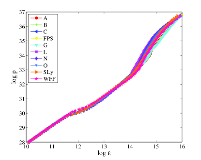
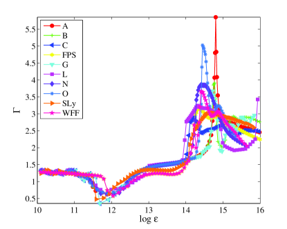
Figure 1: Pressure (top) and the adiabatic exponent (bottom) as a function of the total energy density for various EOS. Notice here we are using cgs units.

The composition of a neutron star consists qualitatively of three parts separated by transition points, see Fig. 1. At densities below the neutron drip, $\varepsilon<\varepsilon_{\rm d}\sim 10^{11}$ $\rm gcm^{-3}$ (the outer crust) the nuclei are immersed in an electron gas and the electron pressure is the principal contribute to the EOS. In the inner crust, $\varepsilon_{\rm d}<\varepsilon<10^{14}$ $\rm gcm^{-3}$, the gas is also composed of a fraction of neutrons unbounded from the nuclei and the EOS softens due to the attractive long-range behaviour of the strong interactions. For $\varepsilon>10^{14}$ $\rm gcm^{-3}$ a homogeneous plasma of nucleons, electrons, muons and other baryonic matter (e.g. hyperons), composes the core of the star. In this region the EOS stiffens because of the repulsive short-range character of the strong interactions. The bottom panel of Fig. 1 shows the adiabatic exponent which, under the assumption of thermodynamics equilibrium, determines the response of pressure to a local perturbation of density. We mention that, as explained in detail in Ref Douchin and Haensel (2001), in a pulsating NS the “actual adiabatic exponent” can be higher than that obtained from the EOS because the timescale of the beta processes are longer than the dynamical timescales of the pulsations. Thus the fraction of particles in a perturbed fluid element is assumed fixed to the unperturbed values (frozen composition). We refer the reader to Haensel et al. (2007) for all the details on neutron star structure and the complex physics behind it (e.g. elasticity of the crust, possible superfluid interior core, magnetic fields).

Table 2: Neutron Star models. From left to right the columns report: the name of the model, the EOS type, the mass $M$, the radius $R$, the compactness $M/R$, the central energy density $\varepsilon_{\rm c}$ and the central pressure $p_{c}$.

Model	EOS	$M$	$R$	$M/R$	$\varepsilon_{\rm c}$	$p_{\rm c}$
A10	A	1.00	6.55	0.15	1.96$\times 10^{-3}$	2.35$\times 10^{-4}$
A12	A	1.20	6.51	0.18	2.38$\times 10^{-3}$	3.76$\times 10^{-4}$
A14	A	1.40	6.39	0.22	3.01$\times 10^{-3}$	6.50$\times 10^{-4}$
A16	A	1.60	6.04	0.26	4.46$\times 10^{-3}$	1.49$\times 10^{-3}$
Amx	A	1.65	5.60	0.29	6.78$\times 10^{-3}$	3.24$\times 10^{-3}$
B10	B	1.00	5.78	0.17	1.37$\times 10^{-3}$	5.13$\times 10^{-4}$
B12	B	1.20	5.53	0.22	1.59$\times 10^{-3}$	1.02$\times 10^{-3}$
B14	B	1.40	4.96	0.28	1.88$\times 10^{-3}$	3.42$\times 10^{-3}$
Bmx	B	1.41	4.73	0.30	4.65$\times 10^{-3}$	5.33$\times 10^{-3}$
C10	C	1.00	8.15	0.12	3.35$\times 10^{-3}$	1.05$\times 10^{-4}$
C12	C	1.20	8.05	0.15	4.45$\times 10^{-3}$	1.67$\times 10^{-4}$
C14	C	1.40	7.90	0.18	7.76$\times 10^{-3}$	2.65$\times 10^{-4}$
C16	C	1.60	7.67	0.21	9.76$\times 10^{-3}$	4.49$\times 10^{-4}$
Cmx	C	1.85	6.69	0.28	1.18$\times 10^{-3}$	1.94$\times 10^{-3}$
FPS10	FPS	1.00	7.32	0.14	1.44$\times 10^{-3}$	1.50$\times 10^{-4}$
FPS12	FPS	1.20	7.30	0.16	1.75$\times 10^{-3}$	2.30$\times 10^{-4}$
FPS14	FPS	1.40	7.22	0.19	2.22$\times 10^{-3}$	3.64$\times 10^{-4}$
FPS16	FPS	1.60	7.02	0.23	4.77$\times 10^{-3}$	6.38$\times 10^{-4}$
FPSmx	FPS	1.80	6.22	0.29	1.45$\times 10^{-3}$	2.50$\times 10^{-3}$
G10	G	1.01	5.76	0.17	1.73$\times 10^{-3}$	5.36$\times 10^{-4}$
G12	G	1.20	5.42	0.22	2.10$\times 10^{-3}$	1.20$\times 10^{-3}$
Gmx	G	1.36	4.62	0.29	2.72$\times 10^{-3}$	5.65$\times 10^{-3}$
L10	L	1.00	9.61	0.10	5.55$\times 10^{-3}$	4.15$\times 10^{-5}$
L12	L	1.20	9.76	0.12	3.52$\times 10^{-3}$	5.60$\times 10^{-5}$
L14	L	1.40	9.89	0.14	5.03$\times 10^{-3}$	7.41$\times 10^{-5}$
L16	L	1.60	9.98	0.16	7.81$\times 10^{-4}$	9.75$\times 10^{-5}$
Lmx	L	2.68	9.23	0.29	5.80$\times 10^{-4}$	9.17$\times 10^{-4}$
N10	N	1.00	8.81	0.11	6.38$\times 10^{-4}$	5.70$\times 10^{-5}$
N12	N	1.20	8.98	0.13	7.05$\times 10^{-4}$	7.59$\times 10^{-5}$
N14	N	1.40	9.13	0.15	7.81$\times 10^{-4}$	9.97$\times 10^{-5}$
N16	N	1.60	9.24	0.17	2.33$\times 10^{-3}$	1.30$\times 10^{-4}$
Nmx	N	2.63	8.65	0.30	7.08$\times 10^{-4}$	1.20$\times 10^{-3}$
O10	O	1.00	8.29	0.12	1.41$\times 10^{-3}$	7.39$\times 10^{-5}$
O12	O	1.20	8.41	0.14	1.64$\times 10^{-3}$	1.03$\times 10^{-4}$
O14	O	1.40	8.50	0.16	1.96$\times 10^{-3}$	1.43$\times 10^{-4}$
O16	O	1.60	8.54	0.19	2.45$\times 10^{-3}$	1.97$\times 10^{-4}$
Omx	O	2.38	7.75	0.31	5.15$\times 10^{-3}$	1.66$\times 10^{-3}$
SLy10	SLy4	1.00	7.78	0.13	7.72$\times 10^{-4}$	1.12$\times 10^{-4}$
SLy12	SLy4	1.20	7.80	0.15	8.41$\times 10^{-4}$	1.66$\times 10^{-4}$
SLy14	SLy4	1.40	7.78	0.18	9.17$\times 10^{-4}$	2.45$\times 10^{-4}$
SLy16	SLy4	1.60	7.70	0.21	2.57$\times 10^{-3}$	3.70$\times 10^{-4}$
SLymx	SLy4	2.05	6.71	0.30	8.74$\times 10^{-4}$	2.50$\times 10^{-3}$
WFF10	WFF3	1.00	7.29	0.14	9.86$\times 10^{-4}$	1.46$\times 10^{-4}$
WFF12	WFF3	1.20	7.30	0.16	1.10$\times 10^{-3}$	2.18$\times 10^{-4}$
WFF14	WFF3	1.40	7.26	0.19	1.23$\times 10^{-3}$	3.34$\times 10^{-4}$
WFF16	WFF3	1.60	7.14	0.22	3.36$\times 10^{-3}$	5.48$\times 10^{-4}$
WFFmx	WFF3	1.84	6.40	0.29	1.18$\times 10^{-3}$	2.18$\times 10^{-3}$

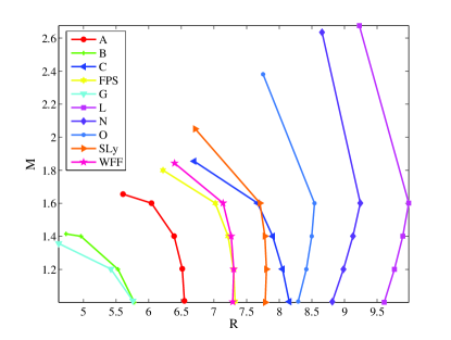
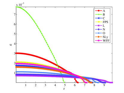
Figure 2: Top panel: mass versus radius for the NS models of Table 2. Bottom panel: profile of the total energy density $\varepsilon$ for all models with $M=1.4$.

Most of the mass (see the bottom panel of Fig. 2) is constituted by high density matter, so that the maximum mass of the star is essentially determined by the EOS of the core. On the other hand, the star radius strongly depends on the properties of the matter at low densities, due to Eq. (23).

To compensate the ignorance on the interior part of the star it is common to consider a large set of EOS derived from different models. In our work we employ 7 realistic EOS already used in Arnett and Bowers (1977), and in many other works (see for example Refs. Lindblom and Detweiler (1983); Andersson and Kokkotas (1998); Benhar et al. (2004); Kokkotas and Ruoff (2001); Benhar et al. (1999) on pulsations of relativistic stars, and Salgado et al. (1994); Stergioulas and Friedman (1995); Nozawa et al. (1998) on equilibrium models of rotating stars). Maintaining the same notation of Arnett and Bowers (1977), they are called A, B, C, G, L, N and O EOS. Most of the models in the sample are based on non-relativistic interactions modeled with Reid soft core type potentials. EOS N Walecka (1974) and O Bowers et al. (1975a, b) are instead based on relativistic interaction and many-body theories. Model G Canuto and Chitre (1974) is an extremely soft EOS, while L Arnett and Bowers (1977) is extremely stiff. EOS A Pandharipande (1971a) and C Bethe and Johnson (1974) are of intermediate stiffness. In addition, we use the FPS EOS Friedman and Pandharipande (1981); Lorenz et al. (1993), and the SLy EOS Douchin and Haensel (2001), modeled by Skyrme effective interactions. The FPS EOS, in particular is a modern version of Friedman and Pandharipande EOS Friedman and Pandharipande (1981). The last EOS considered is the UV14+TNI (here renamed WFF) EOS of Wiringa et al. (1988), which is an intermediate stiffness EOS based on two-body Urbana UV14 potential with the phenomenological three-nucleon TNI interaction. The composition is assumed to be of neutrons. For all the EOS models the inner crust is described by the BBS Baym et al. (1971a) or the HP94 Haensel and Pichon (1994) EOS, while for outer crust the BPS EOS Baym et al. (1971b) is used. We refer to Table 1 and cited references for further details.

Realistic EOS are usually given through tables. To use them in a numerical context it is necessary to interpolate between the tabulated values. The interpolation can not be chosen arbitrarily but must properly take into account the First Law of Thermodynamics, see e.g. Haensel and Proszynski (1982), that, in the case of a temperature independent EOS, reads:

$$p(n)=n^{2}\frac{d}{dn}\left(\frac{\varepsilon}{n}\right)$$ (25)

A thermodynamically consistent procedure is described in Swesty (1996) and it is based on Hermite poynomials. Essentially the method permits to interpolate a function forcing the match on the tabulated points both of the function and of its derivatives. We implement this scheme using cubic Hermite poynomials as already done in Nozawa et al. (1998), The procedure used is described in detail in Appendix A.

V Initial Data

In principle the choice of the initial data for the perturbation equations should take into account, at least approximately, the astrophysical scenario in which the neutron star is born. Such scenario could be, for example the gravitational collapse or the merger of two neutron stars. Only long-term simulations in full general relativity can investigate highly nonlinear and nonisotropic system until they settle down in a, almost spherical, quasi-equilibrium configuration. A perturbative analysis, like the one we propose, could then start from this point once the metric and matter tensors had been projected along the corresponding (tensorial) spherical harmonics. This approach, in principle possible, is however beyond the scopes of the present work.

Inspired by previous perturbative calculations Allen et al. (1998); Ruoff (2001), we consider different kinds of initial data such that they are the simplest, well-posed and involve perturbations of both the fluid and/or the metric quantities.

In the case of the even parity perturbations we start the evolutions from 3 different initial excitations of fluid and matter variables:

1. Conformally Flat Initial Data. We set $S(0,r)=0$ and give a fluid perturbation of type:

   $$H(0,r)=A\left(\frac{r}{R}\right)^{\ell-1}\sin\left(\pi(n+1)\frac{r}{R}\right).$$ (26)

   The function $k(0,r)$ is computed consistently solving the Hamiltonian constraint. The profile of $H$ in Eq. (26) is chosen in order to approximate the behavior of an enthalpy eigenfunction with $n$ nodes. In this way, only some modes can be (prominently) excited. Since we would like to focus on the principal fluid modes we chose a zero-nodes initial data setting $n=0$.

2. Radiative Initial Data. We set $k(0,r)=0$ and $H(0,r)$ as Eq. (26). The function $S(0,r)$ is computed consistently solving the Hamiltonian constraint.

3. Scattering-like Initial Data. We set $H(0,r)=0$ and $\Psi^{(\rm e)}(0,r)$ as a Gaussian pulse:

   $$\Psi^{(\rm e)}(0,r)=A\exp{\left(-\dfrac{(r-r_{\rm c})^{2}}{b^{2}}\right)},$$ (27)

   with $r_{\rm c}=70M$ and $b=M$. The functions $k(0,r)$ and $S(0,r)$ are computed consistently from Eqs. (11)-(II).

Initial data of type 1 and 2 are choosen to be time-symmetric ($S_{,t}=k_{,t}=H_{,t}=0$). On the one hand, this choice can be physically questionable because the system has an unspecified amount of incoming radiation in the past. On the other hand, it is the simplest choice and guaratees that the momentum constraints are trivially satisfied and only the Hamiltonian constraint needs to be used for the setup. The Gaussian in type 3 initial data is ingoing, i.e. $\Psi_{,t}=\Psi_{,r_{*}}$, and the derivatives of the other variables are computed consistently with this choice.

In the case of odd-parity perturbations we start the evolution using an ingoing narrow gaussian as in Eq. (27) for $\Psi^{(\rm o)}(0,r)$. The amplitude of the perturbation A is everywhere chosen equal to 0.01.

VI Results

For each EOS, we study a rapresentative set of models with $M=1$, $1.2$, $1.4$, $1.6$ and a model whose mass is close to the maximum mass allowed, for a total of 47 neutron stars. The principal equilibrium properties are summarized in Table 2. Fig. 2 shows the mass-radius diagram for all the models computed. The star radius spans a range from $R\sim 5$ (in the case of EOS B and G) to $R\sim 9-10$ (for EOS L and N). The order of stiffness of the EOS can be estimated, on average, as: G$<$B$<$A$<$FPS$<$WFF$<$SLy$<$C$<$O$<$N$<$L. For all the models described by a particular EOS, the compactness $M/R$ increases from about $0.1$ to $0.3$, corresponding to the increase of the star mass and the decrease of the radius. The (total) energy density profile as function of the radial coordinate in the bottom panel of Fig. 2 explains, as discussed above, that most of the mass is due to matter with density comparable to the central (maximum) density of the star.

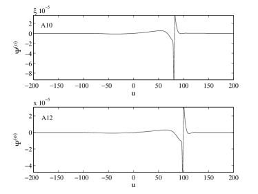
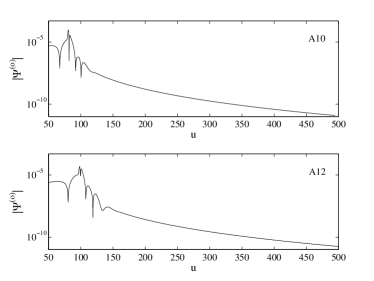
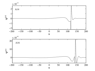
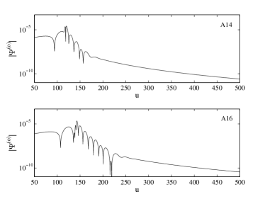
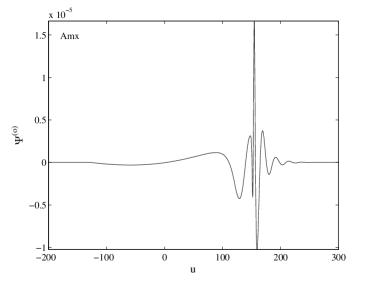
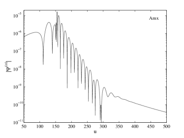
Figure 3: Excitation of $w$-modes in the odd parity waveforms, for different star models with EOS A, generated by the scattering of a Gaussian pulse of GWs with $b=M$. The mass and compactness of the star increases from top to bottom. The presence of $w$-modes is more evident for the more compact models. This qualitative behavior is common to all EOS.

For each model, we numerically evolve the equations for the odd and even-parity perturbations described in Sec. II using the initial data presented in Sec. V. All the details of the numerical schemes employed can be found in Appendix B. In the following sections we will discuss the results obtained focusing on the $\ell=2$ (quadrupole) multipole, as this is the principal responsible of the gravitational wave emission. The waves are extracted at different radii, $r^{\rm obs}=[50,\,100,\,200,\,300]M$. We checked the convergence of the waves and the differencies between the extraction at $r^{\rm obs}=200M$ and $r^{\rm obs}=300M$ are very small, so that we can infer to be sufficiently far away from the source. The gravitational waveforms we discuss in the following have always been extracted at the farthest observer, $r^{\rm obs}=300M$ and they are plotted versus observer’s retarded time $u=t-r^{\rm obs}_{*}$.

VI.1 Axial Waveforms

The gravitational waveform that results from scattering of Gaussian pulses of GWs off the odd-parity potential exhibits the well known structure (precursor-burst-ringdown-tail Davis et al. (1972)) analogue to the black holes case (see for example Ref. Bernuzzi et al. (2008) for the case of polytropic EOS). The characteristic signature of the star in the waveform is contained in the ringdown part, which is shaped by high frequencies, (quickly) exponentially damped oscillations: the $w$-modes Kokkotas and Schutz (1992). These modes are pure spacetime vibrations and are the analogue of black hole QNMs for relativistic stars Nollert (1999); Kokkotas and Schmidt (1999).

As a representative case, because the global qualitative features are common to all EOS, Fig. 3 exhibits waveforms computed only with EOS A. The compactness of the model increases from top to bottom; the left panels exhibit the waveforms on a linear scale, while the right panels their absolute values on a logarithmic scale. Since the damping time increases with the star compactness, the maximum mass model, Amx, presents the longest $w$-mode ringdown. On the contrary, model A10 exhibits only a one–cycle, small–amplitude ringdown oscillation that quickly disappears in the power-law tail.

In principle, an analysis of the frequency content of the axial waveforms by looking at the Fourier spectra or by means of a fit procedure based on a quasi-normal mode template is possible. Let us focus on model Amx, that presents the longest and clearest ringdown waveform. Using the same fit-analysis method of Bernuzzi et al. (2008) we estimate the frequency of the fundamental $w$-modes to be $\nu_{w}^{(\rm o)}=9452$ Hz, with a damping time $\tau_{w}^{(\rm o)}\simeq 0.07$ ms. For comparison, we note that a Schwarzschild black hole of the same mass has the fundamental $\ell=2$ frequency and damping time equal to, respectively, $\nu^{\rm BH}=7317$ Hz and $\tau^{\rm BH}=0.09$ ms. We have also computed the energy spectrum of the waveform starting from $u\sim 170$ (the first zero after the burst): the spectrum has a single peak centered at a frequency that differs from $\nu_{w}^{(\rm o)}$ of about a few percents. However, as discussed in Bernuzzi et al. (2008), we found that this information is in general very difficult to extract, especially for the lowest mass models, due to the rapid damping of the modes and their localization in a narrow time window. The comparison with frequency domain data (see Ref. Bernuzzi et al. (2008) for polytropic EOS and the discussion in Appendix B for realistic EOS) shows that the errors on the numbers presented above are of the order of 5%. The error on the frequencies increases up to about 12% for models with $M\sim 1.4$ and to about 20% for models with smaller mass. Moreover, the damping times can not be reliably estimated with a fit procedure when they are too short (see Table 3 in Appendix B). In summary, although the analysis of the waveforms through a fit procedure works for some particular models, in general it seems uncapable to give numbers as robust and reliable as those provided by a standard frequency domain approach. See for example Ref. Benhar et al. (1999) for details about this approach.

VI.2 Polar Waveforms

We start this section presenting together waveforms generated by conformally flat (type 1) and radiative (or non-conformally flat, type 2) initial data. Former studies with polytropic EOS Ruoff (2001); Nagar (2004) showed that initial data of type 1 determine the excitation of fluid modes only. On the contrary, initial data of type 2 produce a gravitational wave signal where both spacetime and fluid modes are present.

As expected, this qualitative picture is confirmed also for realistic EOS. Figure 4 exhibits the waveform $\Psi^{(\rm e)}$ for the representative model WFF14. For conformally flat initial data (solid line) the figure shows that the Zerilli-Moncrief function oscillates at (mainly) one frequency, of the order of the kHz. The corresponding energy spectrum (solid line in Fig. 5) reveals that the signal is in fact dominated by the frequency $\nu_{f}=2126$ Hz, but there is also a second peak at $\nu_{p}=6909$ Hz. This two frequencies are recognized as those of the fundamental fluid mode $f$ and of the first (pressure) $p$-mode.

For non-conformally flat initial data (dashed line in Fig. 4) the first part of the signal, i.e. $0\lesssim u\lesssim 50$, is dominated by a high-frequency and strongly-damped oscillation typical of curvature modes. For $u\gtrsim 50$, the type 1 and type 2 waveforms are practically superposed. The corresponding energy spectrum (dashed line in Fig. 5 has, superposed to the two narrow peaks of the fluid modes, a wide peak centered at higher frequency ($\sim 11$ kHz) that is typical of the presence of spacetime excitation Kokkotas and Schmidt (1999). 

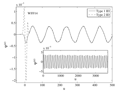
Figure 4: Even parity waveforms for model WFF14 generated by initial data of type 1 (solid line) and type 2 (dashed line). In the first case, only fluid modes (the $f$-mode and the first $p$-mode) are present; in the second case, $w$-mode oscillations are present at early times ($0\lesssim u\lesssim 50$). The inset shows long-term evolution (corresponding to a total time of $\sim 20$ ms) used to compute the energy spectrum of Fig. 5.

The information of Fig. 5 is complemented by the Fourier spectrum of the metric variable $S$ in Fig. 6. In contrast to the fluid variable $H$, which contains only narrow peaks for both kind of initial data, for type 2 waveforms the metric variable $S$ also exhibits a broad peak which is absent for type 1 initial data. Note, that the picture that we have discussed so far for model WFF14 remains qualitatively unchanged for all the other EOS.

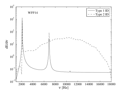
Figure 5: Energy spectra of the type 1 (solid line) and type 2 (dashed line) initial data evolution of Fig. 4. The two narrow peaks at 2126 Hz and 6909 Hz correspond to the $f$-mode and the first $p$-mode frequencies. The wide peak at $\simeq 11$ kHz corresponds to $w$-mode excitation.

Since our numerical scheme allows us to evolve the system in time as long as we wish, we can produce very long time-series to accurately extract, via Fourier analysis, the fluid mode frequencies. We did this analysis systematically for all the models considered. In Tables 4-5 in Appendix B we list the frequencies of the $f$-mode and the first $p$-mode extracted from the energy spectra. By comparison with the published frequencies of Andersson and Kokkotas Andersson and Kokkotas (1998) for some models with EOS A (obtained via frequency domain calculations), we estimate that the errors on our values are tipically smaller than 1%. For a fixed EOS, the frequencies increase with the star compactness. For a model of given mass, the $f$-mode frequency generally decreases if the EOS stiffens. The same (on average) is true for the first $p$-mode frequency. Following Ref. Andersson and Kokkotas (1998), we present in Fig. 7 the frequencies that we have computed as a function of the mean density $\sqrt{M/R^{3}}$ ($f$-mode) and of the compactness $M/R$ ($p$-mode) of the star. Globally, they show a very good quantitative agreement with previously published results calculated by means of a standard frequency domain approach Andersson and Kokkotas (1998).

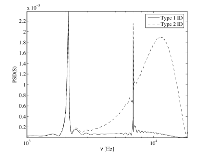
Figure 6: Power spectrum of the variable $S$ for model WFF14 in the case of initial data of type 1 and 2.

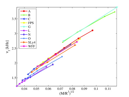
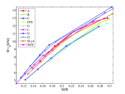
Figure 7: Comparison between the oscillation properties of models computed with different EOS. Top panel: $f$-mode frequencies as a function of $\sqrt{M/R^{3}}$. Bottom panel: the first $p$-mode frequency (multiplied by the mass $M$) as a function of the compactness $M/R$.

We conclude this section by discussing the waveforms generated by initial data of type 3. This kind of “scattering-type” initial condition constitutes the even-parity analogue of that discussed in Sec. VI.1 for the odd-parity case. In Fig. 8 we show the $\Psi^{(\rm e)}$ waveforms from 3 models of EOS WFF. The waveforms in the top panel of the figure are very similar to those of the left panels of Fig. 3. The logarithmic scale (bottom panel) highlights the main qualitative difference: i.e., fluid-mode oscillations are present, in place of the nonoscillatory tail, after the $w$-mode ringdown. Note that, in principle, the tail will emerge in the signal after that all the fluid modes have damped (i.e., on a time scale of a few seconds).

The process of $w$-mode excitation is instead exactly the same as for the odd parity case: the ringdown phase is longer (and thus clearly visible) for the more compact models. The frequencies are also very similar. For example, for model WFFmx (the one discussed in the figure) we have $\nu_{w}^{(\rm e)}=8638$ Hz and a damping time $\tau_{w}^{(\rm e)}\simeq 0.05$ ms, while for model Amx $\nu_{w}^{(\rm e)}=9798$ Hz and $\tau_{w}^{(\rm e)}\simeq 0.05$ ms (to be compared with $\nu_{w}^{(\rm o)}=9452$ and $\tau_{w}^{(\rm o)}\simeq 0.07$ ms).

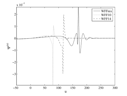
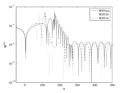
Figure 8: Excitation of even-parity $w$-modes for some WFF models from given initial data of type 3. As in the odd-parity case (compare with Fig. 3), the ringdown is more pronounced for more compact models.

VII Conclusions

In this work we have discussed the time-evolution of nonspherical (matter and gravitational) perturbations of nonrotating neutron stars described by a large sample of realistic EOS. The current study extends the work of Allen et al. Allen et al. (1998) and Ruoff Ruoff (2001), who focused essentially on polytropic, but one, EOS models. We have used an improved version of a recently developed 1D perturbative code Nagar et al. (2004) that has been thoroughly tested and used in the literature Nagar (2004); Nagar and Diaz (2004); Passamonti et al. (2007).

The main, new result, presented here is that our constrained numerical scheme allows us to stably evolve the even-parity perturbation equations without introducing any “special” coordinate change, as it was necessary in Ref. Ruoff (2001). In addition, despite the EOS that we consider are very different, the outcome of our computations is fully consistent (as expected) with previous studies involving polytropic EOS. In particular: (i) for even-parity perturbations, if the initial configuration involves a fluid excitation, (type 1 and 2 initial data), the Zerilli-Moncrief function presents oscillations at about 2-3 kHz due to the excitation of the fluid QNMs of the star; (ii) if we set $S\neq 0$ at $t=0$ (type 2, i.e. the non-conformally flat condition is imposed), high frequencies, strongly damped $w$-mode oscillations are always present in the waveforms; (iii) the $w$-mode excitation is generally weak, but it is less weak the more compact the star model is; consistently, (iv) for scattering-like initial data in both the odd and even-parity case the presence of $w$-modes is more striking the higher is the compactness of the star ; even-parity fluid modes are typically weakly excited in this case.

Thanks to the long-term and accurate evolutions we can perform, we extracted the fluid mode frequencies from the Fourier transform of time series of the waves with an accuracy comparable to that of frequency domain codes. For what concern the frequencies and damping times of spacetime modes, pretty good estimates can be obtained when damping times are not too short; i.e., for the more compact models. When these frequencies will be revealed in a gravitational wave signal, they will hopefully provide useful information on the internal structure of neutron stars. In particular, recognizing both fluid and $w$-modes in the signal could permit, in principle, to estimate the values of mass and radius of the NS and thus to put strong constraints on the EOS model Andersson and Kokkotas (1998); Benhar et al. (2004); Ferrari and Gualtieri (2008). We have limited our analysis to the first two fluid modes because they are the most responsible for gravitational waves emission. We checked that, by changing the initial fluid perturbation, our evolutionary description permits also to easily capture the frequencies of higher overtones Nagar and Diaz (2004).

In addition, despite all the approximation that we have introduced (initial data, no rotation, no magnetic fields), we believe that the approach to NS oscillations described in this paper can provide physical information complementary to that available from GR nonlinear evolutions. In particular, it can also be used to provide useful test-beds for GR nonlinear codes and must be seen as a first step to compare/constrast with nonlinear simulations of neutron star oscillations. In conclusion, since we can freely specify the initial data of the metric and matter variables at initial time, one can also think to use our present tool to evolve further in time an almost spherical configuration that is the outcome of a long-term numerical relativity simulation. A perturbative evolution like the one we discussed here (possibly complemented by a complex 3D (magneto)-hydrodynamics source, as an improvement of the approach discussed in Ref. Nagar et al. (2004)) could then start when the 3D fully nonlinear simulation ends.

Appendix A Table Interpolation

Here we describe the method used to interpolate the tables of the EOS. The interpolation scheme is based on Hermite polynomials and was introduced in Ref. Swesty (1996). We follow Nozawa et al. (1998) by using 3rd order (cubic) polynomials and we list here the relevant formulas for completeness. Consider a function $y(x)$, given the tables of $y_{j}$ and $y^{\prime}_{j}$ and a point $x_{\rm j}<x<x_{\rm j+1}$ the interpolated value $y(x)$ is:

$$y(x) =y_{i}H_{0}(w)+y_{i+1}H_{0}(1-w)$$ (28)

$$+\left(\frac{dy}{dx}\right)_{j}\Delta x_{j}H_{1}(w)$$

$$+\left(\frac{dy}{dx}\right)_{j+1}\Delta x_{j}H_{1}(1-w),$$

where

$$\Delta x_{j} \equiv(x_{j+1}-x_{j}),$$ (29)

$$w(x) \equiv\frac{x-x_{j}}{\Delta x_{j}}$$ (30)

and

$$H_{0}(w) =2w^{3}-3w^{2}+1,$$ (31)

$$H_{1}(w) =w^{3}-2w^{2}+w$$ (32)

are the cubic Hermite functions. The principal properties of this method are that for $x\rightarrow x_{j}$

$$y(x) \rightarrow y_{j},$$ (33)

$$y^{\prime}(x) \rightarrow y^{\prime}_{j}.$$ (34)

The EOS are usually given as 3 column tables with the values for $n$, $\varepsilon$ and $p$. In this work we need to compute $\varepsilon(p)$ and the speed of sound $C_{s}^{2}$. The thermodynamics consistency can be achived by computing, for a given value of $p$, first $n(p)$ and then $\varepsilon(n)$ imposing the derivative through Eq. (25). Finally the speed of sound is computed consistently with the interpolation. To obtain more accurate numerical data, we perform such calculations not directly on the functions, but taking logarithms. Violation of the first law of thermodynamics are typically less than 0.1%. We tested also other interpolation schemes, i.e. linear and spline interpolation, that in general gives violation of the thermodynamic principle of some percents.

As a check of the implementation, we evolved a polytropic model both with the analytic EOS and with tables of different numbers of entries. The results perfectly agree and we did not find any dependence on the tabulated points. In addition, the use of other interpolation schemes did not produce significant differences: this fact suggests that the global numerical errors of the code are dominant over the errors related to the violation of the thermodynamics principle. In the case of some tables (EOS FPS, SLy4 and L), we found that “high-order” interpolation (cubic Hermite and spline) did not permit an accurate reconstruction of the sound speed. This was due to spurious oscillations introduced by the high order derivatives. As a consequence, the code gave unphysical results. In all these cases, we adopted the linear interpolation.

Appendix B Numerical Details, code tests and mode frequencies

The code we employ in this work is a development of that described in Nagar (2004) and successfully used in many works Nagar and Diaz (2004); Nagar et al. (2004); Passamonti et al. (2006, 2007).

The TOV equations (21) are integrated numerically (from the center outward), for a given central pressure $p_{\rm c}$ (see Table 2), using a standard fourth-order Runge-Kutta integration scheme with adaptive step size.

To evolve numerically the perturbations equations, we introduce an evenly spaced grid in $r$ with uniform spacing $\Delta r$ and we adopt finite differencing approximation schemes for the derivatives. In particular, in the construction of the the computational grid the origin $r=0$ is excluded and the first point is located at $r=\Delta r/2$. The resolution is measured as the number of point $J_{i}$ inside the star radius. The star surface is located at a cell center $R=\Delta r/2+(J_{i}-1)\Delta r$.

The hyperbolic evolution equations for $S$ and $H$ are all solved with standard, second order convergent in time and space, leapfrog algorithm. For the evolution of the even-parity equations, the Hamiltonian constraint is used to update, at every time step, the variable $k$. This elliptic equation is discretized in space at second order and reduced to tridiagonal linear system that is inverted. For this reason the evolution scheme of the polar perturbations can be considered a constrained evolution. The inner boundary conditions of Eqs. (13)-(15) are implemented by setting to zero the variables at the first grid point. At the outer boundary, standard radiative Sommerfeld conditions are imposed.

The Zerilli-Moncrief function has been obtained in two (independent) ways. On the one hand, it has been computed from $S$ ($\chi$) and $k$ using Eq. (10) for every value of $r$. On the other hand, it has been computed using Eq. (10) only at the star surface ($r=R$, the matching point) and then evolved using Eq. (9). The second method has been used only as an independent consistency check and all the results discussed in this paper are obtained using the first method.

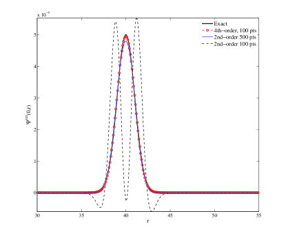
Figure 9: Convergence of the Zerilli function for initial data of type 3 for a polytropic EOS model. See text for discussion.

Table 3: Frequencies $\nu$ and damping times $\tau$ of fluid and spacetime modes of some models of Andersson and Kokkotas Andersson and Kokkotas (1998), described by EOS A, computed via our approach. The frequencies are expressed in Hz and the damping times in ms. For the sake of comparison, we report also the values of their Table A.1 with the “AK” superscript.

$M$	$\nu_{f}$	$\nu_{f}^{\rm AK}$	$\nu_{p}$	$\nu_{p}^{\rm AK}$	$\nu_{w}$	$\nu_{w}^{\rm AK}$	$\tau_{w}$	$\tau_{w}^{\rm AK}$
1.653	3080	3090	7825	7838	9342	9824	0.062	0.064
1.447	2580	2579	7843	7818	10038	11444	0.057	0.027
1.050	2183	2203	7555	7543	11267	14328	0.059	0.017

Table 4: Frequencies of the fluid modes for EOS A, B, C, FPS and G. From left to right the columns report: the name of the model, the EOS type, the $f$-mode frequency and the first $p$-mode frequency.

Model	EOS	$\nu_{f}$ [Hz]	$\nu_{p}$ [Hz]
A10	A	2146	7444
A12	A	2305	7816
A14	A	2512	7873
A16	A	2833	7823
Amx	A	3107	7848
B10	B	2705	7440
B12	B	3044	8061
B14	B	3577	8893
Bmx	B	3732	9091
C10	C	1617	5052
C12	C	1802	5349
C14	C	1933	5606
C16	C	2114	5876
Cmx	C	2627	6421
FPS10	FPS	1884	6326
FPS12	FPS	2028	6590
FPS14	FPS	2174	6764
FPS16	FPS	2325	6891
FPSmx	FPS	2820	7031
G10	G	2750	7510
G12	G	3097	8164
Gmx	G	3891	9080

Table 5: Frequencies of the fluid modes for EOS L, N, O, SLy and WFF. From left to right the columns report: the name of the model, the EOS type, the $f$-mode frequency and the first $p$-mode frequency.

Model	EOS	$\nu_{f}$ [Hz]	$\nu_{p}$ [Hz]
L10	L	1217	4599
L12	L	1297	4850
L14	L	1353	5025
L16	L	1395	5115
Lmx	L	1871	5109
N10	N	1415	5324
N12	N	1466	5694
N14	N	1497	5893
N16	N	1522	5960
Nmx	N	1952	5470
O10	N	1481	5924
O12	N	1578	6200
O14	N	1643	6283
O16	N	1734	6217
Omx	N	2217	5969
SLy10	SLy	1691	5818
SLy12	SLy	1804	6087
SLy14	SLy	1932	6279
SLy16	SLy	2029	6468
SLymx	SLy	2607	6601
WFF	WFF10	1889	6544
WFF	WFF12	1973	6766
WFF	WFF14	2126	6909
WFF	WFF16	2282	7016
WFF	WFFmx	2718	7016

In some situations, we found the convergence of the Zerilli-Moncrief computed from Eq. (10) particularly delicate. For example, in case of type 3 initial data (an even-parity Gaussian pulse of gravitational radiation) we realized that a very accurate computation of the radial derivative $k_{,r}$ is needed to obtain an accurate and reliable $\Psi^{(\rm e)}$ from $k$ and $S$. Fig. 9 summarizes the kind of problem that one can find computing the Zerilli-Moncrief function too naively. It refers to $\Psi^{(\rm e)}(r)$ at $t=0$. We consider (for simplicity of discussion) a polytropic model, i.e. $p=K\rho^{\Gamma}$ with $K=100$, $\Gamma=2$ and $\rho_{c}=1.28\times 10^{-3}$ with type 3 initial data (i.e. a Gaussian pulse with $\sigma=M$ centered at $r=40$). We fix $\Psi^{(\rm e)}$ by Eq. (27), we compute $\chi$ and $k$ from Eqs. (11)-(II), we compute $k_{,r}$ numerically and then we we reconstruct $\Psi^{(\rm e)}$ via Eq. (10). Fig. 9 shows that, for low resolution ($J_{i}=100$), using a second-order finite-differencing standard stencil to compute $k_{,r}$ is clearly not enough, as the reconstructed (thicker dashed-dot line) and the “exact” (solid line) $\Psi^{(\rm e)}$ are very different. Incrasing the resolution (to 500 points) improves the agreement, which is however not perfect yet (thinner dashed-dot line). A visible improvement is obtained using higher order finite-differencing operators: the figure shows that a 4th-order operator (already in the low-resolution case with $J_{i}=100$ points) is sufficient to have an accurate reconstruction of the Zerilli-Moncrief function. The conclusion is that one needs to use at least 4th-order finite-differencing operators to compute accurately $\Psi^{(\rm e)}$ from $\chi$ and $k$. If this is not done, the resulting function is not reliable and it can’t be considered a solution of Eq. (9). Typically, we have seen that, when this kind of inaccuracy is present, the amplitude of (part of) the Zerilli-Moncrief function (usually the one related to the $w$-mode burst) grows linearly with $r$ instead of tending to a constant value for $r\to\infty$.

We performed extensive simulations to test the code. The scheme is stable and permits us to accurately evolve the equations as long as we wish. To check convergence of the waves, we run different resolutions and we computed the energy emitted at infinity (last detector) integrating separately the ${\ell}=2$ odd and even contribute of Eq. (19) over the evolution time interval. The value of the energy converges correctly up to second order terms, $\mathcal{O}(\Delta r^{2})$.

To validate the physical results of the code we compare the frequencies extracted from our simulations with values computed via a frequency domain approach. In the case of the polytropic EOS, the results reported in Ref. Nagar and Diaz (2004) showed that the errors on fluid frequencies are less than 1%. Spacetime frequencies for polytropic EOS models were checked in Ref. Bernuzzi et al. (2008). In this case, when the damping times are sufficiently long (i.e. when a narrow Gaussian pulse is used and the star model is very compact), it is possibile to estimate $\nu$ and $\tau$ using a fit procedure, with an error of the order of 6%.

The accuracy of the frequencies does not change when we use realistic EOS. To validate this assertion, we compared the frequencies extracted from our waveforms with those of Andersson and Kokkotas Andersson and Kokkotas (1998) for EOS A with mass $M=1.653$, $M=1.447$ and $M=1.050$ (see Table A.1 of Ref. Andersson and Kokkotas (1998)). Our results are listed in Table 3, together with the data of Andersson and Kokkotas (1998) for completeness. Fluid frequencies are typically captured with an accuracy below 1%, while spacetime frequencies and damping times can be estimate with decent accuracy (5%) only for the maximum mass model. As a consequence, we expect that a similar accuracy for fluid modes, i.e. of the order of 1%, should be expected for the 47 NS models of Table 2. For completeness, the corresponding frequencies are listed in Table 4 and Table 5.

The simulations we have discussed in the main text of the paper use resolutions of $J_{i}=400$ and $J_{i}=800$ respectively for the odd and even-parity case. The Courant-Friedrichs-Lewy factor is set to $\Delta t/\Delta r=0.4$. For each model, the outer boundary of the grid is at $r=600M$. The final evolution time is $t^{\rm end}=3000M$ for even-parity evolutions and $t^{\rm end}=800M$ for the odd-parity ones.

References

- Shapiro and Teukolsky (1983) S. L. Shapiro and S. A. Teukolsky, Black holes, white dwarfs, and neutron stars: The physics of compact objects (Wiley, New York, USA, 1983).
- Kokkotas and Schmidt (1999) K. D. Kokkotas and B. Schmidt, Living Reviews in Relativity 2 (1999), URL http://www.livingreviews.org/lrr-1999-2.
- Kokkotas and Ruoff (2002) K. D. Kokkotas and J. Ruoff (2002), eprint gr-qc/0212105.
- Andersson and Kokkotas (1998) N. Andersson and K. D. Kokkotas, Mon. Not. Roy. Astron. Soc. 299, 1059 (1998), eprint gr-qc/9711088.
- Baiotti et al. (2005) L. Baiotti et al., Phys. Rev. D71, 024035 (2005), eprint gr-qc/0403029.
- Shibata et al. (2006) M. Shibata, Y. T. Liu, S. L. Shapiro, and B. C. Stephens, Phys. Rev. D 74, 104026 (2006).
- Shibata et al. (2005) M. Shibata, K. Taniguchi, and K. Uryū, Phys. Rev. D 71, 084021 (2005).
- Dimmelmeier et al. (2007) H. Dimmelmeier, C. D. Ott, H.-T. Janka, A. Marek, and E. Muller, Phys. Rev. Lett. 98, 251101 (2007).
- Dimmelmeier et al. (2006) H. Dimmelmeier, N. Stergioulas, and J. A. Font, Mon. Not. Roy. Astron. Soc. 368, 1609 (2006), eprint astro-ph/0511394.
- Kokkotas and Ruoff (2001) K. D. Kokkotas and J. Ruoff, Astron. Astrophys. 366, 565 (2001), eprint gr-qc/0011093.
- Allen et al. (1998) G. Allen, N. Andersson, K. D. Kokkotas, and B. F. Schutz, Phys. Rev. D58, 124012 (1998), eprint gr-qc/9704023.
- Ruoff (2001) J. Ruoff, Phys. Rev. D63, 064018 (2001).
- Nagar et al. (2004) A. Nagar, G. Diaz, J. A. Pons, and J. A. Font, Phys. Rev. D69, 124028 (2004), eprint gr-qc/0403077.
- Andersson and Kokkotas (1996) N. Andersson and K. D. Kokkotas, Phys. Rev. Lett. 77, 4134 (1996), eprint gr-qc/9610035.
- Nagar and Diaz (2004) A. Nagar and G. Diaz, in Proceedings of 27th Spanish Relativity Meeting (ERE 2003): Gravitational Radiation, Alicante, Spain, 11-13 Sep 2003 (2004), eprint gr-qc/0408041.
- Passamonti et al. (2007) A. Passamonti, N. Stergioulas, and A. Nagar, Phys. Rev. D75, 084038 (2007), eprint gr-qc/0702099.
- Passamonti et al. (2006) A. Passamonti, M. Bruni, L. Gualtieri, A. Nagar, and C. F. Sopuerta, Phys. Rev. D73, 084010 (2006), eprint gr-qc/0601001.
- Ferrari and Kokkotas (2000) V. Ferrari and K. D. Kokkotas, Phys. Rev. D62, 107504 (2000), eprint gr-qc/0008057.
- Ruoff et al. (2001) J. Ruoff, P. Laguna, and J. Pullin, Phys. Rev. D63, 064019 (2001), eprint gr-qc/0005002.
- Ferrari et al. (2004a) V. Ferrari, L. Gualtieri, J. A. Pons, and A. Stavridis, Mon. Not. Roy. Astron. Soc. 350, 763 (2004a), eprint astro-ph/0310896.
- Ferrari et al. (2004b) V. Ferrari, L. Gualtieri, J. A. Pons, and A. Stavridis, Class. Quant. Grav. 21, S515 (2004b), eprint astro-ph/0409578.
- Stavridis and Kokkotas (2005) A. Stavridis and K. D. Kokkotas, Int. J. Mod. Phys. D14, 543 (2005), eprint gr-qc/0411019.
- Nagar (2004) A. Nagar, PhD Thesis, University of Parma (unpublished) (2004).
- Charles W. Misner and Wheeler (1973) K. S. T. Charles W. Misner and J. A. Wheeler, Gravitation (W. H. Freeman and Company, San Francisco, 1973).
- Gerlach and Sengupta (1979) U. H. Gerlach and U. K. Sengupta, Phys. Rev. D19, 2268 (1979).
- Gerlach and Sengupta (1980) U. H. Gerlach and U. K. Sengupta, Phys. Rev. D22, 1300 (1980).
- Gundlach and Martin-Garcia (2000) C. Gundlach and J. M. Martin-Garcia, Phys. Rev. D61, 084024 (2000), eprint gr-qc/9906068.
- Martin-Garcia and Gundlach (2001) J. M. Martin-Garcia and C. Gundlach, Phys. Rev. D64, 024012 (2001), eprint gr-qc/0012056.
- Regge and Wheeler (1957) T. Regge and J. A. Wheeler, Phys. Rev. 108, 1063 (1957).
- Zerilli (1970) F. J. Zerilli, Phys. Rev. Lett. 24, 737 (1970).
- Moncrief (1974) V. Moncrief, Ann. Phys. 88, 323 (1974).
- Nagar and Rezzolla (2005) A. Nagar and L. Rezzolla, Class. Quant. Grav. 22, R167 (2005), eprint gr-qc/0502064.
- Chandrasekhar and Ferrari (1991) S. Chandrasekhar and V. Ferrari, Proc. Roy. Soc. Lond. A432, 247 (1991).
- Martel and Poisson (2005) K. Martel and E. Poisson, Phys. Rev. D71, 104003 (2005), eprint gr-qc/0502028.
- Pandharipande (1971a) V. R. Pandharipande, Nucl. Phys. A174, 641 (1971a).
- Pandharipande (1971b) V. R. Pandharipande, Nucl. Phys. A178, 123 (1971b).
- Bethe and Johnson (1974) H. A. Bethe and M. B. Johnson, Nucl. Phys. A230, 1 (1974).
- Lorenz et al. (1993) C. P. Lorenz, D. G. Ravenhall, and C. J. Pethick, Physical Review Letters 70, 379 (1993).
- Friedman and Pandharipande (1981) B. Friedman and V. R. Pandharipande, Nuclear Physics A 361, 502 (1981).
- Canuto and Chitre (1974) V. Canuto and S. M. Chitre, Phys. Rev. D 9, 1587 (1974).
- Arnett and Bowers (1977) W. D. Arnett and R. L. Bowers, Astrophys.J.Suppl.Series 33, 415 (1977).
- Walecka (1974) J. D. Walecka, Annals of Physics 83, 491 (1974).
- Bowers et al. (1975a) R. L. Bowers, A. M. Gleeson, and R. Daryl Pedigo, Phys. Rev. D 12, 3043 (1975a).
- Bowers et al. (1975b) R. L. Bowers, A. M. Gleeson, and R. Daryl Pedigo, Phys. Rev. D 12, 3056 (1975b).
- Douchin and Haensel (2001) F. Douchin and P. Haensel, Astron. Astrophys. 380, 151 (2001), eprint astro-ph/0111092.
- Wiringa et al. (1988) R. B. Wiringa, V. Fiks, and A. Fabrocini, Phys. Rev. C38, 1010 (1988).
- Haensel et al. (2007) P. Haensel, A. Y. Potekhin, and D. G. Yakovlev, Neutron stars 1: Equation of state and structure (Springer, New York, USA, 2007).
- Benhar et al. (2004) O. Benhar, V. Ferrari, and L. Gualtieri, Phys. Rev. D70, 124015 (2004), eprint astro-ph/0407529.
- Benhar et al. (1999) O. Benhar, E. Berti, and V. Ferrari, Mon. Not. Roy. Astron. Soc. 310, 797 (1999), eprint gr-qc/9901037.
- Lindblom and Detweiler (1983) L. Lindblom and S. L. Detweiler, Astrophys. J. Suppl. Ser. 53, 73 (1983).
- Nozawa et al. (1998) T. Nozawa, N. Stergioulas, E. Gourgoulhon, and Y. Eriguchi, Astron. Astrophys. Suppl. Ser. 132, 431 (1998), eprint gr-qc/9804048.
- Salgado et al. (1994) M. Salgado, S. Bonazzola, E. Gourgoulhon, and P. Haensel, Astron. Astrophys. 291, 155 (1994).
- Stergioulas and Friedman (1995) N. Stergioulas and J. L. Friedman, Astrophys. J. 444, 306 (1995), eprint astro-ph/9411032.
- Baym et al. (1971a) G. Baym, H. A. Bethe, and C. J. Pethick, Nuclear Physics A 175, 225 (1971a).
- Haensel and Pichon (1994) P. Haensel and B. Pichon, Astron. Astrophys. 283, 313 (1994), eprint nucl-th/9310003.
- Baym et al. (1971b) G. Baym, C. Pethick, and P. Sutherland, Astrophys. J. 170, 299 (1971b).
- Haensel and Proszynski (1982) P. Haensel and M. Proszynski, Astrophys. J. 258, 306 (1982).
- Swesty (1996) F. D. Swesty, J.Comput.Phys. 127, 118 (1996), ISSN 0021-9991.
- Davis et al. (1972) M. Davis, R. Ruffini, and J. Tiomno, Phys. Rev. D5, 2932 (1972).
- Bernuzzi et al. (2008) S. Bernuzzi, A. Nagar, and R. De Pietri, Phys. Rev. D77, 044042 (2008), eprint arXiv:0801.2090 [gr-qc].
- Kokkotas and Schutz (1992) K. D. Kokkotas and B. F. Schutz, Mon. Not. Roy. Astron. Soc. 225, 119 (1992).
- Nollert (1999) H.-P. Nollert, Class. and Q. Grav. 16, 159 (1999).
- Ferrari and Gualtieri (2008) V. Ferrari and L. Gualtieri, Gen. Rel. Grav. 40, 945 (2008), eprint 0709.0657.
- Stergioulas and Morsink (Web Resource) N. Stergioulas and S. Morsink, UWM Centre for Gravitation and Cosmlogy (Web Resource), URL http://www.gravity.phys.uwm.edu/rns/.
- Haensel and Potekhin (Web Resource) P. Haensel and A. Y. Potekhin, Neutron Star Group, Ioffe Institute (Web Resource), URL http://www.ioffe.ru/astro/NSG/NSEOS/.
- Haensel and Potekhin (2004) P. Haensel and A. Y. Potekhin, Astron. Astrophys. 428, 191 (2004), eprint astro-ph/0408324.