The electron transport through a quantum dot in the Coulomb blockade regime: Non-equilibrium Green’s functions based model

Abstract

We explore electron transport through a quantum dot coupled to the source and drain charge reservoirs. We trace the transition from the Coulomb blockade regime to Kondo regime in the electron transport through the dot occuring when we gradually strengthen the coupling of the dot to the charge reservoirs. The current-voltage $(I-V)$ characteristics are calculated using the equations of motion approach within the nonequilibrium Green’s functions formalism (NEGF) beyond the Hartree-Fock approximation. We show that within the Coulomb blockade regime the $I-V$ characteristics for the quantum dot containing a single spin-degenerated level with the energy $E_{0}$ include two steps whose locations are determined by the values of $E_{0}$ and the energy of Coulomb interaction of electrons in the dot $U.$ The heights of the steps are related as $2:1$ which is consistent with the results obtained by means of the transition rate equations.

I i. Introduction:

As known, quantum dots host such interesting quantum transport phenomena as Coulomb blockade 1 and Kondo effect 2 ; 3 . Fast development of experimental technique in recent years provides broad opportunities for fabrication of devices including novel active elements such as single molecules, nanowires and carbon nanotubes, placed in between metallic leads. Such junctions are commonly treated as quantum dots coupled to the macroscopic charge reservoirs which play the parts of source and drain in the electron transport. Current achievements in nanoelectronics make it possible to observe electron transport through realistic junctions varying external parameters (source-drain and gate voltage and temperature) and internal characteristics of the junction, e.g. the coupling strength of the quantum dot to the source and drain reservoirs. As a result, both supression of the electron transport through the quantum dot at small values of the source-drain voltage $(V)$ arising due to the high charging energy inside the dot (Coulomb blockade), and the increase in the electrical conduction of the junction at $V\approx 0$ due to the Kondo effect were repeatedly observed in experiments on molecular and carbon nanotubes junctions 4 ; 5 ; 6 ; 7 ; 8 ; 9 ; 10 ; 11 ; 12 ; 13 ; 14 .

The Coulomb blockade occurs when the quantum dot representing a molecule or a carbon nanotube is weakly coupled to the source and drain which means that the charging energies $U$ are much greater than the contact and temperature induced broadening of the electron levels in the dot. Theoretical studies of the electron transport through a quantum dot within the Coulomb blockade regime mostly employ “master” equations for the transition rates between the states of the dot differing by a single electron 15 ; 16 ; 17 ; 18 . It was shown that the current-voltage curves for a dot including a single spin-degenerated level exhibite two steps. The steps correspond to the gradual adding/removing two electrons with the different spin orientations to/from the dot. Assuming the symmetric contacts of the dot with both charge reservoirs, the first step in the current-voltage curve must be two times higher than the second one (see Refs. 18 ; 19 ). This result has a clear physical sense. Obviously, one may put the first electron of an arbitrary spin orientation to the empty level in the dot. However, the spin of the second electron added to the dot is already determined by the spin of the first one. So, there are two ways to add/remove the first electron to/from the empty/filled level in the dot but only one way to add/remove the second one.

While the approach based on the transition rates “master” equations brings sound results within the Coloumb blockade regime, its generalization to the case of stronger coupled junctions is not justified. More sophisticated methods employing various modifications of the nonequilibrium Green’s functions formalism (NEGF) are developed to analyze electron transport through quantum dots coupled to the leads 20 . These theoretical techniques were repeatedly employed to calculate the retarded/advanced and lesser Green’s functions for the dot. The Green’s functions are needed to compute the electron density of states (DOS) on the dot where the Kondo peak could be manifested, as well as the electron current through the junction. A commonly used approach within the NEGF is the equations of motion (EOM) method which was first proposed to describe quantum dot systems by Meir, Wingreen and Lee 21 . This technique enables to express the relevant Green’s functions in terms of higher-order Green’s functions. Writing out EOM for the latter, one arrives at the infinite sequence of the equations successively involving Green’s functions of higher orders.

To get expressions for the necessary Green’s functions this system of EOM must be truncated. Also, higher-order Green’s functions still included in the remaining EOM must be approximated to express them by means of the lower-order Green’s functions. In outline, this procedure is well-known and commonly used. However, in numerous existing papers important details of the above procedure vary which brings different approximations for the relevant Green’s functions. Accordingly, the results of theoretical studies of the quantum dot response vary.

The NEGF formalism was successfully applied to describe the quantum dot response within the Coulomb blockade regime (weak coupling of the dot to the electron reservoirs), using the expressions for both retarded and lesser Green’s function within the Hartree-Fock approximation 22 ; 23 . The results for the electron transport through the quantum dot obtained in these works give the correct ratio of the subsequent current steps, namely: $2:1,$ assuming the dot to be symmetrically coupled to the leads. It is a common knowledge that within the Hartree-Fock approximation one cannot catch the Kondo peak. To quantitatively describe this effect one may need to include hybridization up to very high orders in calculation of the lead-dot coupling parameters, and the studies aiming at better theoretical analysis of the Kondo effect started by Meir et al 24 are still in progress (see. e.g. Refs. 20 ; 25 ; 26 ).

Obviously, the Green’s functions suitable to reveal the Kondo peak in the electron DOS on the dot must provide the proper description of the transport through the dot within the Coulomb blockade regime when leads-dot couplings are weak. However, usually NEGF based results beyond the Hartree-Fock approximation successfully employed to describe the Kondo effect and related phenomena, were not applied to the limiting case of the Coulomb blockade. In those works were such application was carried out, the correct ratio of heights of the subsequent current steps, namely $2:1,$ was not obtained. For instance, Muralidharan, Ghosh and Datta 18 reported the results on NEGF calculations which give equal heights of the two steps on the current-voltage curve within the Coulomb blockade regime, and Galperin, Nitzan and Ratner studies 20 result in the heights ratio about $1.6:1.$ So, up to present there exists a discrepancy between NEGF and master equations based results. This discrepancy may not be easily disregarded for its existence makes questionable general and useful results based on the advanced techniques within the NEGF formalism. Recently, the above disagreement was discussed in the Ref. 18 .

The purpose of the present work is to clarify the issue, and to erase the above disconsistency. We apply equation of motion based approach to NEGF method to get a description of both Coulomb blockade and Kondo regimes in the electron transport through a quantum dot within the same computational procedure for the relevant Green’s functions. We show that the assumed approximations give correct ratio of heights of the steps in the current-voltage curves within the Coulomb blockade limit and allow to get the Kondo peak, as well. For simplicity, we omit from consideration dissipative effects, and we concentrate on a non-magnetic quantum dot coupled to non-ferromagnetic leads. Obtained results are valid for an arbitrary value of the Coulomb interaction on the dot, assuming that the latter is stronger than dot-leads coupling. Also, the analysis may be generalized to magnetic systems and to dots containing many levels provided that the charging energy is small compared to the adjacent levels separations. We remark that the present analysis is confined with using simplest possible approximations for the necessary Green’s functions. Therefore we do not take into account corrections proposed in Ref. 26 to better approximate the Kondo peak.

II ii. Main equations

We write the Hamiltonian of the junction including the dot and source and drain reservoirs (leads) as:

$$H=H_{L}+H_{R}+H_{D}+H_{T}.$$ (1)

Here, the terms $H_{\beta}\ (\beta=L,R)$ corrrespond to the left and right leads and describe them within the noninteracting particles approximation

$$H_{\beta}=\sum_{r\sigma}\epsilon_{r\beta\sigma}c_{r\beta\sigma}^{+}c_{r\beta\sigma}$$ (2)

where $\epsilon_{r\beta\sigma}$ are the single-electron energies in the electrode $\beta$ for the electron states $r,\sigma$ (the index $\sigma$ labeling spin up and spin down electrons), and $c_{r\beta\sigma}^{+},c_{r\beta\sigma}$ denote the creation and annihilation operators for the electrodes. We assume that energy levels $\epsilon_{r\beta\sigma}$ in the electron reservoirs are uniformly spaced over the ranges corresponding to the electron conduction bands for both spin orientations. The spacing between two adjacent levels $\delta\epsilon_{\beta\sigma}$ is supposed to be much smaller than the bandwidth $\Delta_{\beta\sigma}\ (\delta\epsilon_{\beta\sigma}/\Delta_{\beta\sigma}\sim 10^{-4}).$

The term $H_{D}$ describes the dot itself. Taking into account the electron-electron interaction, this term has the form:

$$H_{D}=\sum_{\sigma}E_{\sigma}c^{+}_{\sigma}c_{\sigma}+Uc_{\uparrow}^{+}c_{\uparrow}c_{\downarrow}^{+}c_{\downarrow}$$ (3)

where $c_{\sigma}^{+},c_{\sigma}$ are the creation and annihilation operators for the electrons in the dot; $E_{\sigma}=E_{0}$ is the energy of the single dot level, the energy $U$ characterizes the Coulomb interaction of electrons in the dot. We carry out calculations within the low temperature regime, so $U$ is supposed to significantly exceed the thermal energy $kT.$ The last term in the Hamiltonian Eq. 1 describes the coupling of the reservoirs to the dot:

$$H_{T}=\sum_{r\beta\sigma}\tau_{r\beta\sigma}^{*}c_{r\beta\sigma}^{+}c_{\sigma}+H.c.$$ (4)

where $\tau_{r\beta\sigma}$ are the coupling parameters describing the coupling of the $r,\sigma$ electron states belonging to the electrode $\beta$ to the quantum dot.

Now, we employ the equations of motion method to compute the retarded Green’s function for the dot. Since no spin-flip processes on the dot are taken into account, and we assume the electron transport to be spin-conserving, we may separately introduce the Green’s functions for each spin channel. The computational procedure is described in the Appendix. We obtain:

$$G_{\sigma}^{rr}(E)=\frac{E-E_{0}-\Sigma_{02}^{\sigma}-U(1-\big{<}n_{-\sigma}\big{>})}{(E-E_{0}-\Sigma_{0\sigma})(E-E_{0}-U-\Sigma_{02}^{\sigma})+U\Sigma_{1\sigma}},$$ (5)

Here, $\big{<}n_{-\sigma}\big{>}=\big{<}c_{-\sigma}^{+}c_{-\sigma}\big{>},$ and self energy corrections are given by:

$$\Sigma_{0\sigma}= \sum_{r\beta}\frac{|\tau_{r\beta\sigma}|^{2}}{E-\epsilon_{r\beta\sigma}+i\eta},$$ (6)

$$\Sigma_{1\sigma}= \sum_{r\beta}|\tau_{r\beta,-\sigma}|^{2}f_{r,-\sigma}^{\beta}\left\{\frac{1}{E-2E_{0}-U+\epsilon_{r\beta,-\sigma}+i\eta}\right.$$

$$+\left.\frac{1}{E-\epsilon_{r\beta,-\sigma}+i\eta}\right\},$$ (7)

$$\Sigma_{2\sigma}= \sum_{r\beta}|\tau_{r\beta,-\sigma}|^{2}\left\{\frac{1}{E-2E_{0}-U+\epsilon_{r\beta,-\sigma}+i\eta}\right.$$

$$+\left.\frac{1}{E-\epsilon_{r\beta,-\sigma}+i\eta}\right\},$$ (8)

$$\Sigma_{02}^{\sigma}= \Sigma_{0\sigma}+\Sigma_{2\sigma}.$$ (9)

Here, $f_{r\sigma}^{\beta}$ is the Fermi distribution function for the energy $\epsilon_{r\beta\sigma}$ and the chemical potential $\mu^{\beta}$ and $\eta$ is a positive infinitesimal parameter. The expression 5 for the Green’s function $G_{\sigma}^{rr}(E)$ was first derived by Meir and Wingreen 21 . Later, the same expression was obtained in Ref. 25 and (assuming that the electron energy levels on the leads are spin degenerate) in the book 19 . It was repeatedly used to qualitatively describe the Kondo peak in the electron DOS (see e.g. Refs. 24 ; 25 ). As shown in these works, the Kondo peak originates from the last term in the denominator of the Eq. 5. At low temperatures the real part of the self-energy term $\Sigma_{1\sigma}$ diverges giving rise to the peak at $\mu^{L}=\mu^{R}=E.$ Better approximations for the Green’s function $G_{\sigma}^{rr}(E)$ such as that derived in the Ref. 26 may give better results for the shape and height of the Kondo peak. However, the very emergence of the latter is accounted for in the Eq. 5.

The occupation numbers $\big{<}n_{\sigma}\big{>}=\big{<}c_{\sigma}^{+}c_{\sigma}\big{>}$ and $\big{<}n_{-\sigma}\big{>}=\big{<}c_{-\sigma}^{+}c_{-\sigma}\big{>}$ may be found solving the integral equations of the form:

$$\big{<}n_{\sigma}\big{>}=\frac{1}{2\pi}\int dE\mbox{Im}(G_{\sigma}^{<})$$ (10)

where the lesser Green’s fucntion $G_{\sigma}^{<}$ is introduced. The function $G_{\sigma}^{<}$ obeys the Keldysh equation:

$$G_{\sigma}^{<}(E)=G_{\sigma}^{rr}(E)\Sigma_{\sigma}^{<}G_{\sigma}^{aa}(E)$$ (11)

where $G_{\sigma}^{aa}(E)$ is the Fourier component of the advanced Green’s function. The Fourier transform of the lesser Green’s function $G_{\sigma}^{<}$ is related to the Fourier transforms of the retarded and advanced Green’s functions of the form 5, so the quantities $\big{<}n_{\sigma}\big{>}$ and $\big{<}n_{-\sigma}\big{>}$ appear in the integrands in the right hand sides of the equations 10 for both spin directions. In further calculations we use the following expression for $\Sigma_{\sigma}^{<}:$

$$\Sigma_{\sigma}^{<}=i\sum_{\beta}f_{\sigma}^{\beta}(E)\Gamma_{\sigma}^{\beta}.$$ (12)

Consequently, we have

$$G_{\sigma}^{<}=iG_{\sigma}^{rr}(E)G_{\sigma}^{aa}(E)\left[\Gamma_{\sigma}^{L}f^{L}_{\sigma}(E)+\Gamma_{\sigma}^{R}f^{R}_{\sigma}(E)\right]$$ (13)

where $f^{L,R}_{\sigma}(E)$ are the Fermi distribution functions for the left/right reservoirs, and

$$\Gamma_{\sigma}^{\beta}=-2\mbox{Im}\left(\Sigma_{0\sigma}^{\beta}\right)$$ (14)

where

$$\Sigma_{0\sigma}^{\beta}=\sum\limits_{r}\displaystyle\frac{|\tau_{r\beta\sigma}|^{2}}{E-\epsilon_{r\beta\sigma}+i\eta}.$$ (15)

Employing the expression 12 for $\Sigma_{\sigma}^{<}$ we assume that the Coulomb interaction of the electrons on the dot does not affect the coupling of the latter to the leads, as well as it occurs within the Hartree-Fock approximation 22 . Such assumption agrees with the way of estimating averages in the process of decoupling of high-order Green’s functions which was used to derive Eq. 5. It seems reasonable while the dot coupling to the leads is weaker than the characteristic energy of the Coulomb interactions on the dot. The proper choice of approximation for the lesser Green’s function is very important for it directly affects the values of occupation numbers $\big{<}n_{\pm\sigma}\big{>}$ and, consequently, the heights of the peaks in the electron DOS in the Coulomb blockade regime. Also, the relative heights of the steps in the current-voltage characteristics depend on the occupation numbers. The employed form for $G_{\sigma}^{<}(E)$ differs form those used in some previous works (see e.g. Refs. 20 ; 25 ) where extra terms arising due to the Coulomb interaction on the dot are inserted in the expression for $\Sigma_{\sigma}^{<}.$ Certainly, one may expect such terms to appear as corrections to the main approximation 12. However, these terms must become insignificant and negligible in the Coulomb blockade regime when the dot is weakly coupled to the leads. The expression for $\Sigma_{\sigma}^{<}$ reported in Ref. 25 does not satisfy this requirement.

Substituting Eq. 5 into Eq. 13 and inserting the result into Eq. 10 we obtain the system of equations to find the mean occupation numbers of electrons on the dot:

$$\big{<}n_{\pm\sigma}\big{>}=P_{\pm\sigma}+U\big{<}n_{\mp\sigma}\big{>}Q_{\pm\sigma}+U^{2}\big{<}n_{\mp\sigma}\big{>}^{2}R_{\pm\sigma}.$$ (16)

Here,

$$P_{\pm\sigma}=\frac{1}{2\pi}\sum_{\beta}\int\Gamma_{\pm\sigma}^{\beta}f_{\sigma}^{\beta}(E)A_{\pm\sigma}A_{\pm\sigma}^{+}dE,$$ (17)

$$Q_{\pm\sigma}=\frac{1}{2\pi}\sum_{\beta}\int\Gamma_{\pm\sigma}^{\beta}f_{\sigma}^{\beta}(E)\left(A_{\pm\sigma}B_{\pm\sigma}^{+}+A_{\pm\sigma}^{+}B_{\pm\sigma}\right)dE,$$ (18)

$$R_{\pm\sigma}=\frac{1}{2\pi}\sum_{\beta}\int\Gamma_{\pm\sigma}^{\beta}f_{\sigma}^{\beta}(E)B_{\pm\sigma}B_{\pm\sigma}^{+}dE,$$ (19)

and the expressions for $A_{\sigma}$ and $B_{\sigma}$ are obtained using the Green’s function 5, namely:

$$A_{\sigma}=\frac{E-E_{0}-U-\Sigma_{02}^{\sigma}}{(E-E_{0}-\Sigma_{0\sigma})(E-E_{0}-U-\Sigma_{02}^{\sigma})+U\Sigma_{1\sigma}},$$

$$B_{\sigma}=\frac{1}{(E-E_{0}-\Sigma_{0\sigma})(E-E_{0}-U-\Sigma_{02}^{\sigma})+U\Sigma_{1\sigma}}.$$ (20)

When considering a nonmagnetic system, the energy levels in the source and drain (and in the quantum dot, as well) are spin degenerated, so $A_{\sigma}=A_{-\sigma},\ B_{\sigma}=B_{-\sigma}.$Correspondingly the occupation numbers for both spin orientations coincide with each other. In this case $\big{<}n_{\sigma}\big{>}=\big{<}n_{-\sigma}\big{>}$ are described with the equation

$$\big{<}n_{\sigma}\big{>}=\frac{1-UQ-\sqrt{(1-UQ)^{2}-4U^{2}RP}}{2U^{2}R}.$$ (21)

When the electron correlations on the quantum dot are weak $(U\to 0),$ the result 21 is reduced to $\big{<}n_{\sigma}\big{>}=P_{\sigma}.$

The Eq. 21 is an important result for it gives an explicit analytical expression for the level populations, so we do not need a time-consuming self-consistent iterative procedure to find the occupation numbers 27 . Now, we write the expression for the electric current $I$ flowing through the junction when we apply the voltage $V$ across the latter. This expression was derived by Jauho, Wingreen and Meir (see refs. 28 ; 29 ), and it has the form:

$$I = \frac{ie}{2\hbar}\sum_{\sigma}\int\frac{dE}{2\pi}\left[\left(\Gamma_{\sigma}^{L}f_{\sigma}^{L}-\Gamma_{\sigma}^{R}f_{\sigma}^{R}\right)\left(G_{\sigma}^{rr}-G_{\sigma}^{aa}\right)\right.$$ (22)

$$\left.+\left(\Gamma_{\sigma}^{L}-\Gamma_{\sigma}^{R}\right)G_{\sigma}^{<}\right].$$

Also, we could employ the equivalent expression:

$$I = \frac{ie}{2\hbar}\sum_{\sigma}\int\frac{dE}{2\pi}\left[\left(\Gamma_{\sigma}^{L}f_{\sigma}^{L}-\Gamma_{\sigma}^{R}f_{\sigma}^{R}\right)\left(G_{\sigma}^{rr}-G_{\sigma}^{aa}\right)\right.$$ (23)

$$\left.-i\left(\Gamma_{\sigma}^{L}f_{\sigma}^{L}+\Gamma_{\sigma}^{R}f_{\sigma}^{R}\right)G_{\sigma}^{rr}G_{\sigma}^{aa}\left(\Gamma_{\sigma}^{L}-\Gamma_{\sigma}^{R}\right)\right].$$

Further we assume the symmetrical voltage division: $\mu_{L,R}=E_{F}\pm\frac{1}{2}eV,$ and we put $E_{F}=0.$ Also, in further calculations we introduce a gate potential $V_{g},$ so that

$$E_{0}(V_{g})=E_{0}(V_{g}=0)+eV_{g}.$$ (24)

The application of the gate voltage shifts the energy level in the dot, so the energies $E_{0}$ and $E_{0}+U$ become asymmetrically arranged with respect to $E=E_{F}.$ This asymmetry is necessary to obtain two steps in the $I-V$ curve assuming the symmetric voltage division. Otherwise, the contributions to the current from the vicinities of $E=E_{0}$ and $E=E_{0}+U$ become superposed, and only one step emerges.

III iii. Discussion

To simplify further calculations we assume all coupling strengths to take on the same value, namely: $\tau_{r\beta\sigma}=\tau.$ Now, we calculate the current through the junction in the limit of the weak coupling of the dot to the reservoirs $(\tau\ll U).$ To carry out the calculations we need to know the nonequilibrium occupation numbers and we compute them using Eq. 21. The occupation numbers are sensitive to the value of the applied voltage at small voltages as shown in the Fig. 1. At low values of the bias voltage $(V<0.4V)$ the assumed dot energy level $(E_{0}=-0.2eV)$ is situated below the chemical potentials for both leads. Therefore the dot is able to receive an electron but unable to transfer it to another lead. Accordingly, the average occupation number is close to unity and the electric current through the junction takes on values close to zero (see Fig. 2). At $V=0.4V$ the dot energy $E_{0}$ crosses the chemical potential $\mu^{R},$ and the dot becomes active in electronic transport. Now, the electron which arrive at the dot from one reservoir may leave it for another reservoir. This results in a pronounced decrease in the average occupation on the dot accompanied by an increase in the current. One more change in both average electron occupation on the dot and the current through the junction occurs at $V=0.6V$ when the energy $E_{0}+U\ (U=0.5eV)$ crosses $\mu^{R}.$ At higher voltage all curves presented in the figures 1,2 level off. The current reachs its maximum value and the average number of electrons in the dot reachs its minimum. The minimum occupation number is noticeably less than one but its value is nonzero for electrons unceasingly travel through the junction.

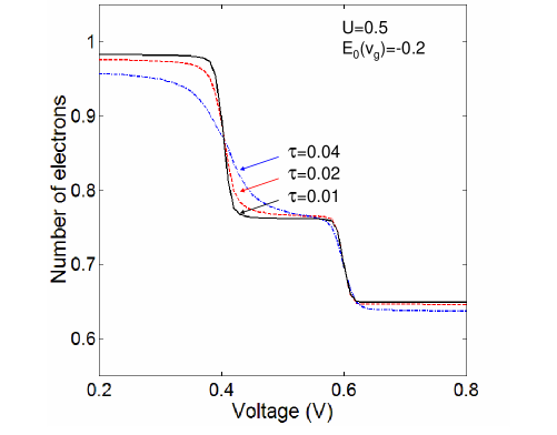
Figure 1: Average occupation numbers in the quantum dot as function of the voltage applied across the junction. The curves are plotted assuming $U=0.5eV,\ kT=0.00026eV,\ E_{0}(V_{g})=-0.2eV,\ \tau=0.01eV$ (solid line), $0.02eV$ (dash-dotted line) and $0.04eV$ (dashed line).

Figure 2: Current through a junction within the Coulomb blockade regime. The curves are plotted assuming $U=0.5eV,\ kT=0.00026eV,\ E_{0}(V_{g})=-0.2eV,\ \ \tau_{0}=0.04eV,\ \tau=0.01eV$ (solid line), $0.02eV$ (dash-dotted line) and $0.04eV$ (dashed line). The factor $\tau_{0}^{2}/\tau^{2}$ is introduced to bring all $I-V$ curves to the same scale. The ratio of heights of the two steps revealed in the curves equals $2:1.$

The current-voltage curves in the Fig. 2 show typical Coulomb blockade features, namely, two steps whose heights are related as $2:1.$ So, we see that the results concerning the electron transport through a quantum dot obtained employing the transition rates equations may be quantitatively reproduced within the NEGF formalism when the retarded and lesser Green’s functions are approximated by Eqs. 5, 13, and the explicit expression 21 for the occupation numbers is used. Therefore, the disagreement discussed in the begining of the present work may be successfully erased, and the consistency between the NEGF formalism and the transitions rates equations in the description of the Coulomb blockade regime could be restored beyond the Hartree-Fock approximation.

It is worthwhile to remark that particular values of the average occupation numbers on the dot are very responsive to the gate voltage value $V_{g}$ (the latter determines how the dot energy level is situated with respect to the Fermi levels of the leads in the absence of the voltage applied across them) and to the Coulomb interaction energy $U.$ Therefore, different values chosen for $V_{g}$ and $U$ lead to different average occupation numbers. However, under various assumptions for the $V_{g}$ and $U$ values, one quantity does not vary provided the symmetric coupling of the dot to the leads. This quantity is the relative height of the subsequent steps in the average occupation numbers of the electrons in the dot which are revealed as the voltage across the leads increases. As shown in the Fig. 1 this ratio is $2:1,$ exactly the same as for the subsequent current steps in the $I-V$ curves in the Fig. 2. And it is this ratio which ensures the correct shape of $I-V$ curves. For instance, comparing figure 1 with the corresponding result reported on the work 22 , one may see that the values of the occupation numbers given in Ref. 22 considerably differ from those obtained in the present work. Nevertheless, the ratio of the subsequent steps heights in the occupation numbers versus voltage curves is $2:1$, and this provides for the same ratio of heights of the subsequent current steps.

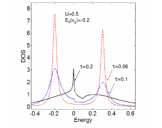
Figure 3: The equilibrium $(V=0)$ electron density of states in the quantum dot. The curves are plotted for $\tau=0.2eV$ (solid line) $0.1eV$ (dashed line) and $0.06eV$ (dash-dotted line). The remaining parameters are the same as those in the figure 1.

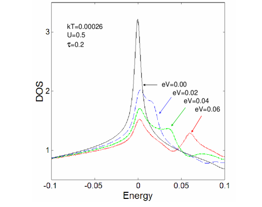
Figure 4: Splitting of the Kondo peak in the electron density of states with increasing bias. The curves are plotted for $eV=0$ (solid line); $0.02eV$ (dashed line), $0.04eV$ (dash-dotted line) and $0.06eV$ (dotted line). The coupling strength $\tau=0.2eV.$ The remaining parameters are taken as in the figures 1,2.

Also, the Eqs. 5, 13, 19 could be applied to analyze the Kondo effect which is manifested at stronger coupling strengths of the dot to the charge reservoirs. The electron density of states (DOS) in the dot is given as

$$D(E)=-2\sum_{\sigma}\mbox{Im}\left[G_{\sigma}^{rr}(E)\right].$$ (25)

Using $G_{\sigma}^{rr}(E)$ in the form 5 we may compute the electron DOS. The results are presented in the Fig. 3 where the equilibrium DOS is shown for three values of the coupling strength $\tau.$ For a sufficiently strong coupling of the dot to the source and drain reservoirs $(\tau=0.2eV)$ the sharp Kondo peak appears at $E=0,$ and the peaks at $E=E_{0}$ and $E=E_{0}+U$ are damped. At weaker coupling strength $(\tau=0.1eV,\ 0.07eV)$ the Kondo peak is reduced to a tiny feature but the maxima at $E=E_{0}$ and $E=E_{0}+U$ which determine the conductance within the Coulomb blockade regime emerge. The weaker is the coupling the higher become these peaks.

The heights of the peaks differ. Technically, this distinction originates from the fact that the value of $\big{<}n_{-\sigma}\big{>}$ in the expression for the retarded Green’s function (5) differs from $0.5.$ As shown in the book 19 , assuming $\big{<}n_{-\sigma}\big{>}=\big{<}n_{\sigma}\big{>}=0.5$ one would get the Coulomb blockade peaks of equal height but such assumption leads to the wrong result for the current. Namely, one would obtain two steps of equal height on the current voltage curves. The physical reason of this difference in the peak heights is the same as for the difference in heights of the steps on the current-voltage characteristics within the Coulomb blockade regime. The latter was discussed in the Introduction. When the voltage is applied across the junction the Kondo peak splits in two maxima whose heights are significantly smaller than the height of the original equilibrium Kondo peak and the greater is the voltage the lower these maxima become. This is shown in the Fig. 4. So, the present formalism sufficiently reproduces the results of earlier works concerning the Kondo effect (see e.g. Refs. 24 ; 25 ).

Finally, in the present work we theoretically analyzed the electron transport through a single quantum dot coupled to the source and drain charge reservoirs. The analysis was based on the NEGF formalism. The expression (5) for the retarded Green’s function was obtained using the equations of motion method, and agrees with the results of the previous works 21 ; 24 ; 25 . The lesser Green’s function was found from the Keldysh equation using the factor $\Sigma_{\sigma}^{<}$ in the form (12). This means that $\Sigma_{\sigma}^{<}$ is supposed to be unchanged due to the Coulomb interactions on the quantum dot, as it is proved to be within the Hartree-Fock approximation. We believe the proposed approximation to be appropriate at moderate and/or weak coupling of the dot to the leads when the coupling strengths are smaller than the characteristic Coulomb energy on the dot. We derived an explicit expression for the occupation numbers of electrons in the dot (Eq. 21) which enables us to compute them avoiding the long iterative procedure. The employed formalism gives correct results in the Coulomb blockade regime corroborating the results following from the transition rates (master) equations. Our approach is able to quantitatively reproduce the relative heights $(2:1)$ of the steps in the current voltage curves and to qualitatively describe the Kondo peak using the same expressions for the relevant Green’s functions. To the best of our knowledge this was never achieved so far.

Also, we remark that the present work addresses a general problem arising within the NEGF based computations. To quantitatively describe fine features of Kondo effect and related phenomena one needs to include hybridization up to very high orders in calculations of the relevant Green’s functions. Carrying out these cumbersome calculations where numerous approximations are inserted, it is easy to make a mistake and difficult to discover one, especially in the absence of obvious small parameters. Probably, such a mistake would not affect the very existence of the Kondo peak but it could distort its fine features. In the present work we propose a method which could help to verify the resulting expressions for the Green’s functions. We start from the clear point, namely, that the Green’s functions suitable to describe the Kondo effect are suitable to describe the Coulomb blockade transport, as well. Therefore, one may verify obtained results by going to the Coulomb blockade limit. If it occurs that particular Green’s functions fail to provide the correct form of the I-V curves within this limit then one must conclude that there is some error in the adopted approximations for the Green’s functions.

It is shown that calculational scheme employed in the present work which uses a very simple approximation for $G_{\sigma}^{<}$ brings quantitatively correct results for the electron transport through a quantum dot within the Coulomb blockade regime whereas advanced self-consistent calculations carried out in the recent paper 20 do not. This gives grounds to conjecture that it is not necessary (and, perhaps, it is not always correct) to use the same number of iterations in seeking approximations for retarded/advanced and the lesser Green’s functions within EOM method. Also, we remark that validity of the Green’s functions used in studies of the Kondo effect may be verified by applying them to calculate electron transport within the Coulomb blockade regime. The results could be generalized to include more realistic case of a dot including many electron levels, assuming that level separations are much greater than the Coulomb energy $U,$ so one may neglect Coulomb interactions of electrons belonging to different levels.

IV Acknowledgments:

Author thanks S. Datta for helpful discussions, and G. M. Zimbovsky for help with the manuscript. This work was supported by DoD grant W911NF-06-1-0519 and NSF-DMR-PREM 0353730.

V appendix

Here, we explain how the expression (5) for the Green’s function for the dot is derived. We introduce the following notation for a general retarded Green’s function Fourier component:

$$\big{<}\big{<}A,B\big{>}\big{>}\equiv-i\int_{0}^{\infty}\big{<}\{A(t);B\}\big{>}e^{i(E+i\eta)t}dt$$ (26)

where $A,B$ are operators, curly brackets denote the anticommutator and $\big{<}\cdots\big{>}$ stands for the average. For the Hamiltonian (1) the equation of motion for the retarded Green’s function for the dot $G_{\sigma}^{rr}(E)\equiv\big{<}\big{<}c_{\sigma};c_{\sigma}^{+}\big{>}\big{>}$ reads:

$$(E-E_{0}+i\eta)\big{<}\big{<}c_{\sigma};c_{\sigma}^{+}\big{>}\big{>}=1 +\sum_{r,\beta}\tau_{r\beta,\sigma}\big{<}\big{<}c_{r\beta\sigma};c_{\sigma}^{+}\big{>}\big{>}$$

$$+U\big{<}\big{<}n_{-\sigma}c_{\sigma};c_{\sigma}^{+}\big{>}\big{>}.$$ (27)

Here, $n_{-\sigma}\equiv c_{-\sigma}^{+}c_{-\sigma},$ and the Green’s function $\big{<}\big{<}c_{r\beta\sigma};c_{\sigma}^{+}\big{>}\big{>}$ obeys the equation:

$$(E-\epsilon_{r\beta\sigma}+i\eta)\big{<}\big{<}c_{r\beta\sigma};c_{\sigma}^{+}\big{>}\big{>}=\tau_{r\beta\sigma}^{*}\big{<}\big{<}c_{\sigma};c_{\sigma}^{+}\big{>}\big{>}.$$ (28)

Substituting the expression for $\big{<}\big{<}c_{r\beta\sigma};c_{\sigma}^{+}\big{>}\big{>}$ determined by 28 into 27 we get:

$$(E-E_{0}-\Sigma_{0\sigma})\big{<}\big{<}c_{\sigma};c_{\sigma}^{+}\big{>}\big{>}=1+U\big{<}\big{<}n_{-\sigma}c_{\sigma};c_{\sigma}^{+}\big{>}\big{>}$$ (29)

where the self-energy part $\Sigma_{0\sigma}$ is given by Eq. 6. The equation of motion for the four-operator function $\big{<}\big{<}n_{-\sigma}c_{\sigma};c_{\sigma}^{+}\big{>}\big{>}$ includes higher order Green’s functions. Omitting them we write out:

$$(E-E_{0}-U+i\eta)\big{<}\big{<}n_{-\sigma}c_{\sigma};c_{\sigma}^{+}\big{>}\big{>}$$

$$= \big{<}n_{-\sigma}\big{>}+\sum_{r,\beta}\Big{(}\tau_{r\beta\sigma}\big{<}\big{<}c_{r\beta\sigma}n_{-\sigma};c_{\sigma}^{+}\big{>}\big{>}+\tau_{r\beta;-\sigma}\big{<}\big{<}c_{-\sigma}^{+}c_{r\beta;-\sigma}c_{\sigma};c_{\sigma}^{+}\big{>}\big{>}-\tau_{r\beta;-\sigma}^{*}\big{<}\big{<}c_{r\beta;-\sigma}c_{-\sigma}c_{\sigma};c_{\sigma}^{+}\big{>}\big{>}\Big{)}.$$ (30)

To proceed we must write equations for the Green’s functions inserted in the right side of the Eq. 30. We get:

$$(E-\epsilon_{r\beta\sigma}+i\eta)\big{<}\big{<}c_{r\beta\sigma}n_{-\sigma};c_{\sigma}^{+}\big{>}\big{>}$$

$$= \tau_{r\beta\sigma}^{*}\big{<}\big{<}n_{-\sigma}c_{\sigma};c_{\sigma}^{+}\big{>}\big{>}+\sum_{r^{\prime}\beta}\big{(}\tau_{r^{\prime}\beta;-\sigma}\big{<}\big{<}c_{r\beta\sigma}c_{-\sigma}^{+}c_{r^{\prime}\beta;-\sigma};c_{\sigma}^{+}\big{>}\big{>}-\tau_{r^{\prime}\beta;-\sigma}^{*}\big{<}\big{<}c_{r^{\prime}\beta-\sigma}c_{-\sigma}c_{r\beta;\sigma};c_{\sigma}^{+}\big{>}\big{>}\big{)},$$ (31)

$$(E-\epsilon_{r\beta;-\sigma}+i\eta)\big{<}\big{<}c_{-\sigma}^{+}c_{r\beta;-\sigma}c_{\sigma};c_{\sigma}^{+}\big{>}\big{>}$$

$$= \tau_{r\beta;-\sigma}^{*}\big{<}\big{<}n_{-\sigma}c_{\sigma};c_{\sigma}^{+}\big{>}\big{>}-\sum_{r^{\prime}\beta}\big{(}\tau_{r^{\prime}\beta-\sigma}\big{<}\big{<}c_{r^{\prime}\beta;-\sigma}^{+}c_{r\beta;-\sigma}c_{\sigma};c_{\sigma}^{+}\big{>}\big{>}+\tau_{r^{\prime}\beta\sigma}\big{<}\big{<}c_{-\sigma}^{+}c_{r\beta;-\sigma}c_{r^{\prime}\beta\sigma};c_{\sigma}^{+}\big{>}\big{>}\big{)},$$ (32)

$$(E-2E_{0}-U+\epsilon_{r\beta;-\sigma}+i\eta)\big{<}\big{<}c_{r\beta;-\sigma}^{+}c_{-\sigma}c_{\sigma};c_{\sigma}^{+}\big{>}\big{>}$$

$$= -\tau_{r\beta;-\sigma}\big{<}\big{<}n_{-\sigma}c_{\sigma};c_{\sigma}^{+}\big{>}\big{>}+\sum_{r^{\prime}\beta}\big{(}\tau_{r^{\prime}\beta\sigma}\big{<}\big{<}c_{r^{\prime}\beta;-\sigma}^{+}c_{-\sigma}c_{r\beta\sigma};c_{\sigma}^{+}\big{>}\big{>}-\tau_{r^{\prime}\beta;-\sigma}\big{<}\big{<}c_{r\beta;-\sigma}^{+}c_{\sigma}c_{r^{\prime}\beta;-\sigma};c_{\sigma}^{+}\big{>}\big{>}\big{)}.$$ (33)

Writing out these equations 31-33 we neglected averages like $\big{<}c_{\sigma}^{+}c_{r\beta\sigma}\big{>}$ including a creation/annihilation operator for the dot combined with the annihilation/creation operator for the source/drain reservoir. Such averages are omitted in further calculations, as well. Now, we decouple four-operator Green’s functions included in the sums over $``r^{\prime}"$ in the equations following the scheme 26 :

$$\big{<}\big{<}A^{+}BC;D^{+}\big{>}\big{>}\approx\big{<}A^{+}B\big{>}\big{<}\big{<}C;D^{+}\big{>}\big{>}-\big{<}A^{+}C\big{>}\big{<}\big{<}B;D^{+}\big{>}\big{>}.$$ (34)

Also, we use the approximation:

$$\big{<}c_{r\beta\sigma}^{+}c_{r^{\prime}\beta\sigma}\big{>}=\big{<}c_{r^{\prime}\beta\sigma}c_{r\beta\sigma}^{+}\big{>}=\delta_{rr^{\prime}}f_{r\sigma}^{\beta}$$ (35)

where $f_{r\sigma}^{\beta}$ is the Fermi distribution function corresponding to the energy $\epsilon_{r\beta\sigma}.$ As a result, the Green’s functions included in the right-hand side of the Eq. 30 get expressed in terms of the Green’s functions $\big{<}\big{<}n_{-\sigma}c_{\sigma};c_{\sigma}^{+}\big{>}\big{>}$ and $\big{<}\big{<}c_{\sigma};c_{\sigma}^{+}\big{>}\big{>}.$ Substituting these expressions into Eq. 30 we obtain:

$$\big{<}\big{<}n_{-\sigma}c_{\sigma};c_{\sigma}^{+}\big{>}\big{>}=\frac{\big{<}n_{-\sigma}\big{>}+\Sigma_{1\sigma}\big{<}\big{<}c_{\sigma};c_{\sigma}^{+}\big{>}\big{>}}{E-E_{0}-U-\Sigma_{02}^{\sigma}}.$$ (36)

Here, self-energy parts $\Sigma_{1\sigma},\Sigma_{2\sigma},\Sigma_{02}^{\sigma}$ are given by:

$$\Sigma_{1\sigma}= \sum_{r\beta}|\tau_{r\beta,-\sigma}|^{2}f_{r,-\sigma}^{\beta}\left\{\frac{1}{E-2E_{0}-U+\epsilon_{r\beta,-\sigma}+i\eta}\right.$$

$$+\left.\frac{1}{E-\epsilon_{r\beta,-\sigma}+i\eta}\right\},$$ (37)

$$\Sigma_{2\sigma}= \sum_{r\beta}|\tau_{r\beta,-\sigma}|^{2}\left\{\frac{1}{E-2E_{0}-U+\epsilon_{r\beta,-\sigma}+i\eta}\right.$$

$$+\left.\frac{1}{E-\epsilon_{r\beta,-\sigma}+i\eta}\right\},$$ (38)

$$\Sigma_{02}^{\sigma}=\Sigma_{0\sigma}+\Sigma_{2\sigma}.$$ (39)

To arrive at the resulting expression for the dot Green’s function $G_{\sigma}^{rr}\equiv\big{<}\big{<}c_{\sigma};c_{\sigma}^{+}\big{>}\big{>}$ we substitute Eq. 36 into Eq. 29. We have:

$$G_{\sigma}^{rr}(E)=\frac{E-E_{0}-\Sigma_{02}^{\sigma}-U(1-\big{<}n_{-\sigma}\big{>})}{(E-E_{0}-\Sigma_{0\sigma})(E-E_{0}-U-\Sigma_{02}^{\sigma})+U\Sigma_{1\sigma}}.$$ (40)

References

- (1) M. A. Kastner, Rev. Mod. Phys. 64, 849 (1992).
- (2) L. I. Glazman and M. E. Raikh, JETP Lett. 47, 452 (1988).
- (3) T. K. Ng and P. A. Lee, Phys. Rev. Lett. 61, 1768 (1988).
- (4) J. Park, A. N. Pasupathy, J. I. Goldsmith, C. Chang, Y. Yaish, J. R. Petta, M. Rinkovski, J. P. Sethna, H. D. Abruna, P. I. McEuen, and D. C. Ralph, Nature 417, 722 (2002).
- (5) W. Liang, M. P. Shores, M. Bockrath, J. R. Long, and H. Park, Nature 417, 725 (2002).
- (6) N. B. Zhitenev, H. Meng, and Z. Bao, Phys. Rev. Lett. 88, 226801 (2002).
- (7) J. Reichert, H. B. Weber, M. Mayor, and H. v. Lohneysen, Appl. Phys. lett. 82, 4137 (2003).
- (8) L. H. Yu and D.l Natelson, Nano Lett. 4, 79 (2004).
- (9) L. H. Yu, Z. K. Keane, J. W. Ciszek, L. Cheng, M. P. Stewart, J. M. Tour, and D. Natelson, Phys. Rev. Lett. 93, 266802 (2004).
- (10) D. Porath and O. Millo, J. Appl. Phys. 81, 2241 (1997).
- (11) M. Dorogi, J. Gomez, R. Osifchin, R. P. Andres, and R. Reifenberger, Phys. Rev. B 52, 9071 (1995).
- (12) Y. O. Feng, R. Q. Zhang, and S. T. Lee, J. Appl. Phys. 95, 5729 (2004).
- (13) B. I. Leroy, S. G. Lemay, J. Kong, and C. Dekker, Nature 395, 371 (2004).
- (14) K. Grove-Rasmussen, H. I. Jorgensen, and P. E. Lindelof, arXiv:07111922 [cond-mat].
- (15) D. V. Averin and K. K. Likharev, J. Low. Temp. Phys. 62, 345 (1986).
- (16) D. V. Averin, A. N. Korotkov, and K. K. Likharev, Phys. Rev. B 44, 6199 (1991).
- (17) S. A. Gurvitz, D. Mozyrsku, and G. P. Berman, Phys. Rev. B 72, 205341 (2005).
- (18) B. Muralidharan, A. W. Ghosh, and S. Datta, Phys. Rev. B 73, 155410 (2006).
- (19) S. Datta, Quantum Transport: Atom to Transistor (Cambridge University Press, 2005).
- (20) See M. Galperin, A. Nitzan, and M. Ratner, Phys. Rev. B 76, 035301 (2007) and references therein.
- (21) Y. Meir, N. S. Wingreen, and P. A. Lee, Phys. Rev. Lett. 66, 3048 (1991).
- (22) R. Swirkowics, J. Barnas and M. Wilczynski, J. Phys: Condens. Matter 14, 2011 (2002).
- (23) P. Pals and Mackinnon, J. Phys: Condens. Matter 8, 5401 (1996).
- (24) Y. Meir, N. S. Wingreen, and P. A. Lee, Phys. Rev. Lett. 70, 2601 (1993).
- (25) R. Swirkowics, J. Barnas, and M. Wilczynski, Phys. Rev. B 68, 195318 (2003).
- (26) V Kascheyev, A. Aharony, and O. Entin-Wolhlman, Phys. Rev. B 73, 125338 (2006).
- (27) A similar way of the occupation numbers calculations was recently proposed by Galperin et al 20 .
- (28) A.-P. Jauho, N. S. Wingreen, and Y. Meir, Phys. Rev. B 50, 5528 (1994).
- (29) H. Hang and A.-P. Jauho, Quantum Kinetics in Transport and Optics in Semiconductors, (Springer, berlin, 1996).