Constraints on Dark Energy from Galaxy Cluster Gas Mass Fraction versus Redshift data

Abstract

We use the Allen et al. (2008) galaxy cluster gas mass fraction versus redshift data to constrain parameters of three different dark energy models: a cosmological constant dominated one ($\Lambda$CDM); the XCDM parameterization of dark energy; and a slowly-rolling scalar field model with inverse-power-law potential energy density. (Instead of using the Monte Carlo Markov Chain method, when integrating over nuisance parameters we use an alternative method of introducing an auxiliary random variable.) The resulting constraints are consistent with, and typically more constraining than, those derived from other cosmological data. A time-independent cosmological constant is a good fit to the galaxy cluster data, but slowly evolving dark energy cannot yet be ruled out.

1 Introduction

Observations over the last decade have established that the cosmological expansion is accelerating. In the context of general relativity this requires that the cosmological energy budget be dominated by dark energy (for reviews see, e.g., Copeland et al., 2006; Padmanabhan, 2006; Ishak, 2007; Uzan, 2007; Linder, 2007; Ratra & Vogeley, 2008). This hypothetical construct — dark energy — is an enigma. It is not yet clearly established whether dark energy is Einstein’s cosmological constant $\Lambda$ (e.g., Peebles, 1984), or whether it evolves slowly in time and varies weakly in space (e.g., Peebles & Ratra, 1988; Ratra & Peebles, 1988). While Type Ia supernova (SNIa) apparent magnitude measurements as a function of redshift indicate accelerated cosmological expansion (Riess et al., 1998; Perlmutter et al., 1999), SNIa data are as yet unable to unambiguously constrain dark energy (see, e.g., Alam et al., 2007; Nesseris & Perivolaropoulos, 2007; Shafieloo, 2007; Zhang et al., 2007; Wu et al., 2008; Ishida et al., 2008). Future SNIa data will improve the constraints (e.g., Podariu et al., 2001a) and could resolve some of the current differences in results from different SNIa data sets.

The results of the SNIa test are confirmed by a test based on cosmic microwave background (CMB) anisotropy data that must assume the cold dark matter (CDM) model for structure formation (see Peebles & Ratra 2003 and references therein for a discussion of apparent problems with the CDM model). CMB anisotropy data is consistent with the Universe having negligible spatial curvature (see, e.g., Podariu et al., 2001b; Durrer et al., 2003; Mukherjee et al., 2003; Page et al., 2003; Spergel et al., 2007; Doran et al., 2007a), under the assumption that dark energy does not evolve in time (e.g., Wright, 2006; Tegmark et al., 2006; Zhao et al., 2007; Ichikawa & Takahashi, 2007; Wang & Mukherjee, 2007). In combination with low measured non-relativistic matter density (Chen & Ratra 2003b and references therein), negligible spatial hypersurface curvature indicates the presence of dark energy.

There are many different models of dark energy. In this paper we consider three: standard $\Lambda$CDM, the XCDM parameterization, and a slowly rolling scalar field dominated one ($\phi$CDM). In the $\Lambda$CDM model the late-time Universe is dominated by a cosmological constant $\Lambda$ with time-independent energy density $\rho_{\Lambda}$ (Peebles, 1984). In $\phi$CDM the dark energy is a slowly rolling scalar field $\phi$; in the model we consider the scalar field potential energy density $V(\phi)\propto\phi^{-\alpha}$, where $\alpha$ is a nonnegative parameter (Peebles & Ratra, 1988). We also consider the XCDM parameterization of the dark energy equation of state; here dark energy is modeled as a fluid with an equation of state which relates the fluid pressure $p=\omega_{\rm x}\rho$ to its energy density $\rho$ where $\omega_{\rm x}$ is a time-independent negative parameter. This approximation is inaccurate in the scalar field dominated epoch (Ratra, 1991). In all three models, other contributors to the Universe’s current energy budget include CDM and baryonic matter. In the $\phi$CDM and XCDM cases spatial hypersurfaces are taken to be flat, while spatial curvature is treated as a cosmological parameter in the $\Lambda$CDM model we consider.

It is important to confirm and strengthen the SNIa and CMB test results by using additional techniques. This will allow for consistency checks as well as possibly identifying systematic effects in a particular data set. Other promising current tests include the angular size of radio sources and quasars as a function of redshift (e.g., Chen & Ratra, 2003a; Podariu et al., 2003; Daly & Djorgovski, 2005; Daly et al., 2007), strong gravitational lensing (e.g., Chae et al., 2004; Alcaniz et al., 2005; Fedeli & Bartelmann, 2007; Lee & Ng, 2007; Oguri et al., 2008), measurements of the Hubble parameter as a function of redshift (e.g., Samushia & Ratra, 2006; Sen & Scherrer, 2008; Lazkoz & Majerotto, 2007; Wei & Zhang, 2007; Samushia et al., 2007), and large-scale structure baryon acoustic oscillation measurements (e.g., Doran et al., 2007b; Parkinson et al., 2007; Percival et al., 2007; Lima et al., 2007). For reviews of the observational situation see Kurek & Szydłowsky (2008), Wang (2007b), and Lazkoz et al. (2007). Current data favor dark energy that does not evolve, but do not yet strongly rule out evolving dark energy (see, e.g., Rapetti et al., 2005; Wilson et al., 2006; Davis et al., 2007).

In this paper we use new galaxy cluster gas mass fraction versus redshift data (Allen et al., 2008, hereafter A08) to constrain parameters of the three dark energy models mentioned above. Earlier galaxy cluster gas mass fraction data (Allen et al., 2004) have been used to constrain these and other models (e.g., Chen & Ratra, 2004; Rapetti et al., 2005; Alcaniz et al., 2005; Cannata & Kamenshchik, 2006; Zhan, 2006; Wei & Zhang, 2007).

If rich galaxy clusters are large enough to have matter content that fairly samples that of the Universe then the baryonic to total mass ratio in clusters is equal to the cosmological baryonic mass fraction ratio of $\Omega_{\rm b}$ and $\Omega_{\rm m}$, the baryonic and nonrelativistic mass density parameters. The baryonic mass in clusters is dominated by the x-ray emitting gas which can be measured through x-ray observations. Combined with an estimate of $\Omega_{\rm b}$ from other observations, these measurements can be used to constrain $\Omega_{\rm m}$. The gas mass fraction in large relaxed clusters is expected to be independent of redshift and, since the observed x-ray temperature depends on the assumed distance to the cluster, this can be used to constrain cosmological parameters (Sasaki, 1996; Pen, 1997; for recent discussions of the test see, e.g., Ettori et al., 2006; Nagai et al., 2007; Crain et al., 2007).

In addition to depending on cosmological parameters, in a given model the predicted gas mass fraction depends on a number of “nuisance” parameters that have to be marginalized over to derive the probability distribution function for the cosmological parameters of interest. We note that the likelihood function depends on certain functions of the “nuisance” parameters and so introduce auxiliary random variables to describe these functions. This technique helps us to significantly reduce the computational time.

In next section we outline our computations. In Sec. 3 we present and discuss our results and conclude.

2 Computation

In our computations we follow A08. For a given cosmological model we compute predicted values of the gas mass fraction

$$f_{\rm gas}^{\rm th}(z,h,\Omega_{\rm m},p,\Omega_{\rm b},Q)=\frac{KA\gamma b_{0}(1+\alpha_{b}z)}{1+s_{0}(1+\alpha_{s}z)}\left(\frac{\Omega_{\rm b}}{\Omega_{\rm m}}\right)\left[\frac{d_{\rm A}^{\Lambda}(z)}{d_{\rm A}(z)}\right]^{1.5},$$ (1)

as a function of cluster redshift $z$, 4 cosmological parameters ($h,\Omega_{\rm m},\Omega_{\rm b}$, and a parameter $p$, described below, that represents the dark energy model), and 7 parameters ($s_{0}$, $b_{0}$, $\alpha_{s}$, $\alpha_{b}$, $K$, $A$, $\gamma$) represented by $Q$ and related to modeling the cluster gas mass fraction. Here $h$ is the Hubble parameter in units of 100 $\rm kms^{-1}Mpc^{-1}$, $d_{\rm A}^{\Lambda}(z)$ is the angular diameter distance computed in the reference spatially-flat $\Lambda\rm{CDM}$ model (with $\Omega_{\rm m}=0.3$, $\Omega_{\Lambda}=0.7$, and $h=0.7$, where $\Omega_{\Lambda}$ is the cosmological constant density parameter), and $d_{\rm A}(z)$ is the angular diameter distance computed in the cosmological model of interest and depends on the model and $h$. Since the angular diameter distance $d_{\rm A}(z)$, and so $f_{\rm gas}^{\rm th}$, depends on the assumed dark energy model, we can compare predicted values of the gas mass fraction with measurements for clusters at redshift $z_{i}$ by constructing a $\chi^{2}=\sum_{i}(f_{\rm gas}^{\rm th}(z_{i})-f_{\rm gas}^{\rm obs}(z_{i}))^{2}/\sigma_{i}^{2}$ function ($\sigma_{i}$ are the one standard deviation measurement errors and the summation is over the 42 A08 clusters), and so constrain parameters of given dark energy models.

We construct a likelihood function $L=e^{-\chi^{2}/2}$, which depends on cosmological parameters like $\Omega_{\rm m}$ and those describing the dark energy model, as well as on the nuisance parameters. We marginalize over the nuisance parameters by multiplying the likelihood by the probability distribution function for the nuisance parameters and then integrating (e.g., Ganga et al., 1997). The resulting probability distribution function depends only on two variables: $\Omega_{m}$ and a parameter $p$ describing the dark energy model. In the $\Lambda$CDM case $p$ is $\Omega_{\Lambda}$, in XCDM it is $\omega_{\rm x}$, and in $\phi$CDM it is $\alpha$. Since we consider only spatially-flat cosmologies for XCDM and $\phi$CDM models, two parameters $p$ and $\Omega_{m}$ completely describe the background evolution.

Since our initial likelihood function depends on 10 parameters in total (after setting $A=1$), to get to the two-dimensional probability distribution function we have to marginalize over 8 nuisance parameters ($h$, $\Omega_{\rm b}$, and the 6 parameters used to model the cluster gas mass fraction). To reduce computational time we use the following statistics results (see, e.g., Riley et al., 2002, chap. 26). If two random variables $a$ and $b$ are independent and have probability distribution functions $P_{a}(x)$ and $P_{b}(x)$, then variables $c=ab$, $d=a/b$, and $f=F(a)$ are also random with probability distribution functions

$$P_{c}(x)=\int{\int{P_{a}(x^{\prime})P_{b}(x^{\prime\prime})\delta(x^{\prime}x^{\prime\prime}-x)dx^{\prime}dx^{\prime\prime}}}=\int{\frac{1}{|x^{\prime}|}P_{a}(x^{\prime})P_{b}(x/x^{\prime})dx^{\prime}},$$ (2)

$$P_{d}(x)=\int{\int{P_{a}(x^{\prime})P_{b}(x^{\prime\prime})\delta(x^{\prime}/x^{\prime\prime}-x)dx^{\prime}dx^{\prime\prime}}}=\int{|x^{\prime}|P_{a}(xx^{\prime})P_{b}(x^{\prime})dx^{\prime}},$$ (3)

$$P_{f}(x)=\left|\frac{dF^{-1}(x)}{dx}\right|P_{a}(F^{-1}(x)),$$ (4)

where $\delta(x)$ is a Dirac delta function. For example, since $d_{\rm A}$ in Eq. (1) is inversely proportional to $h$, we define an auxiliary variable $\Upsilon=K\gamma b_{0}(\Omega_{\rm b}h^{2})/\sqrt{h}$ and numerically compute a probability distribution function for it. This allows us to replace a five-dimensional integration (over $K$, $\gamma$, $b_{0}$, $\Omega_{\rm b}h^{2}$, and $h$) by a one-dimensional integral over a new variable $\Upsilon$ and so reduce computational time significantly.

Prior probability distribution functions for nuisance parameter are given in Table 1. The distribution functions for the 6 cluster gas mass fraction parameters are given A08, Table 4. Best fit values and confidence level constraints on dark energy parameters are sensitive to the assumed priors for the baryonic mass density and the Hubble parameter. Since different experiments give somewhat different estimates of these two, in our paper we use two prior sets to illustrate the differences. One set is from WMAP 3 year cumulative data (Spergel et al., 2007), $h=0.73\pm 0.03$ and $\Omega_{\rm b}h^{2}=0.0223\pm 0.0008$, one standard deviation errors. The alternate set of priors we use is $h=0.68\pm 0.04$ (Gott et al., 2001; Chen et al., 2003) and $\Omega_{\rm b}h^{2}=0.0205\pm 0.0018$ (Fields & Sarkar, 2006), one standard deviation errors.

We define best fit values as pairs of values of cosmological parameters for which the likelihood function reaches its maximum. 1, 2, and 3 $\sigma$ confidence level contours are defined as sets of points in the parameter space with likelihood equal to $e^{-2.30/2}$, $e^{-6.17/2}$, and $e^{-11.8/2}$ of the maximum value of the likelihood respectively.

3 Results and Discussion

As a test we computed confidence level contours using our technique and the same prior set A08 used for $\Lambda$CDM and XCDM, Figs. 6 and 8 of A08. Our contours are in good agreement with those of A08.

Figures 1 to 3 show cluster gas mass fraction confidence level contours and best fit values for the three dark energy models and the two sets of priors for $\Omega_{\rm b}h^{2}$ and $h$ given in Table  1. Compared to the constraints derived from the earlier Allen et al. (2004) cluster gas mass fraction data (Chen & Ratra, 2004), the difference between the contours corresponding to the two prior sets (for $\Omega_{\rm b}h^{2}$ and $h$) is much reduced. The new constraints are almost as restrictive as the ones derived from SNIa data and more constraining than those derived from angular size versus redshift data or Hubble parameter versus redshift data.

Figure 1 shows constraints on $\Lambda$CDM. $\Omega_{\rm m}$ is better constrained than $\Omega_{\Lambda}$ and the results are in good qualitative accord with previous analyses. The best fit values are slightly away from a spatially-flat model.

Figure 2 shows constraints on the XCDM parameterization. Again, the energy density of nonrelativistic matter is fairly well constrained while the equation of state parameter is less constrained. The best fit values are again not exactly on the $\omega_{\rm x}=-1$ line, which corresponds to the spatially-flat $\Lambda$CDM case.

Figure 3 shows constraints on the $\phi$CDM model. $\Omega_{\rm m}$ is better constrained than $\alpha$. For both sets of priors there is an upper limit on $\alpha$. The best fit values are on the $\alpha=0$ line which corresponds to the spatially-flat $\Lambda$CDM case, but there is a big part of evolving dark energy parameter space that still is not ruled out.

Table 1: Prior probability distribution functions for nuisance parameters

	Parameter	Allowance	Distribution
WMAP prior $\Omega_{\rm b}h^{2}$	$\Omega_{\rm b}h^{2}$	$0.0223\pm 0.0008$	Gaussian
WMAP prior $h$	$h$	$0.73\pm 0.03$	Gaussian
Alternate prior $\Omega_{\rm b}h^{2}$	$\Omega_{\rm b}h^{2}$	$0.0205\pm 0.0018$	Gaussian
Alternate prior $h$	$h$	$0.68\pm 0.04$	Gaussian

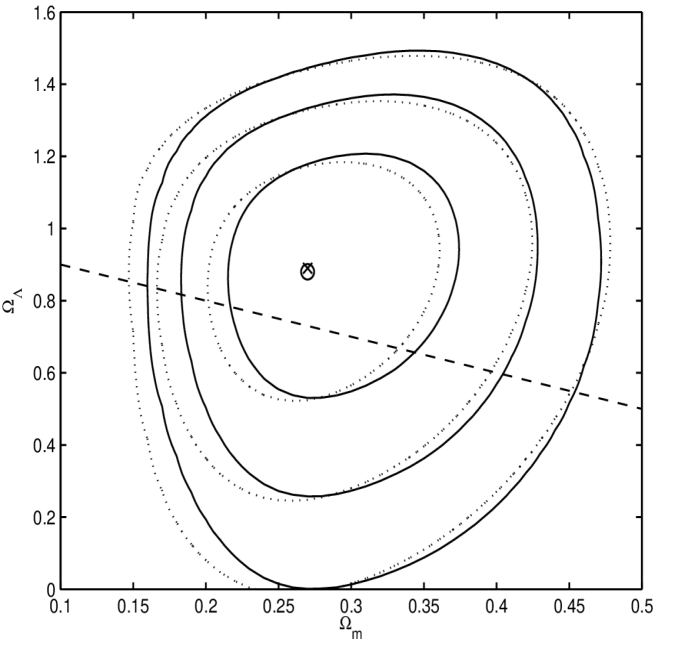
Figure 1: 1, 2, and 3$\sigma$ confidence level contours for the $\Lambda$CDM model. Solid lines ($\times$ for the best fit at $\Omega_{\rm m}=0.27$, $\Omega_{\Lambda}=0.89$) correspond to the WMAP prior and dotted lines ($\circ$ for the best fit at $\Omega_{\rm m}=0.27$, $\Omega_{\Lambda}=0.88$) correspond to the alternate prior. Dashed $\Omega_{\Lambda}=1-\Omega_{\rm m}$ line corresponds to the spatially-flat $\Lambda$CDM model.

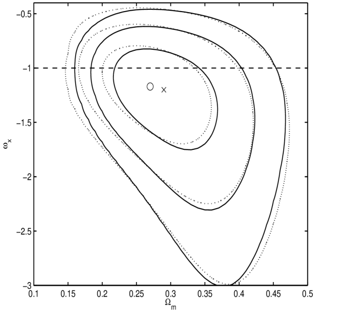
Figure 2: 1, 2, and 3$\sigma$ confidence level contours for the XCDM parameterization. Solid lines ($\times$ for the best fit at $\Omega_{\rm m}=0.29$, $\omega_{\rm x}=-1.2$) correspond to the WMAP prior and dotted lines ($\circ$ for the best fit at $\Omega_{\rm m}=0.27$, $\omega_{\rm x}=-1.17$) correspond to the alternate prior. Dashed $\omega_{\rm x}=-1$ line corresponds to the spatially-flat $\Lambda$CDM model.

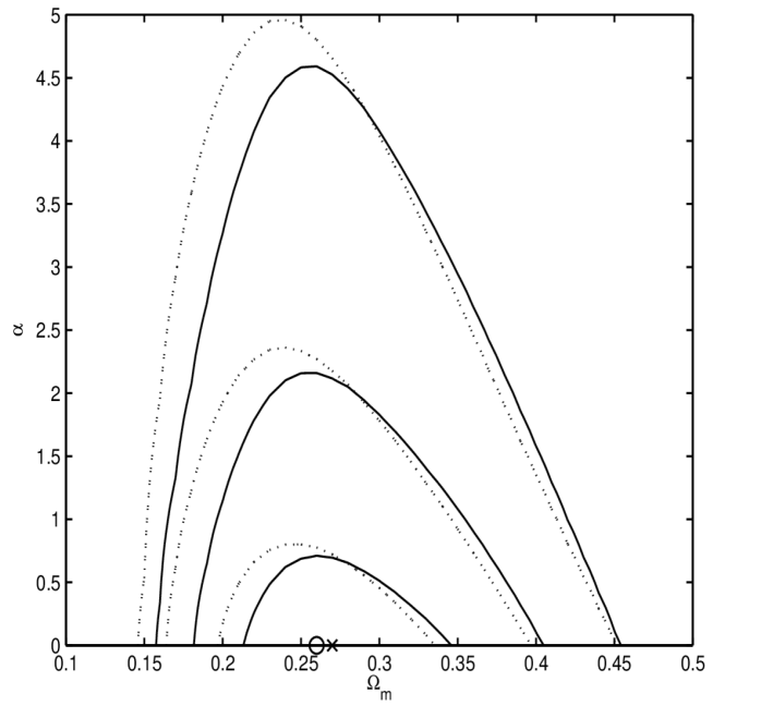
Figure 3: 1, 2, and 3$\sigma$ confidence level contours for the $\phi$CDM model. Solid lines ($\times$ for the best fit at $\Omega_{\rm m}=0.27$, $\alpha=0.0$) correspond to the WMAP prior and dotted lines ($\circ$ for the best fit at $\Omega_{\rm m}=0.26$, $\alpha=0.0$) correspond to the alternate prior. The $\alpha=0$ horizontal line corresponds to the spatially-flat $\Lambda$CDM model.

References

- Alam et al. (2007) Alam, U., Sahni, V., & Starobinsky. A. A. 2007, J. Cosmology Astropart. Phys, 0702, 011
- Alcaniz et al. (2005) Alcaniz, J. S., Dev. A., & Jain. D. 2005, ApJ, 627, 26
- Allen et al. (2008) Allen, S. W. et al. 2008, MNRAS, 383, 879 (A08)
- Allen et al. (2004) Allen, S. W. et al. 2004, MNRAS, 353, 457
- Amendola et al. (2007) Amendola, L., Charmousis, C., & Davis, S. C. 2007, J. Cosmology Astropart. Phys, 0710, 004
- Barenboim & Lykken (2006) Barenboim, G., & Lykken, J. D. 2006, J. High Energy Phys., 0607, 016
- Bonometto et al. (2006) Bonometto, S.A., Casarini, L., Colombo, L.P.L., & Mainini, R. 2006, arXiv:astro-ph/0612672
- Brax & Martin (2007) Brax, P., & Martin, J. 2007, Phys. Lett. B, 647, 320
- Cannata & Kamenshchik (2006) Cannata, F., & Kamenshchik, A. 2006, arXiv:gr-qc/0603129
- Chae et al. (2004) Chae, K.-H., Chen, G., Ratra, B., & Lee, D.-W. 2004, ApJ, 607, L71
- Chen et al. (2003) Chen, G., Gott, J. R., & Ratra, B. 2003, PASP, 115, 1269
- Chen & Ratra (2003a) Chen, G., & Ratra, B. 2003a, ApJ, 582, 586
- Chen & Ratra (2003b) Chen, G., & Ratra, B. 2003b PASP, 115, 1143
- Chen & Ratra (2004) Chen, G., & Ratra, B. 2004, ApJ, 612, L1
- Copeland et al. (2006) Copeland, E. J., Sami, M., & Tsujikawa, S. 2006, Int. J. Mod. Phys. D15, 753
- Crain et al. (2007) Crain, R. A., et al. 2007, MNRAS, 377, 41
- Daly & Djorgovski (2005) Daly, R. A., & Djorgovski, S. G. 2005, arXiv:astro-ph/0512576
- Daly et al. (2007) Daly.,R.,A., et al. 2007, arXiv:0710.5112 [astro-ph]
- Davis et al. (2007) Davis, T. M., et al. 2007, ApJ, 666, 716
- Demianski et al. (2007) Demianski, M., Piedipalumbo, E., Rubano, C., & Scudellaro, B. 2007, arXiv:0711.1043 [astro-ph]
- Doran et al. (2007b) Doran, M., Stern, S., & Thommes, E., 2007b, J. Cosmology Astropart. Phys, 0704, 015
- Doran et al. (2007a) Doran, M., Robbers, G., & Wetterich, C. 2007a, Phys. Rev. D, 75, 023003
- Durrer et al. (2003) Durrer, R., Novosyadlyj, B., & Apunevych, S. 2003, ApJ, 583, 33
- Dutta & Sorbo (2007) Dutta, K., & Sorbo, L. 2007, Phys. Rev. D, 75, 063514
- Ettori et al. (2006) Ettori, S., Dolag, K., Borgani, S., & Murante, G. 2006, MNRAS, 365, 1021
- Fay et al. (2007) Fay, S., Nesseris, S., & Perivolaropoulos, L. 2007, Phys. Rev. D, 76, 063504
- Fedeli & Bartelmann (2007) Fedeli, C., & Bartelmann, M. 2007, A&A, 461, 49
- Fields & Sarkar (2006) Fields, B. D., & Sarkar, S. 2006, J. Phys. G., 33, 220
- Ganga et al. (1997) Ganga, K., Ratra, B., Gunderson, J. O., & Sugiyama, N. 1997, ApJ, 484, 7
- Gott et al. (2001) Gott, J. R., Vogeley, M. S., Podariu, S., & Ratra, B. 2001, ApJ, 549, 1
- Grande et al. (2007) Grande, J., Opher, R., Pelinson, A., & Solà, J. 2007, J. Cosmology Astropart. Phys, 0712, 007
- Guo et al. (2007) Guo, Z.-K., Ohta, N., & Tsujikawa. S., 2007, Phys. Rev. D, 76, 023508
- Ichikawa & Takahashi (2007) Ichikawa, K. & Takahashi, T. 2007, J. Cosmology Astropart. Phys, 0702, 001
- Ishak (2007) Ishak. M., 2007, Found. Phys., 37, 1470
- Ishida et al. (2008) Ishida, É. E. O., Reis, R. R. R., Toribo, A. V. & Waga, I. 2008, Astropart. Phys., 28, 547
- Kurek & Szydłowsky (2008) Kurek, A., & Szydłowski, M., 2008, ApJ, 675, 1
- Lazkoz & Majerotto (2007) Lazkoz, R. & Majerotto, E. 2007, J. Cosmology Astropart. Phys, 0707, 015
- Lazkoz et al. (2007) Lazkoz, R., Nesseris, S., & Perivolaropulos, L. 2007, arXiv:0712.1232 [astro-ph]
- Lee & Ng (2007) Lee., S. & Ng, K.-W. 2007, Phys. Rev. D, 76, 043518
- Lima et al. (2007) Lima, J. A. S., Jesus, J. F., & Cunha, J. V. 2007, arXiv:0709.2195 [astro-ph]
- Linder (2007) Linder, E. V. 2007, arXiv:0704.2064 [astro-ph]
- Movahed et al. (2007) Movahed, M. S., Farhang, M., & Rahvar, S. 2007, arXiv:astro-ph/0701339
- Mukherjee et al. (2003) Mukherjee, P., et al. 2003, Int. J. Mod. Phys. A, 18, 4933
- Nagai et al. (2007) Nagai, D., Vikhlinin, A., & Kravtsov, A. V. 2007, ApJ, 655, 98
- Nesseris & Perivolaropoulos (2007) Nesseris, S., & Perivolaropoulos, L. 2007, J. Cosmology Astropart. Phys, 0702, 025
- Neupane & Scherer (2007) Neupane, I. P., & Scherer, C. 2007, arXiv:0712.2468 [astro-ph]
- Oguri et al. (2008) Oguri, M., et al. 2008, AJ, 135, 512
- Olivares et al. (2008) Olivares, G., Atrio-Barandela, F., & Pavón, D. 2008, Phys. Rev. D, 77, 063513
- Padmanabhan (2006) Padmanabhan, T. 2006, AIP Conf. Proc., 861, 174
- Page et al. (2003) Page, L., et al. 2003, ApJS, 148, 233
- Parkinson et al. (2007) Parkinson, D., et al. 2007, MNRAS, 377, 185
- Peebles (1984) Peebles, P. J. E. 1984, ApJ, 284, 439
- Peebles & Ratra (1988) Peebles, P. J. E., & Ratra, B. 1988, ApJ, 325, L17
- Peebles & Ratra (2003) Peebles, P. J. E., & Ratra, B. 2003, Rev. Mod. Phys., 75, 559
- Pen (1997) Pen, U. 1997, New A, 2, 309
- Percival et al. (2007) Percival, W. J. et al. 2007, MNRAS, 381, 1059
- Perlmutter et al. (1999) Perlmutter, S., et al. 1999, ApJ, 517, 565
- Podariu et al. (2001a) Podariu, S., Nugent, P., & Ratra, B. 2001a, ApJ, 553, 39
- Podariu et al. (2001b) Podariu, S., Souradeep, T., Gott, J. R., Ratra, B., & Vogeley, M. S. 2001b, ApJ, 559, 9
- Podariu et al. (2003) Podariu, S., Daly, R. A., Mory, M., & Ratra, B. 2003 ApJ, 584, 577
- Rapetti et al. (2005) Rapetti, D., Allen, S. W., & Weller, J. 2005, MNRAS, 360, 555
- Ratra (1991) Ratra, B. 1991, Phys. Rev. D, 43, 3802
- Ratra & Peebles (1988) Ratra, B., & Peebles, P. J. E. 1988, Phys. Rev. D, 37, 3406
- Ratra & Vogeley (2008) Ratra, B., & Vogeley, M. S. 2008, PASP, 120, in press, arXiv:0706.1565 [astro-ph]
- Riess et al. (1998) Riess, A. G. et al. 1998, AJ, 116, 1009
- Riley et al. (2002) Riley, K., F., Hobson, M., P., & Bence, S., J. 2002, Mathematical Methods for Physics and Engineering: A Comprehensive Guide, (2nd ed.; Cambridge: CUP)
- Samushia et al. (2007) Samushia, L., Chen, G., & Ratra, B. 2007, arXiv:0706.1963 [astro-ph]
- Samushia & Ratra (2006) Samushia, L., & Ratra, B. 2006, ApJ, 650, L5
- Sasaki (1996) Sasaki, S. 1996, PASJ, 48, L119
- Sen & Scherrer (2008) Sen, A. A., & Scherrer, R. J. 2008, Phys. Lett. B, 659, 457
- Shafieloo (2007) Shafieloo, A. 2007, MNRAS, 380, 1573
- Spergel et al. (2007) Spergel, D. N., et al. 2007, ApJS, 170, 377
- Tegmark et al. (2006) Tegmark, M., et al. 2006, Phys. Rev. D, 74, 123507
- Uzan (2007) Uzan, J.-P. 2007, Gen. Rel. Grav. 39, 307
- Wan et al. (2007) Wan, H.-Y., Yi, Z.-L., Zhang, T.-J., & Zhou, J. 2007, Phys. Lett. B, 651, 352
- Wang et al. (2007) Wang, S., Hui, L., May, M., & Haiman, Z. 2007, Phys. Rev. D, 76, 063503
- Wang (2007a) Wang, Y., 2007a, arXiv:0710.3885 [astro-ph]
- Wang (2007b) Wang, Y., 2007b, arXiv:0712.0041 [astro-ph]
- Wang & Mukherjee (2007) Wang, Y., & Mukherjee, P. 2007, Phys. Rev. D, 76, 103533
- Wei & Zhang (2007) Wei, H. S. & Zhang, S. N. 2007, Phys. Lett. B, 6554, 139
- Wilson et al. (2006) Wilson. K. M., Chen. G., & Ratra. B. 2006, Mod. Phys. Lett. A, 21, 2197
- Wright (2006) Wright, E. L. 2006, arXiv:astro-ph/0603750
- Wu & Yu (2007) Wu, P., & Yu, H. 2007, J. Cosmology Astropart. Phys, 0703, 015
- Wu et al. (2008) Wu, Q., Gong, Y., Wang, A., & Alcaniz, J. S. 2008, Phys. Lett. B, 659, 34
- Wu et al (2007) Wu, X., et al. 2007, arXiv:0708.0349 [astro-ph]
- Zhao et al. (2007) Zhao, G.-B., et al. 2007, Phys. Lett. D, 648, 8
- Zhan (2006) Zhan, H. 2006, arXiv:astro-ph/0605696
- Zhang et al. (2007) Zhang, C.-W., Xu, L.-X., Chang, B.-R., & Liu, H.-Y. 2007, Chin. Phys. Lett., 24, 1425