We obtain the corrections in $1/n$ and in $1/\ln n$ ($n$ is the principal quantum number of the bound state) of the decay constants of scalar and pseudoscalar currents in two and four dimensions in the large $N_{c}$. We obtain them from the operator product expansion provided a model for the large $n$ mass spectrum is given. In the two-dimensional case the spectrum is known and the corrections obtained in this paper are model independent. We confirm these results by confronting them with the numerical solution of the ’t Hooft model. We also consider a model at finite $N_{c}$ and obtain the associated decay constants that are consistent with perturbation theory. This example shows that that the inclusion of perturbative corrections, or finite $N_{c}$ effects, to the OPE does not constrain the slope of the Regge trajectories, which remain a free parameter for each different channel.

1 Introduction

Since the pioneering work of Ref. [1], the operator product expansion (OPE) has been intensively used in order to improve our understanding of the non-perturbative dynamics of the hadronic spectrum and decays for large excitations [2, 3, 4, 5, 6, 7, 8, 9, 10, 11, 12, 13, 14]. Specially intense has been the study of the vacuum polarization correlator with different local currents. Typically, the large $N_{c}$ limit [15] is considered in these analysis, since it allows one to have infinitely narrow resonances at arbitrarily large energies.

Recently, this problem has been revisited in Ref. [16]. The aim of that paper was to go beyond previous analysis by means of the systematic incorporation of the perturbative corrections to the lowest order (parton) result, as well as the subleading terms in $1/Q^{2}$, in the OPE expression of the current-current correlator. In order to reproduce the OPE expression from the hadronic version of the current-current correlator, it was necessary to include corrections in $1/n$ ($n$ is the principal quantum number of the bound state) in the expressions of the mass spectrum and decay constants. By doing so, it was shown that (in the large $N_{c}$ limit) the combination of the OPE with the knowledge of the large $n$ mass spectrum allows one to perform a systematic determination of the preasymptotic corrections in $1/n$ of the decay constants. Even more so, power-like $1/n$ corrections can only be incorporated in the masses and decay constants after the inclusion of the perturbative corrections in $\alpha_{\rm s}$ in the OPE expression.

One of the aims of this paper is to continue this line of research. We first consider the scalar/pseudo-scalar correlators (in Ref. [16] only the vector and axial-vector correlators were considered). Besides performing the phenomenological analysis, we will have to deal with non-trivial anomalous dimensions, which make the analysis significantly different. We then consider the ’t Hooft model [17] (the large $N_{c}$ limit of two-dimensional QCD). We compute for the first time the $1/n$ corrections to the decay constants in this model. We find that our results agree quite well with those obtained from a numerical evaluation using the ’t Hooft equation. This provides us with a non-trivial check of our analytical result. Finally, we also consider a model at finite $N_{c}$ and obtain the associated decay constants that are consistent with perturbation theory. This model is inspired in the large $N_{c}$ limit, with small widths for low $n$ resonances, but still with the right analytic properties in the complex plane. The construction of such a model is not completely trivial. To our knowledge it has first been used in Ref. [2]. Here we find that this model survives the test of the inclusion of the perturbative logarithms of $Q^{2}$, though the decay constants are no longer trivially related with the perturbative expression of the imaginary part of the correlator. We also show that the inclusion of perturbative corrections, or finite $N_{c}$ effects, to the OPE does not constrain the slope of the Regge trajectories, which remain a free parameter for each different channel.

As we have mentioned above, in this paper we obtain the $1/n$ corrections to the decay constants in the ’t Hooft model. This computation is actually one of the main results of this paper. It is model independent, since the mass spectrum is known. These corrections are an unavoidable ingredient to undertake the analysis of the preasympotic corrections to deep inelastic scattering or B decays in two dimensions. Those processes can be in principle be studied through the operator product expansion. In order to search for duality violations it is compulsory to know the values of the decay constants for large $n$. We expect to profit from our results in the near future to improve over the analysis of Ref. [18], as well as to perform a similar analysis for deep inelastic scattering [19].

2 Scalar/pseudoscalar correlator in D=4 dimensions

The scalar/pseudoscalar correlator reads

$$\Pi_{S,P}(q;\mu)\equiv i\int d^{D}xe^{iqx}\langle vac|T\left\{J_{S,P}(x)J^{\dagger}_{S,P}(0)\right\}|vac\rangle\,,$$ (1)

where $J_{S}=\bar{\psi}_{f}\psi_{f}$ and $J_{P}=i\bar{\psi}_{f}\gamma_{5}\psi_{f}$. The dependence on the renormalization scale $\mu$ appears because the currents have anomalous dimensions. In order to shorten the notation, we will use $X=S,P$ in what follows when the distinction is not important. Using dispersion relations the correlator can be written like

$$\Pi_{X}(Q^{2};\mu)=\int_{0}^{\infty}dt\frac{1}{t+Q^{2}}\frac{1}{\pi}\text{Im}\Pi_{X}(t;\mu)\ ,$$ (2)

where $Q^{2}=-q^{2}$ is the Euclidean momentum. In four dimensions the parton-model result gives

$$\Pi_{X}(q;\mu)\sim Q^{2}\ln{\frac{Q^{2}}{\mu^{2}}}\ .$$ (3)

In order to avoid these divergences, one typically considers derivatives of the correlators like

$${\cal A}_{X}(Q^{2};\mu)\equiv Q^{2}{d\over dQ^{2}}\frac{\Pi_{X}(Q^{2};\mu)-\Pi_{X}(0;\mu)}{Q^{2}}=Q^{2}\int_{0}^{\infty}dt\frac{1}{(t+Q^{2})^{2}}\frac{1}{\pi t}\text{Im}\Pi_{X}(t;\mu)\,,$$ (4)

or

$${\cal B}_{X}(Q^{2};\mu)\equiv\frac{Q^{4}}{2}\frac{d^{2}\Pi_{X}(Q^{2};\mu)}{(dQ^{2})^{2}}=Q^{4}\int_{0}^{\infty}dt\frac{1}{(t+Q^{2})^{3}}\frac{1}{\pi}\text{Im}\Pi_{X}(t;\mu)\ .$$ (5)

Since we are working in the large $N_{c}$ limit, the spectrum consists of infinitely narrow resonances with mass $M_{X}(n)$, and these functions can be written in the following way

$${\cal A}_{X}(Q^{2};\mu)=Q^{2}\sum_{n=0}^{\infty}\frac{F^{2}_{X}(n;\mu)}{M_{X}^{2}(n)}{1\over(Q^{2}+M_{X}^{2}(n))^{2}}\ ,$$ (6)

where $F_{X}\equiv\langle vac|J_{X}(0)|n\rangle$, and

$${\cal B}_{X}(Q^{2};\mu)=\frac{Q^{4}}{2}\frac{d^{2}\Pi_{X}(Q^{2};\mu)}{(dQ^{2})^{2}}=Q^{4}\sum_{n=0}^{\infty}\frac{F^{2}_{X}(n;\mu)}{(M^{2}_{X}(n)+Q^{2})^{3}}\ .$$ (7)

For definiteness, in this article we will work with the function ${\cal B}_{X}(Q^{2};\mu)$. For large positive $Q^{2}$, one may try to approximate this function by its OPE, which in the chiral and $N_{c}\rightarrow\infty$ limit has the following structure

$${\cal B}_{X,OPE}(Q^{2};\mu)=\left(1-\frac{3\ }{4}N_{c}\frac{\alpha_{\rm s}(Q^{2})}{\pi}\ln\left(\frac{Q^{2}}{\mu^{2}}\right)+\cdots\right)\left[\frac{N_{c}Q^{2}}{16\pi^{2}}\left(1+{\cal O}(\alpha_{\rm s})\right)\right.$$

$$\left.-\frac{3}{22N_{c}Q^{2}}\left(1+{\cal O}(\alpha_{\rm s})\right)\beta(\alpha_{\rm s}(\mu))\langle vac|G^{2}(\mu)|vac\rangle+{\cal O}\left(\frac{1}{Q^{4}}\right)\right]\ .$$ (8)

The term $\beta\langle G^{2}\rangle$ above is renormalization group invariant and $\beta=\mu^{2}d\alpha/(d\mu^{2})$.

In order to obtain the perturbative piece of this expression one can use

$$\text{Im}\Pi^{pert.}_{X}(t;\mu)=\frac{t}{8\pi}N_{c}{\tilde{R}}(t;\mu)\ ,$$ (9)

where the expression of ${\tilde{R}}(s)=1+{\cal O}(\alpha_{\rm s})$ can be found in Ref. [20, 21] with four loop accuracy. The one-loop expression for the coefficient of the gluon condensate can be read from Ref. [22].

It should be stressed that ${\tilde{R}}(s;\mu)$ is renormalization-scale dependent and it fulfills the following equation (it is understood that ${\tilde{R}}(s;\mu)$ is also computed in the $\overline{\rm MS}$ scheme)

$$\mu^{2}\frac{d}{d\mu^{2}}m_{\overline{\rm MS}}^{2}(\mu){\tilde{R}}(s;\mu)=0\ .$$ (10)

Therefore, $\text{Im}\Pi_{X}(t;\mu)$ does not have a physical meaning by itself (in physical processes it should appear associated to masses or equivalent).

2.1 Matching

High excitations of the QCD spectrum are believed to satisfy linear Regge trajectories:

$${\lim_{n\rightarrow\infty}}\frac{M_{X,n}^{2}}{n}=\;{\rm constant}.$$

For generic current-current correlators, such behaviour is consistent with perturbation theory in the Euclidean region at leading order in $\alpha_{\rm s}$ if the decay constants are taken to be “constants”, ie. independent of the principal quantum number $n$.

In this paper, we would like to include power-like corrections in $\alpha_{\rm s}$ and $1/Q^{2}$ in a systematic way. In order to do so we will have to consider corrections to the linear Regge trajectories as well as to the decay constants. We will follow the same procedure used in Ref. [16] for the vector and axial-vector channels. We will consider that the large $n$ expression for the mass spectrum can be organized within a $1/n$ expansion in a systematic way starting from the asymptotic linear Regge behaviour. In order to fix (and simplify) the problem we will assume that no $\ln n$ term appears in the mass spectrum. Therefore, we write the mass spectrum in the following way (for large $n$)

$$M_{X}^{2}(n)=\sum_{s=-1}^{\infty}B_{X}^{(-s)}n^{(-s)}=B_{X}^{(1)}n+B_{X}^{(0)}+\frac{B_{X}^{(-1)}}{n}+\cdots$$ (11)

where $B_{X}^{(-s)}$ are constants. We define $M_{X,LO}^{2}(n)=B_{X}^{(1)}n$, $M_{X,NLO}^{2}(n)=B_{X}^{(1)}n+B_{X}^{(0)}$ and so on for the leading order (LO), next-to-leading order (NLO), etc. To shorten the notation, we will denote $B_{X}^{(1)}=B_{X}$, $B_{X}^{(0)}=A_{X}$ and $B_{X}^{(-1)}=C_{X}$.

For the decay constants, we will have a double expansion in $1/n$ and $1/\ln n$.

$$F_{X}^{2}(n;\mu)=n\sum_{s=0}^{\infty}F_{X,s}^{2}(n;\mu)\frac{1}{n^{s}}=n\left(F_{X,0}^{2}(n;\mu)+\frac{F_{X,1}^{2}(n;\mu)}{n}+\frac{F_{X,2}^{2}(n;\mu)}{n^{2}}+\cdots\right)\,.$$ (12)

The logarithmic dependence on $n$ of the coefficients $F_{X,s}^{2}(n;\mu)$ has the following typical structure ($\bar{\gamma}_{0}$ is defined in sec. 2.2):

$$F_{X,s}^{2}(n;\mu)=\left(\frac{1}{\ln n}\right)^{2\bar{\gamma}_{0}}\sum_{r=0}^{\infty}C_{X,s}^{(r)}(\mu)\frac{1}{\ln^{r}n}\ .$$ (13)

As we did with the masses, we will define $F_{X,LO}^{2}(n;\mu)=F_{X,0}^{2}(n;\mu)$, $F_{X,NLO}^{2}(n;\mu)=F_{X,0}^{2}(n;\mu)+F_{X,1}^{2}(n;\mu)/n$, and so on. Note that in this case we also have an expansion in $1/\ln n$.

We are now in the position to start the computation. Our aim is to compare the hadronic and OPE expressions of ${\cal B}_{X}(Q^{2};\mu)$ within an expansion in $1/Q^{2}$, but keeping the logarithms of $Q$. In order to do so we have to arrange the hadronic expression appropiately. Our strategy is to split the sum over hadronic resonances into two pieces, for $n$ above or below some arbitrary but formally large $n^{*}$ such that $\Lambda_{\rm QCD}\ll\Lambda_{\rm QCD}n^{*}\ll Q$. The sum up to $n^{*}$ can be analytically expanded in $1/Q^{2}$ and will not generate $\ln Q^{2}$ terms (neither a constant term at leading order in $1/Q^{2}$). For the sum from $n^{*}$ up to $\infty$, we can use Eqs. (11) and (12) and the Euler-MacLaurin formula to transform the sum in an integral plus corrections in $1/Q^{2}$. Whereas the latter do not produce logarithms, the integral does. These logarithms of $Q$ are generated by the large $n$ behaviour of the bound states and the introduction of powers of $1/n$ is equivalent (once introduced in the integral representation, and for large $n$) to the introduction of (logarithmically modulated) $1/Q^{2}$ corrections in the OPE expression.

Therefore, by using the Euler-MacLaurin formula, we write ${\cal B}_{X}(Q^{2};\mu)$ in the following way ($B_{2}=1/6$, $B_{4}=-1/30$, …)

$${\cal B}_{X}(Q^{2};\mu) = Q^{4}\int_{0}^{\infty}dn{F_{X}^{2}(n;\mu)\over(Q^{2}+M_{X}^{2}(n))^{3}}+Q^{4}\left[\sum_{n=0}^{n^{*}-1}{F_{X}^{2}(n;\mu)\over(Q^{2}+M_{X}^{2}(n))^{3}}-\int_{0}^{n^{*}}dn{F_{X}^{2}(n;\mu)\over(Q^{2}+M_{X}^{2}(n))^{3}}\right]$$ (14)

$$\left.+{Q^{4}\over 2}{F_{X}^{2}(n^{*};\mu)\over(Q^{2}+M_{X}^{2}(n^{*}))^{3}}+Q^{4}\sum_{k=1}^{\infty}(-1)^{k}{|B_{2k}|\over(2k)!}{d^{(2k-1)}\over dn^{(2k-1)}}{F_{X}^{2}(n;\mu)\over(Q^{2}+M_{X}^{2}(n))^{3}}\right|_{n=n^{*}}\,,$$

where $n^{*}$ stands for the subtraction point we mentioned above, such that for $n$ larger than $n^{*}$ one can use the asymptotic expressions (11) and (12). This allows us to eliminate terms that vanish when $n\rightarrow\infty$. Note that the last sum in Eq. (14) is an asymptotic series, and in this sense the equality should be understood.

Note also that for $n$ below $n^{*}$, we will not distinguish between LO, NLO, etc… in masses or decay constants, since for those states we will not assume that one can do an expansion in $1/n$ and use Eqs. (11) and (12).

Finally, note that the expressions we have for the masses and decay constants become more and more infrared singular as we go to higher and higher orders in the $1/n$ expansion. This is not a problem, since we always cut off the integral for $n$ smaller than $n^{*}$. Either way, the major problems in the correlator would come from the decay constants, since, in the case of the mass, $Q^{2}$ effectively acts as an infrared regulator.

And a final comment on renormalons: in principle, we are now in the position to match Eq. (14) with Eq. (8) order by order in $1/Q^{2}$. One should keep in mind however that each order in $1/Q^{2}$ of Eq. (8) suffers from renormalon ambiguities. Those ambiguities cancel between different orders in the $1/Q^{2}$ expansion. A way to deal with this problem is to devise a scheme of subtracting renormalons from the perturbative series, passing the renormalon to the condensates, or to higher order terms in the $1/Q^{2}$ expansion, where the renormalon ambiguity cancels (see for instance [23] for an example of such a renormalon subtraction scheme). We will not do this explicitly in this paper, since it goes beyond our purposes and, with the precision we aim at here, these effects do not appear to be numerically dominant, at least for large $n$. Nevertheless, it remains to be seen whether they lead to some improvements for low $n$.

2.2 LO Matching

We want to match the hadronic, Eq. (14), and OPE, Eq. (8), expressions for ${\cal B}_{X}(Q^{2};\mu)$ at the lowest order in $1/Q^{2}$. Only the first term in Eq. (14) can generate logarithms or constant terms that are not suppressed by powers of $1/Q^{2}$, so this is the term that has to be matched to the perturbative part of the OPE expansion. We have to consider the lowest order expressions in $1/n$ for the masses and decay constants, i.e. $F_{X,LO}^{2}(n;\mu)$ and $M_{X,LO}^{2}(n)$, since the corrections in $1/n$ give contributions suppressed by powers of $1/Q^{2}$. The matching condition is then

$${\cal B}_{X}^{pt.}\equiv Q^{4}\int_{0}^{\infty}dn{F_{X,LO}^{2}(n;\mu)\over(Q^{2}+M_{X,LO}^{2}(n))^{3}}=\frac{N_{c}Q^{2}}{16\pi^{2}}\left(1+\frac{11-6\ \ln\left(\frac{Q^{2}}{\mu^{2}}\right)}{8}N_{c}\frac{\alpha_{\rm s}(Q^{2})}{\pi}+\dots\right)\ ,$$ (15)

which can be fulfilled by demanding

$$\frac{nF^{2}_{X,LO}(n;\mu)}{|dM^{2}_{X,LO}(n)/dn|}=\frac{1}{\pi}\text{Im}\Pi_{X}^{pt.}(M^{2}_{X,LO}(n);\mu)\ .$$ (16)

This leads us to the following expression for $F^{2}_{(X),0}(n;\mu)$ with four-loop running precision

$$F^{2}_{X,0}(n;\mu) = \frac{B_{X}^{2}}{8\pi^{2}}N_{c}\left[\left(\frac{a(nB_{X})}{a(\mu^{2})}\right)^{\bar{\gamma_{0}}}\frac{c(a(nB_{X})}{c(a(\mu^{2}))}\right]^{2}$$

$$\times\left(1+r_{1}a(nB_{X})+r_{2}a(nB_{X})^{2}+r_{3}a(nB_{X})^{3}\right)\ ,$$

where $a(\mu^{2})=\alpha_{\rm s}(\mu^{2})/\pi$,

$$a(nB_{X}) = a(\mu^{2})\left\{1+a(\mu^{2})\beta_{0}\ln\left(\frac{nB_{X}}{\mu^{2}}\right)\right.$$

$$+\frac{a(\mu^{2})^{3}\left(\beta_{0}\ln\left(\frac{nB_{X}}{\mu^{2}}\right)+\bar{\beta_{1}}\ln\left(1+a(\mu^{2})\beta_{0}\ln\left(\frac{nB_{X}}{\mu^{2}}\right)\right)\right)}{1+a(\mu^{2})\beta_{0}\ln\left(\frac{nB_{X}}{\mu^{2}}\right)+a(\mu^{2})\bar{\beta_{1}}\ln\left(1+a(\mu^{2})\beta_{0}\ln\left(\frac{nB_{X}}{\mu^{2}}\right)\right)}(\bar{\beta_{2}}-\bar{\beta_{1}}^{2})$$

$$+a(\mu^{2})\bar{\beta_{1}}\ln\left[1+a(\mu^{2})\beta_{0}\ln\left(\frac{nB_{X}}{\mu^{2}}\right)+\frac{a(\mu^{2})^{3}\beta_{0}\ln\left(\frac{nB_{X}}{\mu^{2}}\right)}{1+a(\mu^{2})\beta_{0}\ln\left(\frac{nB_{X}}{\mu^{2}}\right)}(\bar{\beta_{2}}-\bar{\beta_{1}}^{2})\right.$$

$$\left.+a(\mu^{2})\bar{\beta_{1}}\ln\left(1+a(\mu^{2})\beta_{0}\ln\left(\frac{nB_{X}}{\mu^{2}}\right)+a(\mu^{2})\bar{\beta_{1}}\ln\left(1+a(\mu^{2})\beta_{0}\ln\left(\frac{nB_{X}}{\mu^{2}}\right)\right)\right)\right]$$

$$\left.+\frac{2a(\mu^{2})^{4}\beta_{0}\ln\left(\frac{nB_{X}}{\mu^{2}}\right)+a(\mu^{2})^{5}\beta_{0}^{2}\ln^{2}\left(\frac{nB_{X}}{\mu^{2}}\right)}{\left(1+a(\mu^{2})\beta_{0}\ln\left(\frac{nB_{X}}{\mu^{2}}\right)\right)^{2}}\left(\frac{\bar{\beta_{1}}^{3}}{2}-\bar{\beta_{1}}\bar{\beta_{2}}+\frac{\bar{\beta_{3}}}{2}\right)\right\}^{-1}\ ,$$

and

$$c(x) = 1+(\bar{\gamma_{1}}-\bar{\beta_{1}}\bar{\gamma_{0}})x+\frac{1}{2}\left((\bar{\gamma_{1}}-\bar{\beta_{1}}\bar{\gamma_{0}})^{2}+\bar{\gamma_{2}}+\bar{\beta_{1}}^{2}\bar{\gamma_{0}}-\bar{\beta_{1}}\bar{\gamma_{1}}-\bar{\beta_{2}}\bar{\gamma_{0}}\right)x^{2}$$

$$+\left(\frac{1}{6}(\bar{\gamma_{1}}-\bar{\beta_{1}}\bar{\gamma_{0}})^{3}+\frac{1}{2}(\bar{\gamma_{1}}-\bar{\beta_{1}}\bar{\gamma_{0}})(\bar{\gamma_{2}}+\bar{\beta_{1}}^{2}\bar{\gamma_{0}}-\bar{\beta_{1}}\bar{\gamma_{1}}-\bar{\beta_{2}}\bar{\gamma_{0}})\right.$$

$$\left.+\frac{1}{3}(\bar{\gamma_{3}}-\bar{\beta_{1}}^{3}\bar{\gamma_{0}}+2\bar{\beta_{1}}\bar{\beta_{2}}\bar{\gamma_{0}}-\bar{\beta_{3}}\bar{\gamma_{0}}+\bar{\beta_{1}}^{2}\bar{\gamma_{1}}-\bar{\beta_{2}}\bar{\gamma_{1}}-\bar{\beta_{1}}\bar{\gamma_{2}})\right)x^{3}\ ,$$

with $\bar{\gamma_{i}}=\gamma_{i}/\beta_{0}$ and $\bar{\beta_{i}}=\beta_{i}/\beta_{0}$. The values of the various constants are, in the large $N_{c}$ limit,

$$r_{1} = \frac{17N_{c}}{8}$$ (20)

$$r_{2} = \frac{N_{c}^{2}}{768}(7431-160\pi^{2}-1920\zeta(3))$$

$$r_{3} = \frac{N_{c}^{3}}{497664}\left(25999999-1095264\pi^{2}-11200032\zeta(3)+1607040\zeta(5)\right)$$

$$\beta_{0} =\frac{11N_{c}}{12}\ ,\quad\beta_{1} =\frac{17N_{c}^{2}}{24}\ ,\quad\quad\beta_{2}=\frac{2857N_{c}^{3}}{3456}\ ,\quad\quad\beta_{3}=\frac{N_{c}^{4}\left(150653-2376\zeta(3)\right)}{124416}$$

$$\gamma_{0} =\frac{3N_{c}}{8}\ ,\quad\gamma_{1} =-\frac{185N_{c}^{2}}{384}\ ,\quad\gamma_{2}=\frac{11413N_{c}^{3}}{13824}\ ,\quad\gamma_{3}=\frac{N_{c}^{4}(460151+74048\zeta(3)-126720\zeta(5))}{294912}\ .$$

The $\overline{\rm MS}$ mass anomalous dimensions are taken from Ref. [24, 25].

Finally, we remind that, strictly speaking, we can only fix the ratio between the decay constant and the derivative of the mass. We have fixed this ambiguity by arbitrarily imposing the $n$ dependence of the mass spectrum.

2.3 NLO matching

We now want to obtain extra information on the decay constant by demanding the validity of the OPE at ${\cal O}(1/Q^{2})$, in particular the absence of condensates at this order. We insert the NLO expressions for $M_{X}^{2}(n)$ and $F_{X}^{2}(n;\mu)$ into Eq. (14) and impose that there be no $1/Q^{2}$ contribution. With the ansatz we are using for the mass at NLO, it is compulsory to introduce the (logarithmically modulated) $1/n$ corrections to the decay constant if we want this constraint to hold. Note that it is possible to shift all the perturbative corrections to the decay constant.

Imposing that the $1/Q^{2}$ term vanishes produces the following sum rule:

$$A_{X}{d\over dQ^{2}}{\cal B}^{pt.}_{X}-{2A_{X}\over Q^{2}}{\cal B}^{pt.}_{X}+{1\over Q^{2}}\left[\sum_{n=0}^{n^{*}-1}F_{X}^{2}(n;\mu)-\int_{0}^{n^{*}}dnnF_{X,LO}^{2}(n;\mu)\right]+{F_{X}^{2}(n^{*};\mu)\over 2Q^{2}}$$

$$\left.+{1\over Q^{2}}\sum_{k=1}^{\infty}(-1)^{k}{|B_{2k}|\over(2k)!}{d^{(2k-1)}\over dn^{(2k-1)}}F_{X}^{2}(n;\mu)\right|_{n=n^{*}}-Q^{4}\int_{0}^{n^{*}}dn{F_{X,1}^{2}(n;\mu)\over(Q^{2}+M_{X,LO}^{2}(n))^{3}}$$

$$+Q^{4}\int_{0}^{\infty}dn{F_{X,1}^{2}(n;\mu)\over(Q^{2}+M_{X,LO}^{2}(n))^{3}}=0\,.$$ (21)

This equality should hold independently of the value of $n^{*}$, which formally should be taken large enough so that $\alpha_{\rm s}(n^{*}B_{V})\ll 1$, i.e. the limit $\Lambda_{\overline{\rm MS}}\ll n^{*}B_{V}\ll Q^{2}$. Only a few terms in Eq. (2.3) can generate $\ln Q^{2}$ terms, which should cancel at any order. Those are the first two and the last two terms. Actually, the next to last term does not generate logarithms, but it allows to regulate possible infrared divergences appearing in the calculation. Therefore, asking for the cancellation of the $1/Q^{2}$ suppressed logarithmic terms produced by the first two and the last term in Eq. (2.3) fixes $F^{2}_{X,1}$. The non-logarithmic terms should also be cancelled but they cannot be fixed from perturbation theory.

One can actually find an explicit solution to the above constraint for $F^{2}_{V,1}$ by performing some integration by parts. We obtain

$$F^{2}_{X,1}(n;\mu)=\frac{A_{X}}{B_{X}}\frac{d}{dn}\left(nF^{2}_{X,0}(n;\mu)\right)\ .$$ (22)

Note that $F^{2}_{X,1}(n;\mu)$ is of the same order in $\alpha_{\rm s}$ as $F^{2}_{X,0}(n;\mu)$. This is different that in the vector/axial-vector case. For further details to the procedure we refer to Ref. [16]. Here we would only like to insist that non-logarithmic terms should also be cancelled, but they cannot be fixed from perturbation theory. For these terms we cannot even give a closed expression: $\ln Q^{2}$-independent terms may receive contributions from any subleading order in the $1/n$ expansion of the masses and decay constants. The reason is that the decay constant at a given order in $1/n$ is obtained after performing some integration by parts, which generates new ($\ln Q^{2}$-independent) terms that can be $Q^{2}$ enhanced. This statement is general and also applies to any subleading power in the $1/Q^{2}$ matching computation.

2.4 NNLO matching

We now consider expressions for the mass and decay constants at NNLO. For the first time we have to consider condensates. Simplifying terms that do not produce logs, we obtain the following equation,

$$-\frac{1}{N_{c}Q^{2}}\frac{3}{22}\left(\frac{\alpha_{\rm s}(Q^{2})}{\alpha_{\rm s}(\mu^{2})}\right)^{2\bar{\gamma_{0}}}\beta(\alpha_{\rm s}(\mu))\langle vac|G^{2}(\mu)|vac\rangle$$ (23)

$$\doteq Q^{4}\int_{n^{*}}^{\infty}\frac{dn}{(Q^{2}+B_{X}n)^{3}}\left(\frac{F_{X,2}^{2}(n)}{n}-\frac{1}{B_{X}}\frac{d}{dn}\left(\frac{1}{2}A_{X}F^{2}_{X,1}(n;\mu)+C_{X}F^{2}_{X,0}(n;\mu)\right)\right)\ ,$$

where $\doteq$ stands for the fact that this equality is only true at leading logarithmic order. Using

$$\frac{1}{Q^{2}}\left(\frac{\alpha_{\rm s}(Q^{2})}{\alpha_{\rm s}(\mu^{2})}\right)^{2\bar{\gamma_{0}}}\doteq-Q^{4}\int_{n^{*}}^{\infty}dn\frac{1}{(Q^{2}+B_{X}n)^{3}}\frac{1}{n}2\bar{\gamma_{0}}\left(\frac{\alpha_{\rm s}(B_{X}n)}{\alpha_{\rm s}(\mu^{2})}\right)^{\bar{2\gamma_{0}}}\frac{\beta_{0}}{\pi}\alpha_{\rm s}(B_{X}n)\ ,$$ (24)

we have

$$F^{2}_{X,2}(n;\mu) = \frac{n}{B_{X}}\frac{d}{dn}\left(\frac{1}{2}A_{X}F^{2}_{X,1}(n;\mu)+C_{X}F^{2}_{X,0}(n;\mu)\right)$$

$$+\frac{3}{12\pi}\bar{\gamma_{0}}\left(\frac{\alpha_{\rm s}(B_{X}n)}{\alpha_{\rm s}(\mu^{2})}\right)^{2\bar{\gamma_{0}}}N_{c}\alpha_{\rm s}(B_{X}n)\frac{\beta(\alpha_{\rm s}(\mu))\langle vac|G^{2}(\mu)|vac\rangle}{N_{c}^{2}}\ .$$

Note that the accuracy of this result is set by our knowledge of the matching coefficient of the gluon condensate. Note as well that $F^{2}_{X,2}(n;\mu)$ is $\alpha_{\rm s}$ suppressed with respect to $F^{2}_{X,1}(n;\mu)$ and $F^{2}_{X,0}(n;\mu)$.

2.5 Scalar versus pseudoscalar correlators

From the previous analysis it is evident that the coefficients of the mass spectrum are free parameters and can be different for the scalar and pseudoscalar channel, in other words, they cannot be fixed from the OPE alone. This point was already emphasized in Ref. [11] for a model that reproduces the parton-model logarithm. In this paper, we show that that the inclusion of corrections in $\alpha_{\rm s}$ does not affect that conclusion, and that $B_{S}$ and $B_{P}$ somewhat play the role of the renormalization scale in the analogous perturbative analysis in the Euclidean regime, and are therefore unobservable. Overall, the situation is similar to the case of vector and axial-vector correlators studied in [7, 16].

However, although the constants that characterize the spectrum can be different for the scalar and pseudoscalar channels, they have to produce the same expressions for the OPE when combined with the decay constants. This produces some relations that must be fulfilled. Defining $t\equiv B_{S}n=B_{P}n^{\prime}$ and taking $n$ and $n^{\prime}$ as continuous variables, these relations are

$$\frac{1}{B_{X}^{2}}F_{X,0}^{2}(n;\mu)=\frac{1}{t}\frac{1}{\pi}\text{Im}\Pi_{X}^{pert.}(t;\mu)\equiv\frac{1}{t}f_{0}(t;\mu)\ ,$$ (26)

$$\frac{1}{A_{X}B_{X}}F_{X,1}^{2}(n;\mu)=\frac{d}{dt}f_{0}(t;\mu)\ ,$$ (27)

$$F_{X,2}^{2}(n;\mu)-\frac{n}{B_{X}}\frac{d}{dn}\left(\frac{1}{2}A_{X}F^{2}_{X,1}(n;\mu)+C_{X}F^{2}_{X,0}(n;\mu)\right)$$ (28)

$$=\frac{3}{12\pi}\bar{\gamma_{0}}\left(\frac{\alpha_{\rm s}(t)}{\alpha_{\rm s}(\mu^{2})}\right)^{\bar{2\gamma_{0}}}N_{c}\alpha_{\rm s}(t)\frac{\beta(\alpha_{\rm s}(\mu))\langle vac|G^{2}(\mu)|vac\rangle}{N_{c}^{2}}\ .$$

2.6 Numerical analysis

The aim of this section is not to perform an in-depth numerical analysis of the expressions we have found. We lack experimental data for resonances at high excitations, where our expansion in $1/n$ would work best, and have no information on the decay constants; also, one must not forget that we are staying at leading order in the $1/N_{c}$ expansion and in the chiral limit. Instead, the purpose of our analysis is just to get a feeling of the relative size of the corrections in $1/n$, and of the importance of the resummation of the powers of $\alpha_{\rm s}$ in (2.2). We restrict ourselves to the SU(2) flavour case. In the table we show, in parenthesis, the experimental values of the masses of the mesons. We fit these values to Eq. (11), and from these fits we find the decay constants. We take most of the experimental values from [27], except the pseudoscalar states with $n=3,4$, which we take from [28]. We do not include the pion (the state with $M^{2}=0$) as input in our fit. We define

$$F^{2}_{S,P}(n;\mu)\equiv 2B_{S,P}nG^{2}_{S,P}(n;\mu)\ .$$ (29)

$$\begin{array}[]{|l||c|c|c|c|}\hline\cr&n=1&n=2&n=3&n=4\\ \hline\cr\hline\cr M_{f_{0}}&986(980\pm 10)&1342(1370)&1544(1507\pm 5)&1703(1718\pm 6)\\ \hline\cr\hline\cr M_{\pi}&1305(1300\pm 100)&1791(1812\pm 14)&2098(2070\pm 35)&2349(2360\pm 30)\\ \hline\cr\hline\cr G_{S}&13318&452&229&188\\ \hline\cr\hline\cr G_{P}&649&301&255&233\\ \hline\cr\end{array}$$

Table 1: We give the experimental values of the masses (in MeV) for scalar and pseudoscalar particles (within parenthesis), compared with the values obtained from the fit. We take $\alpha_{\rm s}(1\,{\rm GeV})=0.5$ and $\beta\langle G^{2}\rangle=-(352\,{\rm MeV})^{4}$. Note that the values of $G_{S}$ and $G_{P}$ depend on the factorization scale. We have taken $\mu^{2}=10B_{S}$ and $\mu^{2}=10B_{P}$ for the scalars and pseudoscalars respectively.

The parameters of the mass spectrum obtained from the fit to the experimental values in the table are

$$B_{S}=0.456\,{\rm GeV}^{2}\qquad A_{S} = 1.262\,{\rm GeV}^{2}\qquad C_{S}=-0.746\,{\rm GeV}^{2}$$ (30)

$$B_{P}=1.040\,{\rm GeV}^{2}\qquad A_{P} = 1.589\,{\rm GeV}^{2}\qquad C_{P}=-0.926\,{\rm GeV}^{2}\,.$$ (31)

In Figure 1 we can see the difference between the resummed expression of $G_{X,LO}^{2}(n;\mu)$, as taken from Eq. (2.2), and the expanded expressions, at different orders in $\alpha_{\rm s}$. We can see important differences with respect to the analysis of Ref. [16] for the vector and axial-vector currents. The impact of the resummation of logarithms (or of perturbation theory in general) is much more important for the scalar and pseudoscalar currents, in particular for the former. Note as well that the importance of these perturbative corrections enforces us to take a large value for the factorization scale to ensure nice convergence properties of the perturbative series. By inspection of the plots we conclude that our figures are a reliable approximation for, at least, $n=2$ (being on the boundary) or larger. This should be compared with the vector and axial-vector case, in which even for $n=1$ one obtains reasonable numbers. One should keep in mind, however, that the decay constants we are computing here are scheme and scale dependent quantities. Therefore, it would be more appropriated to consider them in combination with another quantity with the inverse scheme and scale dependence to become a direct observable quantity.

Figure 2 shows us that the dependence of the decay constants on $n$ is small (again from $n\sim 2$ on). The corrections in $1/n$ are rapidly converging, the result at NNLO being almost indistinguishable from that of NLO in the region where the series is convergent. One may ask whether these results change qualitatively by choosing a different value of the gluon condensate. We remind that the value for the gluon condensate will vary depending on the renormalon subtraction scheme used. We have seen that the change is quite small if we vary the gluon condensate between the range 0.01 and 0.04 GeV⁴.

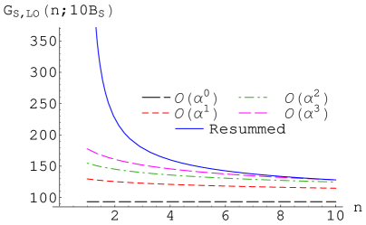
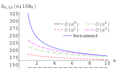
Figure 1: In this plot we show the differences between the expanded and the resummed expression for $G_{(S,P),LO}(n;\mu)$, following the definition given in eq. (29).

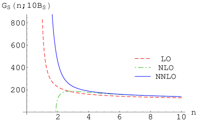
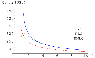
Figure 2: In this plot we show $G_{S}(n;\mu)$ and $G_{P}(n;\mu)$ at different orders in the $1/n$ expansion.

3 Preasymptotic effects in $1/n$ in the ’t Hooft Model

A systematic analysis of the preasymptotic effects in $1/n$ has not been undertaken until the analysis of Ref. [16] and this paper. Therefore, it is interesting to check the methodology in a specific model where the results obtained with the OPE can be tested with the exact results. Here we consider the ’t Hooft model, which will allow us to perform such an analysis. In this model, the preasymptotic corrections to the mass spectrum are known [17] (actually they have a $\ln n$ dependence, which will prove to be crucial) but not those to the decay constants, for which the analysis of the preasymptotic effects in $1/n$ is not an easy issue.

Unlike in the rest of the paper, we will consider the general situation with non-zero (and different) quark masses. We will focus our interest in the scalar and pseudoscalar currents. One reason is that in two dimensions the vector and axial-vector current matrix elements can be related to them. Nevertheless, the main motivation is that we are interested in situations where logarithms of $Q$ can be generated, which can only happen if an infinite number of resonances contributes to the correlator. This does not happen for the vector and axial-vector correlator in the massless limit, where they both become almost trivial, since only one resonance (the ground state) has overlap with the current[29, 30].

3.1 Preasymptotic effects in $1/n$ from the OPE

The main aim here is to repeat up to NLO and in two dimensions the analysis performed in sec. 2. The difference is that now we know the spectrum at NLO, which reads [17]

$$M_{X}^{2}(n)=M^{2}(n)=\sum_{s=-1}^{\infty}B^{(-s)}n^{(-s)}=B^{(1)}n+B^{(0)}+\cdots\,,$$ (32)

and we define $M^{2}_{LO}(n)=B^{(1)}n$. Note that the spectrum is the same for the scalar and pseudoscalar channel. The coefficients $B^{(1)}$ and $B^{(0)}$ are known in the ’t Hooft model. They read [17]

$$B^{(1)}=\pi^{2}\beta^{2}\,,\qquad B^{(0)}=(m_{i,R}^{2}+m_{j,R}^{2})\ln n+{\rm constant}\,,$$ (33)

where $i$ and $j$ represent, respectively, the flavor of the quark and antiquark that make up the meson in the ’t Hooft model, $\beta^{2}=g^{2}N_{c}/(2\pi)$, and $m_{i,R}^{2}=m_{i}^{2}-\beta^{2}$ is the renormalized mass. The explicit expression for the constant term can be found in Ref. [32].

Similarly to the mass we write

$$F_{X}^{2}(n)=F_{X,0}^{2}(n)+\frac{F_{X,1}^{2}(n)}{n}+\dots\,,$$ (34)

and $F_{X,LO}^{2}(n)=F_{X,0}^{2}(n)$, $F_{X,NLO}^{2}(n)=F_{X,0}^{2}(n)+F_{X,1}^{2}(n)/n$. Note that, unlike our former expression for the decay constants, Eq. (12), there is no $n$ multiplying in front. This is due to the fact that in two dimensions the correlator $\Pi_{X}$ goes like

$$\Pi_{X}(q)\sim\ln{\frac{Q^{2}}{\mu^{2}}}\ .$$ (35)

The correlator has also no anomalous dimension in the ’t Hooft model. The definition of the correlators used in this section is the same to the one given in Eq. (1) but with general currents (with in principle different flavours): $J_{S}=\bar{\psi}_{j}\psi_{i}$ and $J_{P}=i\bar{\psi}_{j}\gamma_{5}\psi_{i}$. The hadronic expressions for the correlators read

$$\Pi^{hadr.}_{S} = \sum_{n=1,3,5\dots}^{\infty}\frac{F_{S}^{2}(n)}{M^{2}(n)-q^{2}-i\epsilon}\,,$$ (36)

$$\Pi^{hadr.}_{P} = \sum_{n=0,2,4\dots}^{\infty}\frac{F_{P}^{2}(n)}{M^{2}(n)-q^{2}-i\epsilon}\ ,$$ (37)

where $F_{X}(n)=\langle vac|J_{X}|ij;n\rangle$. We note that only odd and even states contribute to the scalar and pseudoscalar correlator respectively (this implies that for the scalar correlator the ground state does not contribute). This result was obtained in Ref. [29], using some general properties of the ’t Hooft equation operator. Those properties can be understood somewhat on a pure symmetry basis. Nevertheless, it is not an easy task to visualize this symmetry at the Lagrangian level. The situation is similar to the one found in the spectrum of diatomic atoms [33] or of NRQCD in the static limit (see for instance [34]). In those situations a convenient way to deal with the problem is to project the Lagrangian to the Hilbert space sector we are interested in. In our case, this is basically equivalent to ending up in the ’t Hooft equation (wich we present in the next section), where one can use the operator identities found in Ref. [29] for the current matrix elements (however it should also be possible to relate these operator identities with some underlying symmetries of the system), in particular Eq. (51). Using these results one can discriminate which states give non-zero contribution to each correlator.

We now define the Adler-like function in two dimensions

$$\mathcal{A}_{X}\equiv-Q^{2}\frac{d\Pi_{X}(Q^{2})}{dQ^{2}}\ ,$$ (38)

for which its hadronic expressions read

$$\mathcal{A}^{hadr.}_{X}=Q^{2}\sum_{n_{X}}^{\infty}\frac{F_{X}^{2}(n)}{(M(n)^{2}+Q^{2})^{2}}\ ,$$ (39)

where $n_{X}$ stands for the sum for the scalar or pseudoscalar case respectively.

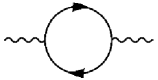
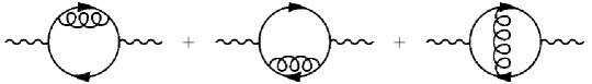
Figure 3: Diagrams that contribute to the OPE at one loop in perturbation theory.

In order to follow the procedure used in the previous section we need the OPE expression for $\mathcal{A}_{X}$. It reads:

$$\mathcal{A}^{pert.}_{X}=\frac{N_{c}}{2\pi}\left(1+\frac{\beta^{2}}{Q^{2}}+D_{X}\frac{m_{i}m_{j}}{Q^{2}}\left(\text{ln}\left(\frac{m_{i}^{2}}{Q^{2}}\right)+\text{ln}\left(\frac{m_{j}^{2}}{Q^{2}}\right)\right)+\frac{2\pi}{N_{c}}D_{X}\frac{m_{j}\langle\bar{\psi}_{i}\psi_{i}\rangle+m_{i}\langle\bar{\psi}_{j}\psi_{j}\rangle}{Q^{2}}\right)$$

$$+\cdots\ ,$$ (40)

where $D_{S}=1$ and $D_{P}=-1$, and we have neglected terms of ${\cal O}(m^{2}/Q^{2})$ (except for the logarithm term) and terms of ${\cal O}(1/Q^{3})$. The pure perturbative piece of this result is obtained from the computation of the diagrams shown in Fig. 3. The condensate contribution is obtained by “collapsing” one of the quark propagators. We see that the coefficient of the quark condensate has no $\ln Q$ piece.

Note that in two dimensions the coupling constant $\beta^{2}$ has dimensions. Therefore, the perturbative and OPE expansions are related. In particular, in two dimensions, there are no problems with renormalons, due to the fact that there are no marginal operators in the Lagrangian.

In Eq. (40) the quark condensate, as usual, only includes the pure non-perturbative contribution, ie. the free result

$$\langle\bar{\psi}_{i}\psi_{i}\rangle_{pert.}=\frac{N_{c}}{2\pi}m_{i}\ln{\frac{m_{i}^{2}}{\mu^{2}}}$$ (41)

has been subtracted and displayed explicitly in $\mathcal{A}^{pert.}_{X}$.

We can now combine all this information with our knowledge of the large $n$ behaviour of the mass spectrum to obtain the $1/n$ preasymptotic effects of the decay constants.

We follow the same procedure of sec. 2.1. To rewrite $\mathcal{A}^{hadr.}_{X}$ using the Euler-Maclaurin formula, we first define $n=2n^{\prime}+1$ for the scalar case and $n=2n^{\prime}$ for the pseudoscalar case, so that we can transform the sums into an integral over a continuous variable. The only term that will give a LO contribution, not suppressed by powers of $Q^{2}$, will be

$$Q^{2}\int_{0}^{\infty}\frac{dn}{2}\frac{F_{X,LO}^{2}(n)}{(M_{LO}^{2}(n)+Q^{2})^{2}}=\int_{0}^{\infty}\frac{dn}{2}\frac{F_{X,0}^{2}(n)}{(n\pi^{2}\beta^{2}+Q^{2})^{2}}=\frac{N_{c}}{2\pi}\ ,$$ (42)

where the last equality is the matching to the partonic result and gives us

$$F_{X,0}^{2}(n)=N_{c}\pi\beta^{2}\ .$$ (43)

In order to go beyond the parton result we need to consider the $1/n$ corrections to the linear behaviour in the mass. Note that the form of the spectrum is different from the one assumed in Ref. [16], or in sec. 2: in the ’t Hooft model we know that $B^{(0)}$ is not a constant and diverges logarithmically in $n$. We actually do not care about the finite piece of $B^{(0)}$, since such contribution would constrain the ${\cal O}(1/n^{2})$ term of the decay constant but not the ${\cal O}(1/n)$ term; this is so because $F^{2}_{X,0}$ is constant. Therefore in what follows we will neglect the constant term in $B^{(0)}$ and only consider the logarithmic correction. Within this approximation, the matching at NLO reads (at logarithmic order, after expanding and integrating by parts),

$$Q^{2}\int_{n^{*}}^{\infty}\frac{dn}{2}\frac{F_{X,1}^{2}(n)/n}{(n\pi^{2}\beta^{2}+Q^{2})^{2}}-Q^{2}\int_{n^{*}}^{\infty}\frac{dn}{2}\frac{F_{X,0}^{2}}{(n\pi^{2}\beta^{2}+Q^{2})^{2}}\frac{(m_{i,R}^{2}+m_{j,R}^{2})}{n\pi^{2}\beta^{2}}$$ (44)

$$\doteq-\frac{N_{c}}{2\pi}\frac{D_{X}}{Q^{2}}\left(2m_{i}m_{j}\right)\text{ln}(Q^{2})\doteq-Q^{2}\int_{n^{*}}^{\infty}\frac{dn}{2}\frac{1}{(n\pi^{2}\beta^{2}+Q^{2})^{2}}N_{c}\pi\beta^{2}\frac{D_{X}(2m_{i}m_{j})}{n\pi^{2}\beta^{2}}\ ,$$

where again $\doteq$ means that the equality is only true at logarithmic order. And so,

$$\frac{F_{X,1}^{2}(n)}{n}=-N_{c}\pi\beta^{2}\frac{2m_{i}m_{j}D_{X}-m_{i,R}^{2}-m_{j,R}^{2}}{n\pi^{2}\beta^{2}}\ .$$ (45)

It will prove useful in the next section to combine the scalar and pseudoscalar result for the decay constant in a single function. We define

$$F^{2}(n)=\,\left\{\begin{array}[]{ll}&F_{S}(n)\,{\rm for}\,n=\,{\rm odd}\\ &F_{P}(n)\,{\rm for}\,n=\,{\rm even}\,.\end{array}\right.$$

Therefore, we have

$$F^{2}(n)=N_{c}\pi\beta^{2}\left[1+\frac{m_{i,R}^{2}+m_{j,R}^{2}}{n\pi^{2}\beta^{2}}+\frac{2m_{i}m_{j}}{n\pi^{2}\beta^{2}}(-1)^{n}\right]\,.$$ (47)

Let us note that there is a term which is sign-alternating.

Finally, we stress that we have obtained these expressions for the decay constant using the OPE, symmetries and the knowledge of the mass spectrum, nothing else. In the next subsection we check whether the explicit numeric computation of the decay constants from the ’t Hooft equation fulfills these expectations.

3.2 Preasymptotic effects in $1/n$ from the hadronic solution

In the ’t Hooft model it is possible to write the decay constants $F_{X}^{2}(n)$ in terms of the light-cone distribution amplitude of the bound state, $\phi^{ij}_{n}(x)$, which is the solution of the equation

$$M^{2}(n)\phi^{ij}_{n}(x)=\left(\frac{m^{2}_{i,R}}{x}+\frac{m^{2}_{j,R}}{1-x}\right)\phi^{ij}_{n}(x)-\beta^{2}\int_{0}^{1}dy\phi^{ij}_{n}(y)\mathrm{P}\frac{1}{(y-x)^{2}}\,,$$ (48)

where $x=p^{+}/P_{n}^{+}$, with $p^{+}$ being the momentum of the quark $i$, and P stands for Cauchy’s Principal Value.

The decay constant for the scalar case then reads [29]

$$F_{S}(n)=\sqrt{\frac{N_{c}}{4\pi}}\int_{0}^{1}dx\phi^{ij}_{n}(x)\left(\frac{m_{i}}{x}-\frac{m_{j}}{1-x}\right)=m_{i}\sqrt{\frac{N_{c}}{\pi}}\int_{0}^{1}dx\frac{\phi^{ij}_{n}(x)}{x}\;\;\text{for $n$ odd}\,,$$ (49)

and zero otherwise. For the pseudoscalar we have

$$F_{P}(n)=\sqrt{\frac{N_{c}}{4\pi}}\int_{0}^{1}dx\phi^{ij}_{n}(x)\left(\frac{m_{i}}{x}+\frac{m_{j}}{1-x}\right)=m_{i}\sqrt{\frac{N_{c}}{\pi}}\int_{0}^{1}dx\frac{\phi^{ij}_{n}(x)}{x}\;\;\text{for $n$ even}\,,$$ (50)

and zero otherwise. Note that in the above two equalities we have used the remarkable identity

$$m_{i}\int_{0}^{1}dx\frac{\phi^{ij}_{n}(x)}{x}=(-1)^{n}m_{j}\int_{0}^{1}dx\frac{\phi^{ij}_{n}(x)}{1-x}\,,$$ (51)

obtained in Ref. [29].

By comparing Eqs. (49) and (50) with Eq. (47) we can obtain expressions for $\int_{0}^{1}dx\frac{\phi^{ij}_{n}(x)}{x}$ with $1/n$ accuracy:

$$\int_{0}^{1}dx\frac{\phi^{ij}_{n}(x)}{x}=\pi\frac{\beta}{m_{i}}\left[1+\frac{m_{i,R}^{2}+m_{j,R}^{2}}{2n\pi^{2}\beta^{2}}+\frac{m_{i}m_{j}}{n\pi^{2}\beta^{2}}(-1)^{n}+{\cal O}\left(\frac{1}{n^{2}}\right)\right]\,.$$ (52)

By using symmetries and the ’t Hooft equation, we can also obtain

$$M^{2}(n)\int_{0}^{1}dx\phi_{n}^{ij}(x) = m_{i}^{2}\int_{0}^{1}dx\frac{\phi^{ij}_{n}(x)}{x}+m_{j}^{2}\int_{0}^{1}dx\frac{\phi^{ij}_{n}(x)}{1-x}$$

$$= \pi{\beta}{m_{i}}\left[1+\frac{m_{i,R}^{2}+m_{j,R}^{2}}{2n\pi^{2}\beta^{2}}+\frac{m_{i}m_{j}}{n\pi^{2}\beta^{2}}(-1)^{n}\right]$$

$$+(-1)^{n}\pi{\beta}{m_{j}}\left[1+\frac{m_{i,R}^{2}+m_{j,R}^{2}}{2n\pi^{2}\beta^{2}}+\frac{m_{i}m_{j}}{n\pi^{2}\beta^{2}}(-1)^{n}\right]+{\cal O}\left(\frac{1}{n^{2}}\right)\,,$$

where in the last equality we have made use of the symmetry property of the ’t Hooft wave functions,

$$\phi^{ij}_{n}(x)=(-1)^{n}\phi^{ji}_{n}(1-x)\ .$$ (54)

These results can also be used to deepen our analytic understanding of the ’t Hooft wave function in the end-point regions in the massless limit (actually we need only one mass to go to zero at each boundary, $m_{i}$ for $x\to 0$, or $m_{j}$ for $x\to 1$). In the massless quark limit the integral in Eq. (52) is dominated by the behaviour of the wave-function in the $x\rightarrow 0$ boundary:

$$\phi^{ij}_{n}(x)=c_{n}x^{\beta_{i}}\left(1+o(x)\right)\ ,$$ (55)

where $\beta_{i}$ is the solution of

$$m_{i,R}^{2}+\beta^{2}\pi\beta_{i}\cot{\pi\beta_{i}}=0\ ,$$ (56)

which in the massless limit approximates to

$$\beta_{i}=\frac{\sqrt{3}}{\pi}\frac{m_{i}}{\beta}+o(m_{i})\,.$$ (57)

Therefore we obtain for the integral

$$\lim_{m_{i}\rightarrow 0}m_{i}\int_{0}^{1}dx\frac{\phi^{ij}_{n}(x)}{x}=c_{n}\frac{\pi\beta}{\sqrt{3}}\,,$$ (58)

and, in the massless quark limit, the problem of getting the decay constants could be reformulated as that of obtaining the coefficient $c_{n}$. One can find its value for $n=0$ (note that this result does also require $m_{j}=0$):

$$\lim_{m_{i,j}\rightarrow 0}c_{0}=1.$$ (59)

In principle, there are several ways to obtain this result. One can work along the lines of Ref. [36] to obtain an approximated Schrodinger-like equation, which can be approximately solved for the ground state. Another possibility to fix the value $c_{0}$ is by matching the solution $\phi_{0}=1$ (the exact solution in the strict massless limit) and the solution $\phi_{0}=c_{0}x^{\beta_{i}}$ in the region of overlap (the latter is valid for $x\ll 1$, whereas it can be approximated to a constant, $c_{0}$, for values larger than $e^{-\beta/m_{i}}$, which is a very small quantity for small masses. Therefore, there is a region on which the $constant$ solutions: “$c_{0}$”, and “1”, overlap and should be equal by continuity). One can also use the value of $\lim_{m_{i}\rightarrow 0}\int_{0}^{1}\phi_{0}(x)=1$, to fix $c_{0}$.

Nevertheless, in this paper, we are mainly interested in the study of high excitations. The combination of Eq. (58) and Eq. (47) allows us to give the following prediction for $c_{n}$:

$$\lim_{m_{i}\rightarrow 0}c_{n}=\sqrt{3}\left(1-\frac{1}{\pi^{2}}\frac{1}{n}+\frac{m_{j}^{2}}{2n\pi^{2}\beta^{2}}+{\cal O}(1/n^{2})\right)\,.$$ (60)

How much of all this can be understood by a direct analytic computation? In principle the ’t Hooft equation can only be solved numerically. Nevertheless, for large $n$, the ’t Hooft equation can be approximated by the boundary-layer equation [30]:

$$\phi^{i}(\xi)=\frac{m^{2}_{i,R}}{\xi}\phi^{i}(\xi)-\beta^{2}\int_{0}^{\infty}d\xi^{\prime}\phi^{i}(\xi^{\prime})\mathrm{P}\frac{1}{(\xi^{\prime}-\xi)^{2}}\,,$$ (61)

where

$$\phi^{i}(\xi)\equiv\lim_{n\rightarrow\infty}\phi^{ij}_{n}(\xi/M^{2}(n))\,,$$ (62)

as far as we are not in the $x\rightarrow 1$ limit (one could also write a symmetric equation convenient for $x\sim 1$ region). It is possible to analytically solve the Mellin transform of this equation [32]. In particular, one obtains

$$\int_{0}^{\infty}d\xi\frac{\phi^{i}(\xi)}{\xi}=\pi\frac{\beta}{m_{i}}\,,\qquad\int_{0}^{\infty}d\xi\phi^{i}(\xi)=\pi\frac{m_{i}}{\beta}\ .$$ (63)

From these results one easily checks the leading order terms of Eqs. (52) and Eq. (60). Note that for the last equation $\phi_{n}(x)\simeq c_{n}x^{\beta_{i}}$ is valid for $x\ll 1$. In particular, for high excitations, the region of validity of this expression is very small, restricted to the region $\xi\equiv M_{n}^{2}x\ll\beta^{2}$.

In order to check the $1/n$ corrections in Eqs. (52) and (60), one should be able to go one order beyond the analysis of Ref. [32], which appears to be a formidable task. This would go far beyond the aim of this paper. Instead, in the remainder of this section, we will try to see whether Eqs. (52), (59) and (60) can be confirmed by a direct numerical computation.

In order to perform the numerical analysis we will use two methods:

1. One is based on the Brower-Spence-Weis improvement of the Multhopp technique [32]. In this method the ’t Hooft wave function is decomposed in a basis of sin functions. Therefore, the ’t Hooft equation becomes a infinity-dimensional matrix, which at the numerical level is truncated for a finite number of sines. This method appears to be very well suited for very high excitations, and allows us to work with different quark masses without problems. Nevertheless, it has some problems for very low masses and it does not have the right functional behaviour in the $x\rightarrow 0,1$ limit.

2. The other method that we use is based on the decomposition of the ’t Hooft wave function in a basis of $x^{\beta_{i}}(1-x)^{\beta_{j}}P(x)$ functions, where $P(x)$ are Jacobi polynomials. This method has already been used in Refs. [37, 38]. Unfortunately, we are only able to give reliable numbers for even states with equal masses. For those states we can perform numerical checks with the numbers given in [38] (we use them as numerical check of our implementation of the method, since our interest is on a different regime than that of [38]: high excitations and small masses). In any case, this method does not appear to work very well for very high excitations, as well as for very small masses (though it can reach lower limits than method 1). Moreover, at a certain point the introduction of more Jacobi polynomials in the calculation spoils the convergence of the result, except for the wave function of the ground state. On the other hand, by construction, this method should have the right functional behaviour in the $x\rightarrow 0,1$ limit.

We now first try to check Eq. (52). In Fig. 4 we show our results with method 2. The results from the numerical calculation are presented with some rough estimation of their uncertainty, performed by considering the difference between evaluating directly Eq. (52) or a properly weighted (see tables 2 and 3 for the definition) combination of Eq. (3.2). We show in tables 2 and 3 the differences for two mass values. With this method we cannot go to very large values of $n$, nor consider different quark masses or odd values of $n$. Nevertheless, for the range of values one can consider with this method the agreement is perfect. The $1/n$ and mass dependence can be unambiguously checked very nicely.

$$\begin{array}[]{clclclc}\hline\cr n&\vline&\frac{m_{i}}{\beta}\int dx\frac{\phi_{n}(x)}{x}&\vline&\frac{M^{2}(n)}{2m_{i}\beta}\int dx\phi_{n}(x)\\ \hline\cr 2&\vline&3.24&\vline&3.24\\ \hline\cr 4&\vline&3.20&\vline&3.20\\ \hline\cr 6&\vline&3.19&\vline&3.18\\ \hline\cr\end{array}$$

Table 2: Results from the numerical calculation using method 2 for $m_{i}=m_{j}=\beta$.

$$\begin{array}[]{clclclcc}\hline\cr n&\vline&\frac{m_{i}}{\beta}\int dx\frac{\phi_{n}(x)}{x}&\vline&\frac{M^{2}(n)}{2m_{i}\beta}\int dx\phi_{n}(x)\\ \hline\cr 2&\vline&2.97&\vline&2.96\\ \hline\cr 4&\vline&3.06&\vline&3.05\\ \hline\cr 6&\vline&3.10&\vline&3.08\\ \hline\cr\end{array}$$

Table 3: Results from the numerical calculation using method 2 for $m_{i}=m_{j}=0.1\beta$.

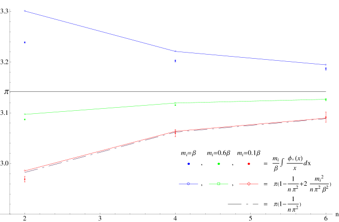
Figure 4: In this plot we show our results for Eq. (52) with method 2. The bands reflect the difference between using directly Eq. (52) or a properly weighted combination of Eq. (3.2), which we show in tables 2 and 3.

In Fig. 5 we show our results with method 1. In this case we can take much larger values of $n$, although not so small quark masses as in method 2. On the other hand, in this case, the use of Eq. (52) or the properly weighted combination of Eq. (3.2) is basically indistinguishable. We can see clearly in this figure that scalar and pseudoscalar states follow different curves, as their corrections involve the difference of the masses of the quarks or their addition, respectively. The behaviour of the corrections changes from increasing to decreasing with $n$ depending on how the sum and the difference of the quark masses compare to $2\beta$. We can also see how the numerical results approach the expected analytic expressions as $n$ increases.

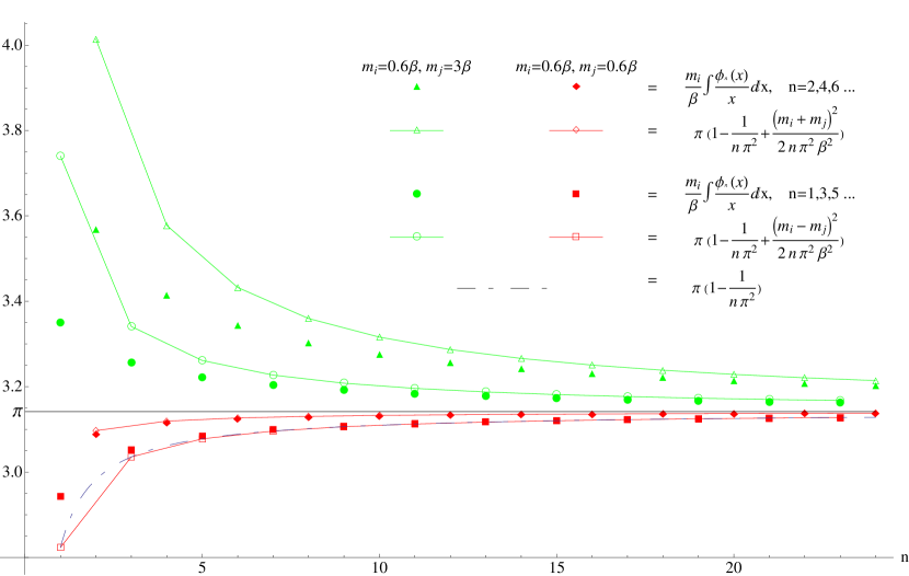
Figure 5: In this plot we show our results with method 1 for Eq. (52).

We conclude that we have been able to unambiguously and nicely check Eqs. (52) and (3.2) numerically. We note that we have been able to visualize the mass dependence and the sign alternating terms, and that, in particular, we are reaching a numerical precision below 1%.

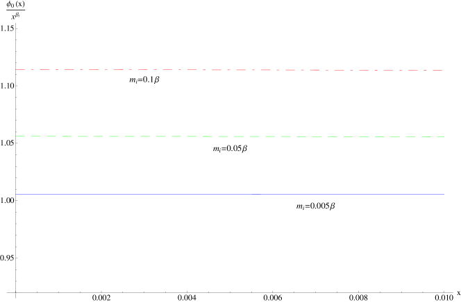
Figure 6: In this plot we show our results with method 2 for Eq. (59) with $m_{i}=m_{j}$. Due to the small values of the quark masses, in the range we are showing the functions are essentially constant.

We now try to check Eq. (59). In Fig. 6 we show the plot of $\phi_{0}(x)/x^{\beta_{i}}$ for small values of $x$ calculated with method 2, and we can see that, indeed, as we approach the massless limit $c_{0}$ tends to $1$. Method 1 is not efficient for the evaluation of the wave function near the origin, for, as we said before, it does not have the right functional behaviour in the $x\to 0,\,1$ limit: it yields a sinusoidal function that oscillates around the right solution, until we approach the boundaries, where the curve that the oscillations follow does not die off as it should.

Finally, we try to check Eq. (60). In this case we cannot use method 2: although it incorporates by definition the right $c_{n}x^{\beta_{i}}$ behaviour, its numerical precision at high values of $n$ is very poor. We are left then with method 1. Numerical precision in this case is not so much of an issue, but due to the aforementioned limitations of this method we can only hope to get some estimate for $c_{n}$ by finding the path around which our sinusoidal solutions oscillate when $x$ is not too close to $0$, and then extrapolate this path to the limit $x\to 0$. In figure 7 we show our results for n=4 with $m_{i}=0.001\beta$, $m_{j}=2\beta$: we evaluate $\phi_{4}(x)/x^{\beta_{i}}$ at points separated a distance $\Delta x=10^{-6}$, starting at $x=10^{-5}$ and ending at $x=10^{-3}$, and we fit them to a quadratic function. Depending on how many of the points that are closer to the origin we include in the fit, the resulting curve will be one or another, as shown in the plot, somewhat oscillating around the two extreme curves displayed. The possible values of the fit at $x=0$ are the possible values of $c_{4}$ that we can find with method 1. In figure 8 we show the results up to $n=25$ for the cases $m_{i}=0.001\beta$, $m_{j}=2\beta$ and $m_{i}=0.001\beta$, $m_{j}=0.001\beta$. Overall, this numerical analysis serves as a consistency check of Eq. (60).

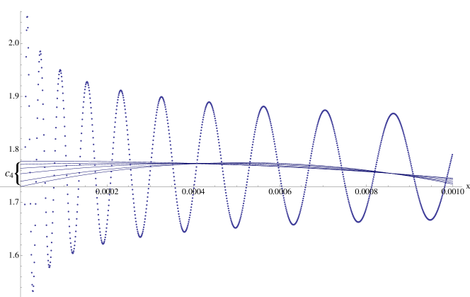
Figure 7: The dots in this plot correspond to values of $\phi_{4}(x)/x^{\beta_{i}}$ sampled with $\Delta x=10^{-6}$ for $m_{i}=0.001\beta$, $m_{j}=2\beta$. We show some of the possible fits to a quadratic function, depending on the set of points used, from all those that fall within the interval $x\in[10^{-5},10^{-3}]$ to only those that are within $x\in[10^{-4},10^{-3}]$. The possible values of the fits at the origin give us an estimated range for $c_{4}$.

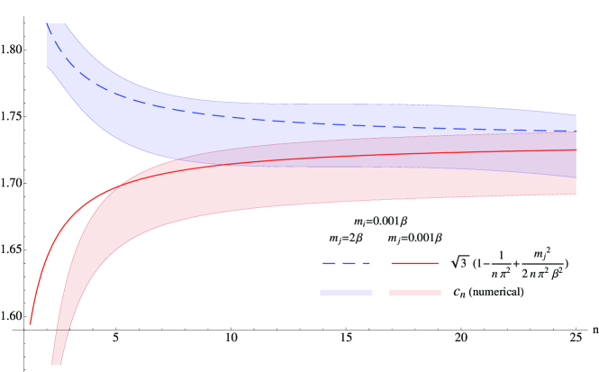
Figure 8: In this plot we show our results with method 1 for Eq. (60).

4 Finite $N_{c}$

This far the discussion has been restricted to the large $N_{c}$ limit. We would like to finish this paper by studying models valid at finite $N_{c}$. One model with the right analytic properties for the current-current correlator and with the correct limit in the large $N_{c}$ limit has been built in Ref. [2]. This model is also able to reproduce the leading parton-model logarithm at large $Q^{2}$. Working analogously to previous sections, we will consider whether subleading perturbative corrections can be incorporated in this model, and see if by including $1/N_{c}$ effects there appears any connection between the slopes of resonances of different parity. For definiteness, we will consider the vector-vector correlator but most of the discussion trivially applies to any other current-current correlator; in particular the scalar or pseudoscalar correlator, for which the only complication would be to take into account the anomalous dimensions. Therefore, we take

$$\Pi_{V}^{\mu\nu}(q)\equiv(q^{\mu}q^{\nu}-g^{\mu\nu}q^{2})\Pi_{V}(q)\equiv i\int d^{4}xe^{iqx}\langle vac|J_{V}^{\mu}(x)J_{V}^{\nu}(0)|vac\rangle\,,$$ (64)

where $J_{V}^{\mu}=\sum_{f}Q_{f}\bar{\psi}_{f}\gamma^{\mu}\psi_{f}$. In order to avoid divergences, we will work with the Adler function

$${\cal A}_{V}(Q^{2})\equiv-Q^{2}{d\over dQ^{2}}\Pi_{V}(Q^{2})=Q^{2}\int_{0}^{\infty}dt\frac{1}{(t+Q^{2})^{2}}\frac{1}{\pi}\text{Im}\Pi_{V}(t)\,.$$ (65)

We consider the following expression for the vacuum polarization,

$$\Pi_{V}(Q^{2})=\sum_{n=0}^{\infty}{F_{V}^{2}(n)\over\left(\frac{Q^{2}}{\Lambda^{2}}\right)^{1-\frac{C}{\pi N_{c}}}\Lambda^{2}+M_{V}^{2}(n)}\,.$$ (66)

For $F_{V}^{2}(n)=$constant and $M_{V}^{2}(n)=B_{V}n$, we recover the model of Ref. [2]. Here we will allow $F_{V}^{2}(n)$ to be $n$-dependent. The Adler function for this model reads

$${\cal A}_{V}(Q^{2})=(1-\frac{C}{\pi N_{c}})z\sum_{n=0}^{\infty}\frac{F_{V}^{2}(n)}{\Lambda^{2}}\frac{1}{(z+n)^{2}}\,,\qquad z=\left(\frac{Q^{2}}{\Lambda^{2}}\right)^{1-\frac{C}{\pi N_{c}}}\ .$$ (67)

For simplicity we will set $\Lambda^{2}=B_{V}$ in the following. It will also be enough for our purposes to keep the analysis of ${\cal A}(Q^{2})$ to the lowest order in the OPE. Therefore, we only consider

$${\cal A}_{V,pert.}(Q^{2})={\cal A}_{0}\left(1+c_{1}\frac{\alpha_{\cal A}(Q^{2})}{\pi}\right)=-Q^{2}{d\over dQ^{2}}{\cal A}_{0}\int_{0}^{\infty}dt\frac{1}{(t+Q^{2})^{2}}\left(1+c_{1}\frac{\alpha_{M}(t)}{\pi}\right)\,,$$ (68)

where $\alpha_{\cal A}(Q^{2})$ and $\alpha_{M}(t^{2})$ admit an analytic expansion in terms of $\alpha_{\rm s}(Q^{2})$ (computed in the $\overline{\rm MS}$ scheme):

$$\alpha_{\cal A}(Q^{2}) = \alpha_{\rm s}(Q^{2})\left(1+\frac{c_{2}}{c_{1}}\frac{\alpha_{\rm s}(Q^{2})}{\pi}+\frac{d_{3}}{c_{1}}\frac{\alpha_{\rm s}^{2}(Q^{2})}{\pi^{2}}+\cdots\right)$$ (69)

$$\alpha_{M}(t) = \alpha_{\rm s}(t)\left(1+\frac{c_{2}}{c_{1}}\frac{\alpha_{\rm s}(t)}{\pi}+\frac{c_{3}}{c_{1}}\frac{\alpha_{\rm s}^{2}(t)}{\pi^{2}}+\cdots\right)\ .$$ (70)

The coefficients $c_{i}$ and $d_{i}$ have been computed in Ref. [26] (they can be obtained from each other through dispersion relations):

$$c_{1} = \frac{3N_{c}}{8}$$ (71)

$$c_{2} = \frac{N_{c}^{2}}{128}\left((243-176\zeta(3))-\frac{4n_{f}}{N_{c}}(11-8\zeta(3))\right)$$

$$c_{3} = \frac{N_{c}^{3}}{27648}\left[346201-2904\pi^{2}-324528\zeta(3)+63360\zeta(5)\right.$$

$$\left.+\frac{2n_{f}}{N_{c}}(-62863+528\pi^{2}+51216\zeta(3)-5760\zeta(5))\right]+\frac{\left(\sum_{f}Q_{f}\right)^{2}}{\sum_{f}Q_{f}^{2}}\frac{N_{c}^{2}}{1024}\left(\frac{176}{3}-128\zeta(3)\right)\ ,$$

and

$${\cal A}_{0}=\sum_{f}Q_{f}^{2}\frac{4}{3}\frac{N_{c}}{16\pi^{2}}\ .$$

As before, through the Euler-Maclaurin formula we can see that the matching between the perturbative and the hadronic calculations at logarithmic order requires that

$${\cal A}_{0}\left(1+c_{1}\frac{\alpha_{\cal A}(Q^{2})}{\pi}\right)=\left(1-\frac{C}{\pi N_{c}}\right)z\int_{0}^{\infty}dn\frac{F_{V,0}^{2}(n)}{B_{V}}\frac{1}{(z+n)^{2}}\ ,$$ (72)

where we have added the subscript $0$ to $F_{V}^{2}(n)$, in agreement with our notation of sec. 2.1. In Ref. [16], we obtained that

$$\frac{F_{V,0}^{2,\infty}}{B_{V}}={\cal A}_{0}\left(1+c_{1}^{\infty}\frac{\alpha^{\infty}_{M}(B_{V}n)}{\pi}\right)\ ,$$ (73)

where the upperscript $\infty$ stands for the $N_{c}\rightarrow\infty$ limit. One could consider that the same structure should hold for finite $N_{c}$ in our model and that the decay constant should then be proportional to $1+c_{1}\frac{\alpha_{M}(B_{V}n)}{\pi}$. However, this is not so due to the specific functionality on $Q^{2}$ that we have introduced. For instance, it is interesting to consider the following quantity

$$z\int_{0}^{\infty}dn\frac{1}{(n+z)^{2}}\alpha_{M}(B_{V}n)=\alpha_{\cal A}(B_{V}z)=\alpha_{\cal A}(Q^{2})-\frac{C}{\pi N_{c}}\ln\frac{Q^{2}}{B_{V}}\beta_{\cal A}^{\infty}(\alpha_{\cal A}^{\infty}(Q^{2}))+O(\frac{1}{N_{c}^{2}})\ .$$ (74)

The first term is what we should obtain to match the perturbative calculation. If we want $F_{V,0}^{2}(n)$ to be expressed in terms of $\alpha_{\rm s}(B_{V}n)$ we have to fine tune it in order to eliminate the second extra term.

If we write

$$\frac{F_{V,0}^{2}}{B_{V}}=\frac{{\cal A}_{0}}{1-\frac{C}{\pi N_{c}}}\left(1+c_{1}\frac{\alpha_{M}(B_{V}n)}{\pi}\right)+\frac{C}{\pi N_{c}}\frac{\delta F_{V,0}^{2}}{B_{V}}\ ,$$ (75)

the following equality has to be satisfied (here, with the precision of the calculation, we can replace $z\simeq Q^{2}/B_{V}$)

$$z\int_{0}^{\infty}dn\frac{1}{(n+z)^{2}}\frac{\delta F_{V,0}^{2}}{B_{V}}=\ln\frac{Q^{2}}{B_{V}}\beta_{\cal A}^{\infty}(\alpha_{\cal A}^{\infty}(Q^{2}))\ .$$ (76)

This implies that $\delta F^{2}\sim\alpha_{\rm s}^{2}(B_{V})\ln n$. Note that $\beta_{0}$ and $\beta_{1}$ are the same for $\alpha_{\cal A}$, $\alpha_{M}$ and $\alpha_{\rm s}$. Therefore, at low orders in $\alpha$ the distinction between different renormalization schemes is superfluous.

We can try to refine our ansatz. If we rewrite the expression for $F_{V}^{2}$ in the following way,

$$\frac{F_{V,0}^{2}}{B_{V}} = \frac{{\cal A}_{0}}{1-\frac{C}{\pi N_{c}}}\left[\left(1+c_{1}\frac{\alpha_{M}(B_{V}n^{1+\frac{C}{\pi N_{c}}})}{\pi}\right)+\frac{C}{\pi N_{c}}\frac{\delta{\tilde{F}}_{V,0}^{2}}{B_{V}}\right]$$

$$= \frac{{\cal A}_{0}}{1-\frac{C}{\pi N_{c}}}\left[\left(1+c_{1}\frac{\alpha_{M}(B_{V}n)}{\pi}+\frac{c_{1}}{\pi}\frac{C}{\pi N_{c}}\ln n\beta_{M}^{\infty}(\alpha_{M}^{\infty}(B_{V}n))+O(\frac{1}{N_{c}^{2}})\right)+\frac{C}{\pi N_{c}}\frac{\delta{\tilde{F}}_{V,0}^{2}}{B_{V}}\right]\ ,$$

some logs are reabsorbed in $\alpha_{M}(B_{V}n^{1+\frac{C}{\pi N_{c}}})$ and $\delta{\tilde{F}}_{V,0}^{2}\sim{\cal O}(\alpha_{\rm s}^{3}(B_{V}),\alpha_{\rm s}^{3+s}(B_{V})\ln^{s}n)$. We can easily obtain the coefficient multiplying $\alpha_{\rm s}^{3}(B_{V})$. We find that, at $\mathcal{O}(\alpha_{\rm s}^{3})$,

$$\frac{\delta{\tilde{F}}_{V,0}^{2}}{B_{V}}=-\frac{2}{3\pi}\beta_{0}^{2}c_{1}\alpha_{\rm s}(B_{V})^{3}\ .$$ (78)

The calculations for the axial-vector case are equal replacing $B_{V}$ by $B_{A}$ (the slope of the Regge trajectory in the axial-vector case). Therefore, as in Ref. [16], we can satisfy the constraints of the OPE with independent values for $B_{V}$ and $B_{A}$. Thus, we conclude that the OPE cannot constrain $B_{V}$ and $B_{A}$ to be equal for general models with the right analytic properties at finite $N_{c}$. Note as well that, in general, at finite $N_{c}$

$$\frac{F_{V,0}^{2}(n)}{|dM_{V,LO}^{2}(n)/dn|}\not=\frac{1}{\pi}{\rm Im}\Pi^{pt.}_{V}(M_{V,LO}^{2}(n))\,.$$ (79)

4.1 $\rho$ at finite $N_{c}$

We now briefly consider what this model tells us about the computation of $\rho(t)\equiv\frac{1}{\pi}{\rm Im}\Pi_{V}(t)$. This is a physical observable related with $\sigma(e^{+}e^{-}\rightarrow{\rm hadrons})$.

We first note that one can approximate the sum over $n$ by an integral (i.e. use the Euler McLaurin expansion) if $q^{2}\rightarrow\infty$ and $|\arg z|<\pi$ for the model of Ref. [2]. At this respect the modification to this model introduced by us is simply the introduction of logs of $n$ in the decay constants, which should not change the analytic properties of the function. This allows us to obtain the OPE expression for the vacuum polarization from the hadronic expression if $|\arg z|<\pi$, as in the original model of Ref. [2]. For $q^{2}$ positive we do have $|\arg z|<\pi$. Thus, we can find the OPE expression from the hadronic one, and vice versa, obtain the hadronic expression from the OPE. In particular, we can obtain its imaginary part, which corresponds to $\rho(t)$. Part of the original structure of $\rho(s)$ will be lost in the way, as the OPE misses non-analytic terms. The associated error is exponential with an exponent that vanishes when $n_{f}\rightarrow 0$ (leaving aside the fact that one expects the series to be asymptotic). Therefore, the general structure of the solution would be

$$\rho(s)=\rho_{pert.}(s)+({\rm power\ like})+({\rm exp.\;suppr.})\,,$$

where only the last term does not follow from the OPE. Unfortunately this result has been obtained for an specific model. In general, one cannot get in a model independent way that

$$\rho(s)=\rho_{pert.}(s)+\cdots\,,$$

where the dots mean a contribution that decays to zero faster than any power of $1/\ln s$.

5 Conclusions

We have studied the constraints that the OPE imposes on models for current-current correlators inspired in the large $N_{c}$ limit and Regge trajectories. We have considered the case of scalar/pseudoscalar correlators. Assuming a model for the mass spectrum consisting of a linear Regge behaviour plus corrections in $1/n$, we have obtained the logarithmic behaviour in $n$ of the decay constants within a systematic expansion in $1/n$. We have accomplished this by matching the hadronic and OPE expressions of the Adler function. The inclusion of $1/n$ corrections to the decay constants is compulsory if one aims at going beyond the leading partonic result, as the $1/n$ terms are needed to produce logarithms of $Q^{2}$ in the Euclidean. We have performed a numerical analysis of our results, in which we have seen the importance of the resummation of the $\ln n$ terms of the decay constants, specially for low $n$. Our results show that it is possible to have a different slope, $B_{S/P}$, for the Regge behaviour of the scalar and pseudoscalar spectrum, and yet comply with all the constraints imposed by the OPE (including perturbative corrections).

In order to check our setup in a controlled environment, where the results obtained with the OPE can be tested with the exact results, we have studied the preasymptotic effects of the scalar/pseudoscalar correlators in the ’t Hooft model (QCD in 2 dimensions in the large $N_{c}$ limit). This has allowed us to compute the $1/n$ corrections to the decay constants in the ’t Hooft model for the first time. Actually, the connection between the OPE and the decay constants provides us with a relatively easy way of finding $1/n$ corrections to hadronic matrix elements in the ’t Hooft model. A direct analytic computation from the ’t Hooft equation appears to be quite involved, however we have been able to confirm our results with the numerical evaluation from the ’t Hooft equation.

Finally, we have also considered a model at finite $N_{c}$ [2] and modified it to allow for the inclusion of perturbative (logarithmic) corrections. We have then obtained the associated decay constants that are consistent with perturbation theory, though they are no longer trivially related with the perturbative expression of the imaginary part of the correlator. We have seen that consistency of this model with the OPE can be obtained with different slopes for the Regge trajectory associated to each channel.

Acknowledgments. This work is partially supported by the network Flavianet MRTN-CT-2006-035482, by the spanish grant FPA2007-60275, by the Spanish Consolider-Ingenio 2010 Programme CPAN (CSD2007-00042), and by the catalan grant SGR2005-00916.

Appendix A Appendix

In this appendix we will present general, model-independent, matching formulas between the OPE and the hadronic calculation both for vector/axial-vector (for the notation in this case, see Ref. [16]) and for scalar/pseudo-scalar correlators, within an expansion in powers of $1/M_{n}^{2}$.

The procedure is the same as in the main body of the text. Take the Adler function ($\mathcal{A}_{X}$ in the vector/axial-vector case, $\mathcal{B}_{X}$ in the scalar/pseudo-scalar case), transform it using the Euler-Maclaurin formula, and focus on the piece that can produce logarithms, namely, the integral.

A.1 Vector/Axial-vector correlators

In this case we work with

$$Q^{2}\int_{n^{*}}^{\infty}dn\frac{F^{2}_{X}(n)}{(Q^{2}+M_{n}^{2})^{2}}=Q^{2}\int_{M_{n^{*}}^{2}}^{\infty}dM_{n}^{2}\frac{1}{\left|\frac{dM_{n}^{2}}{dn}\right|}\frac{F^{2}_{X}(n)}{(Q^{2}+M_{n}^{2})^{2}}\ .$$ (80)

Now, instead of assuming a model for $M_{n}$, we will just expand

$$\frac{1}{\left|\frac{dM_{n}^{2}}{dn}\right|}F^{2}_{X}(n)\equiv\widetilde{F}_{X,0}(M_{n}^{2})+\frac{\widetilde{F}_{X,1}(M_{n}^{2})}{M_{n}^{2}}+\frac{\widetilde{F}_{X,2}(M_{n}^{2})}{M_{n}^{4}}+\dots$$ (81)

Within this expansion, retracing the steps of section 3 in Ref. [16] the matching conditions between OPE and hadronic calculations are trivially obtained:

• LO: $\widetilde{F}_{0,X}(M_{n}^{2})=\text{\Large{$\frac{1}{\pi}$}}\text{Im}\Pi^{pt.}_{X}(M_{n}^{2})$

• NLO: $\widetilde{F}_{1,X}(M_{n}^{2})=0$

• NNLO: $\widetilde{F}_{2,X}(M_{n}^{2})=\text{\Large{$\frac{35}{968\pi^{2}}$}}\beta_{0}N_{c}^{2}\alpha_{\rm s}^{2}(M_{n}^{2})\text{\Large{$\frac{\beta(\alpha_{\rm s}(\mu))\langle vac|G^{2}(\mu)|vac\rangle}{N_{c}^{2}}$}}\ .$

A.2 Scalar/Pseudo-scalar correlators

Here we work with

$$Q^{4}\int_{n^{*}}^{\infty}dn\frac{F^{2}_{X}(n)}{(Q^{2}+M_{n}^{2})^{3}}=Q^{4}\int_{M_{n^{*}}^{2}}^{\infty}dM_{n}^{2}\frac{1}{\left|\frac{dM_{n}^{2}}{dn}\right|}\frac{F^{2}_{X}(n;\mu)}{(Q^{2}+M_{n}^{2})^{3}}\ .$$ (82)

As the dimensions of these correlators are different from those of the vector/axial-vector correlators, we will use a different expansion,

$$\frac{1}{\left|\frac{dM_{n}^{2}}{dn}\right|}F^{2}_{X}(n;\mu)\equiv M_{n}^{2}\left(\bar{F}_{X,0}(M_{n}^{2};\mu)+\frac{\bar{F}_{X,1}(M_{n}^{2};\mu)}{M_{n}^{2}}+\frac{\bar{F}_{X,2}(M_{n}^{2};\mu)}{M_{n}^{4}}+\dots\right)\ .$$ (83)

And the matching results are

• LO: $\bar{F}_{0,X}(M_{n}^{2};\mu)=\text{\Large{$\frac{1}{M_{n}^{2}}\frac{1}{\pi}$}}\text{Im}\Pi^{pt.}_{X}(M_{n}^{2};\mu)$

• NLO: $\bar{F}_{1,X}(M_{n}^{2};\mu)=0$

• NNLO: $\bar{F}_{2,X}(M_{n}^{2};\mu)=\text{\Large{$\frac{3}{11\pi}$}}\beta_{0}\bar{\gamma_{0}}\text{\large{$\left(\frac{\alpha_{\rm s}(M_{n}^{2})}{\alpha_{\rm s}(\mu^{2})}\right)^{2\bar{\gamma_{0}}}$}}N_{c}\alpha_{\rm s}(M_{n}^{2})\text{\Large{$\frac{\beta(\alpha_{\rm s}(\mu))\langle vac|G^{2}(\mu)|vac\rangle}{N_{c}^{2}}$}}$  .

References

- [1] M. A. Shifman, A. I. Vainshtein and V. I. Zakharov, Nucl. Phys. B 147, 385 (1979).
- [2] B. Blok, M. A. Shifman and D. X. Zhang, Phys. Rev. D 57, 2691 (1998) [Erratum-ibid. D 59, 019901 (1999)] [arXiv:hep-ph/9709333].
- [3] M. A. Shifman, arXiv:hep-ph/0009131.
- [4] S. R. Beane, Phys. Rev. D 64, 116010 (2001) [arXiv:hep-ph/0106022].
- [5] M. Golterman, S. Peris, B. Phily and E. De Rafael, JHEP 0201, 024 (2002) [arXiv:hep-ph/0112042].
- [6] T. D. Cohen and L. Y. Glozman, Int. J. Mod. Phys. A 17, 1327 (2002) [arXiv:hep-ph/0201242].
- [7] M. Golterman and S. Peris, Phys. Rev. D 67, 096001 (2003) [arXiv:hep-ph/0207060].
- [8] S. S. Afonin, A. A. Andrianov, V. A. Andrianov and D. Espriu, JHEP 0404, 039 (2004) [arXiv:hep-ph/0403268].
- [9] J. J. Sanz-Cillero, Nucl. Phys. B 732, 136 (2006) [arXiv:hep-ph/0507186].
- [10] M. Shifman, arXiv:hep-ph/0507246.
- [11] O. Cata, M. Golterman and S. Peris, Phys. Rev. D 74, 016001 (2006) [arXiv:hep-ph/0602194].
- [12] S. S. Afonin and D. Espriu, JHEP 0609, 047 (2006) [arXiv:hep-ph/0602219].
- [13] M. Golterman and S. Peris, Phys. Rev. D 74, 096002 (2006) [arXiv:hep-ph/0607152].
- [14] M. Jamin and V. Mateu, arXiv:0802.2669 [hep-ph].
- [15] G. ’t Hooft, Nucl. Phys. B 72, 461 (1974).
- [16] J. Mondejar and A. Pineda, JHEP 0710, 061 (2007) [arXiv:0704.1417 [hep-ph]].
- [17] G. ’t Hooft, Nucl. Phys. B 75, 461 (1974).
- [18] J. Mondejar, A. Pineda and J. Rojo, JHEP 0609, 060 (2006) [arXiv:hep-ph/0605248].
- [19] J. Mondejar and A. Pineda, work in progress.
- [20] K. G. Chetyrkin, Phys. Lett. B 390, 309 (1997) [arXiv:hep-ph/9608318].
- [21] P. A. Baikov, K. G. Chetyrkin and J. H. Kuhn, Phys. Rev. Lett. 96, 012003 (2006) [arXiv:hep-ph/0511063].
- [22] L. R. Surguladze and F. V. Tkachov, Nucl. Phys. B 331, 35 (1990).
- [23] F. Campanario and A. Pineda, Phys. Rev. D 72, 056008 (2005) [arXiv:hep-ph/0508217].
- [24] R. Tarrach, Nucl. Phys. B 183, 384 (1981).
- [25] K. G. Chetyrkin, Phys. Lett. B 404, 161 (1997) [arXiv:hep-ph/9703278].
- [26] S. G. Gorishnii, A. L. Kataev and S. A. Larin, Phys. Lett. B 259, 144 (1991); L. R. Surguladze and M. A. Samuel, Phys. Rev. Lett. 66, 560 (1991) [Erratum-ibid. 66, 2416 (1991)]; K. G. Chetyrkin, Phys. Lett. B 391, 402 (1996) [arXiv:hep-ph/9608480].
- [27] W. M. Yao et al. [Particle Data Group], J. Phys. G 33, 1 (2006).
- [28] A. V. Anisovich et al., Phys. Lett. B 517, 261 (2001).
- [29] C. G. Callan, N. Coote and D. J. Gross, Phys. Rev. D 13, 1649 (1976).
- [30] M. B. Einhorn, Phys. Rev. D 14, 3451 (1976).
- [31] A. R. Zhitnitsky, Phys. Lett. B 165, 405 (1985) [Sov. J. Nucl. Phys. 43, 999.1986 YAFIA,43,1553 (1986 YAFIA,43,1553-1563.1986)].
- [32] R. C. Brower, W. L. Spence and J. H. Weis, Phys. Rev. D 19, 3024 (1979).
- [33] A. Messiah, “Quantum Mechanics. Vol. 2 (German Translation),” De Gruyter/berlin 1979, 585p
- [34] N. Brambilla, A. Pineda, J. Soto and A. Vairo, Rev. Mod. Phys. 77, 1423 (2005) [arXiv:hep-ph/0410047].
- [35] M. Burkardt, Phys. Rev. D 53, 933 (1996) [arXiv:hep-ph/9509226].
- [36] G. ’t Hooft at the New Phenomena in Subnuclear Physics Part A, Ed. A. Zichini, 1977 (Proceedings of the International School in Subnuclear Physics, Erice, 1975).
- [37] W. A. Bardeen, R. B. Pearson and E. Rabinovici, Phys. Rev. D 21, 1037 (1980).
- [38] P. Ditsas and G. Shaw, Nucl. Phys. B 229, 29 (1983).