The solar photospheric abundance of hafnium and thorium.

Abstract

Context. The stable element hafnium (Hf) and the radioactive element thorium (Th) were recently suggested as a suitable pair for radioactive dating of stars. The applicability of this elemental pair needs to be established for stellar spectroscopy.

Aims. We aim at a spectroscopic determination of the abundance of Hf and Th in the solar photosphere based on a $\mathrm{CO}^{5}\mathrm{BOLD}$ 3D hydrodynamical model atmosphere. We put this into a wider context by investigating 3D abundance corrections for a set of G- and F-type dwarfs.

Methods. High-resolution, high signal-to-noise solar spectra were compared to line synthesis calculations performed on a solar $\mathrm{CO}^{5}\mathrm{BOLD}$ model. For the other atmospheres, we compared synthetic spectra of $\mathrm{CO}^{5}\mathrm{BOLD}$ 3D and associated 1D models.

Results. For Hf we find a photospheric abundance A(Hf)=$0.87\pm 0.04$, in good agreement with a previous analysis, based on 1D model atmospheres. The weak Th ii 401.9 nm line constitutes the only Th abundance indicator available in the solar spectrum. It lies in the red wing of an Ni-Fe blend exhibiting a non-negligible convective asymmetry. Accounting for the asymmetry-related additional absorption, we obtain A(Th)=$0.09\pm 0.03$, consistent with the meteoritic abundance, and about 0.1 dex lower than obtained in previous photospheric abundance determinations.

Conclusions. Only for the second time, to our knowledge, has a non-negligible effect of convective line asymmetries on an abundance derivation been highlighted. Three-dimensional hydrodynamical simulations should be employed to measure Th abundances in dwarfs if similar blending is present, as in the solar case. In contrast, 3D effects on Hf abundances are small in G- to mid F-type dwarfs and sub-giants, and 1D model atmospheres can be conveniently used.

Figure 1: Four different observed solar spectra, displayed for four different spectral windows, each containing a Hf ii line, indicated by a thin dashed vertical line. For clarity, the intensity spectra, labelled as DI (Delbouille Intensity) and NI (Neckel Intensity), are shifted down by –0.2 units, while the disk-integrated spectra, KF (Kurucz Flux) and NF (Neckel Flux), are shifted up by 0.2 units for the 356.1 nm and 391.8 nm lines. Except for the DI spectrum, the original normalisation has been retained. Note that the different spectra do not always agree perfectly.

Figure 2: The Fe i+Ni i blend in the 3D simulation (solid line) is compared to the $\mathrm{1D}_{\mathrm{LHD}}$ profile (dash-dotted line), scaled in order to have the same central residual intensity as the 3D profile. The difference of the two spectra is shown as well as a Th 3D line profile.

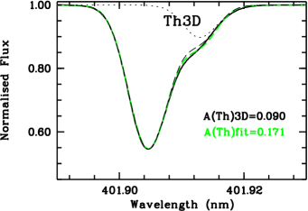
Figure 3: The 3D profile of (Fe i+Ni i) + (Th ii+Co i+V ii) blend in solid black is over-imposed on the $\mathrm{1D}_{\mathrm{LHD}}$ fit (green/grey dashed line). In the plot is also over-imposed (black dashed line) the $\mathrm{1D}_{\mathrm{LHD}}$ with the same abundance as the 3D profile as well as the 3D Th ii+Co i+V ii profile (dotted line).

1 Introduction

The determination of the ages of the older stellar populations in the Galaxy is fundamental for constraining its buildup mechanisms and determining the associated timescales. A variety of dating techniques have been developed, the majority relying on comparing the colour-magnitude-diagram of a stellar population with theoretical isochrones or “fiducial lines” derived from other observed populations (typically globular clusters).

Long lived unstable isotopes of heavy elements such as ²³⁸U and ²³²Th provide an independent method of determining stellar ages. Such elements are generally produced through neutron capture (specifically rapid neutron capture or r-process) and then decay. Their abundance at the present time thus provides a direct estimate of the time passed since they were produced, if their initial abundance can somehow be inferred. This is typically accomplished by measuring some other stable element with a common nucleosynthetic origin together with the radioactive element. Europium (Eu) has long been a typical choice, since its abundance relative to the abundance of thorium can be established from r-process enrichment models (see Francois et al. 1993, Cowan et al. 1999, Ivans et al. 2006). Sneden et al. (2000) used the [Th/Eu] abundance ratio to estimate the age of the old, metal-poor globular cluster M15 to 14 $\pm$3 Gyr. The study was made easier by the fact that M15 shows strong r-process element enhancement ([Eu/Fe]=1.15, [Th/Fe]=0.81, Sneden et al. 2000). Nevertheless, Eu presents some drawbacks as a cosmochronometric reference element: while easily measurable, its atomic mass is substantially different from the one of Th and U. This generally increases uncertainties. In fact, decaying and stable reference elements should both be formed in the same event, which – for heavy n-capture species – can be safely assumed only if the atomic masses of the two elements are similar. This means in practise that, when a stable reference element is used, it should be as massive as possible. Alternatively, where U is measured, the U/Th ratio can be used since the two have very different half-life times. The measurement of U is nevertheless extremely difficult and has been possible only in two metal-poor r-enhanced stars (Cayrel et al., 2001; Hill et al., 2002; Frebel et al., 2007).

Recently, hafnium (Hf, Z=72) has been suggested as a suitable stable reference element. The Hf production rate via the r-process is believed to be strictly tied to the one of thorium, so that their abundance ratio is almost constant regardless of the neutron density in the generating Super Novae (SN) (Kratz et al. 2007). Hafnium is more massive than Eu (stable Eu isotopes are 151 and 153, while A${}_{\rm Hf}\approx 178$) and can be measured from a set of lines in the blue part of the visual spectrum (the most suitable ones being at 391.8 and 409.3 nm) for which accurate transition data have been recently measured (Lawler et al. 2007). On the down-side, Hf is believed to be efficiently produced by s-process (about 55% of the meteoritic Hf content in the solar system is believed to have been produced by the s-process, see Arlandini et al. 1999). As a consequence, it can be effectively employed as a reference only where s-process enrichment can be considered negligible, or if the s-process contribution can be reliably modelled.

Although in principle promising, Hf/Th dating is not free of drawbacks. In the first place an uncertainty of 0.1 dex in [Th/Hf] implies about 4.7 Gyr (see also Ludwig et al., 2008a) uncertainty in the dating. Second, the theoretical prediction of strong ties between Th and Hf production needs to be verified by observations. Third, the applicability of the method to normal (i. e. not r-process enhanced) stars needs some testing: especially Th lines become relatively weak and significant blends can be prejudicial especially in more metal-rich objects.

With the prospect of using hafnium and thorium for dating purposes, we decided to determine the solar hafnium and thorium abundances using hydrodynamical model atmospheres. We anticipate that 3D effects are found to be non-negligible for Th, and mainly due to the convection-induced asymmetry of blending lines.

In the solar spectrum, the measurable lines of Hf are from the singly ionised atom, and are often blended with other photospheric absorption lines. As a consequence, solar photospheric abundance determinations are scarce in the literature. Russell (1929) determined the photospheric hafnium solar abundance to be 0.90. Recently, Lawler et al. (2007) measured Hf lifetimes for several lines, four of which were used to determine a solar photospheric hafnium abundance of $0.88\pm 0.08$. Andersen et al. (1976) considered nine lines of Hf ii (two of which are in common with Lawler et al. 2007) and obtained from a Kitt Peak National Observatory centre-disc spectrum a solar photospheric hafnium abundance of $0.88\pm 0.08$. Values of the meteoritic hafnium abundance cited in literature include: $0.73\pm 0.01$, Anders & Grevesse (1989); $0.75\pm 0.02$ Grevesse & Sauval (1998); and $0.77\pm 0.04$ Lodders (2003).

Thorium is measurable in the Sun from one single line of Th ii at 401.9 nm, which is heavily blended. Solar thorium abundances in literature are very rare. Holweger (1980) derived a Th abundance of 0.16, Anders & Grevesse (1989) report abundances of $0.12\pm 0.06$ from the 401.9 nm line due to an unpublished measurement of Grevesse. Lodders (2003) recommends the meteoritic value A(Th)=$0.09\pm 0.04$ from Grevesse et al. (1996). The meteoritic value is $0.08\pm 0.02$ (Anders & Grevesse, 1989), inferred from the mass-spectroscopically measured ratio of 0.0329 Th atoms to $10^{6}$ Si atoms (Rocholl & Jochum, 1993) in carbonaceous chondrites.

2 Atomic data

We considered the same four Hf ii lines with the same $\log gf$ as Lawler et al. (2007) have been considered (see Table 1). Line parameters for the 401.9 nm Th ii and blending lines in this range are from del Peloso et al. (2005a).

Table 1: Hf ii lines considered in this work.

Wavelength	Transition	Elow	$\log gf$
nm		eV
338.983	a4F–z2P0	0.45	–0.78
356.166	a2D–z4F0	0.00	–0.87
391.809	a4F–z4D0	0.45	–1.14
409.315	a4F–z4P0	0.45	–1.15

3 Models

Our analysis is based on a 3D model atmosphere computed with the $\mathrm{CO}^{5}\mathrm{BOLD}$ code (Freytag et al., 2002; Wedemeyer et al., 2004). In addition to the $\mathrm{CO}^{5}\mathrm{BOLD}$ hydrodynamical simulation we use several 1D models. More details about the applied models can be found in Caffau et al. (2007) and Caffau & Ludwig (2007). As in previous works we call $\left\langle\mathrm{3D}\right\rangle$ the 1D model derived by a horizontal and temporal averaging of the 3D $\mathrm{CO}^{5}\mathrm{BOLD}$ model. The reference 1D model for the computation of the 3D abundance corrections is a hydrostatic 1D model atmosphere computed with the LHD code (see Caffau & Ludwig 2007), hereafter $\mathrm{1D}_{\mathrm{LHD}}$ model. $\mathrm{1D}_{\mathrm{LHD}}$ employs the same micro-physics (opacities, equation-of-state, radiative transfer scheme) as $\mathrm{CO}^{5}\mathrm{BOLD}$, and treats the convective energy transport with mixing-length theory. Here, we set the mixing-length parameter to 1.5. We also use the solar ATLAS 9 model computed by Fiorella Castelli and the Holweger-Müller solar model (Holweger, 1967; Holweger & Müller, 1974). The spectrum synthesis code we employ is Linfor3D for all models.

The 3D $\mathrm{CO}^{5}\mathrm{BOLD}$ solar model covers a time interval of 4300 s, represented by 19 snapshots. This time interval should be compared to a characteristic time scale related to convection. Here we choose the sound crossing time over one pressure scale height at the surface $t_{\mathrm{c}}=H_{\mathrm{P}}/c$ ($H_{\mathrm{P}}$: pressure scale height at $\tau_{\mathrm{ross}}=1$, $c$: sound speed) which amounts to 17.8 s in the solar case. Note, that this time scale is not the time over which the convective pattern changes its appearance significantly. This time scale is significantly longer than $t_{\mathrm{c}}$; e.g., Wedemeyer et al. (2004) obtained from simulations a autocorrelation life time of about 120 s for the convection pattern. However, while $t_{\mathrm{c}}$ does not measure the life time of the convective pattern as such, it provides a reasonably accurate scaling of its life time with atmospheric parameters (e.g., Svensson & Ludwig 2005). Hence, it can be used for the inter-comparison of different 3D models.

The particular solar model used in this paper has a higher wavelength resolution (12 opacity bins) with respect to the model we used to study the solar phosphorus abundance (Caffau et al. 2007). The basic characteristics of the 3D models we consider in this work can be found in Table 2.

Table 2: The $\mathrm{CO}^{5}\mathrm{BOLD}$ models considered in this work.

$T_{\mathrm{eff}}$	$\log g$	[M/H]	$N_{\mathrm{t}}$	time	$t_{\mathrm{c}}$
(K)	(cm s-2)			(s)	(s)
(1)	(2)	(3)	(4)	(5)	(6)
5770	4.44	0.0	19	4300	17.8
4980	4.50	0.0	20	30800	14.8
5060	4.50	–1.0	19	65600	15.1
5430	3.50	0.0	18	144000	151.0
5480	3.50	–1.0	19	106800	149.3
5930	4.00	0.0	18	26400	49.8
5850	4.00	–1.0	18	36600	48.9
5870	4.50	0.0	19	16900	16.0
5920	4.50	–1.0	8	7000	15.7
6230	4.50	0.0	20	35400	16.3
6240	4.50	–1.0	20	25000	16.1
6460	4.50	0.0	20	17400	16.4
6460	4.50	–1.0	20	36200	16.3

Note: Cols.(1), (2), and (3) state the atmospheric parameters of the models; col(4) the number of snapshots $N_{\mathrm{t}}$ considered; col(5) the time interval covered by the selected snapshots; col(6) a characteristic timescale $t_{\mathrm{c}}$ of the evolution of the granular flow.

As in our study of sulphur (see Caffau & Ludwig, 2007) and phosphorus (see Caffau et al., 2007), we define as “3D correction” the difference in the abundance derived from the 3D $\mathrm{CO}^{5}\mathrm{BOLD}$ model and the $\mathrm{1D}_{\mathrm{LHD}}$ model, both synthesised with Linfor3D. We consider also the difference in the abundance derived from the 3D $\mathrm{CO}^{5}\mathrm{BOLD}$ model and from the $\left\langle\mathrm{3D}\right\rangle$ model. Since the 3D $\mathrm{CO}^{5}\mathrm{BOLD}$ and $\left\langle\mathrm{3D}\right\rangle$ models have, by construction, the same mean temperature structure, this allows us to single out the effects due to the horizontal temperature fluctuations.

4 Observational data

The observational data we use consists of two high-resolution, high signal-to-noise ratio spectra of centre disc solar intensity: that of Neckel & Labs (1984) (hereafter referred to as the “Neckel intensity spectrum”) and that of (Delbouille, Roland & Neven, 1973) (hereafter referred to as the “Delbouille intensity spectrum” ). We further use the disc-integrated solar flux spectrum of Neckel & Labs (1984) and the solar flux spectrum of Kurucz (2005), referred to as the “Kurucz flux spectrum”.

5 Data analysis

5.1 Hafnium

The computation of a 3D synthetic spectrum with Linfor3D is rather time consuming and the spectral-synthesis code can handle easily only a few tens of lines. The $\log gf$ values of the lines blending the Hf lines and lying nearby are not well known, and the synthetic spectra do not reproduce the observed solar spectrum well in that region. To fit the line profiles Lawler et al. (2007) changed the $\log gf$ of some lines blending the Hf ii lines, but did not make available the values used. In any case, solar $\log gf$ values derived from 1D and 3D fitting are not guaranteed to be the same. Our computational power is insufficient at the moment to enable us to fit 3D synthetic spectra to an observed spectrum by changing the $\log gf$ values of various lines. Consequently, we could not produce solar $\log gf$ for the blending lines and fit the line profiles with a 3D model grid. Instead of fitting astrophysical solar $\log gf$ of the blending features, we introduced blending components in the process of measuring EW. We thus took advantage of the deblending mode of the IRAF task splot. The corresponding Hf abundance is then derived from the curves of growth computed with Linfor3D for the various lines. The results of Lawler et al. (2007) are used as a check for our measurements. The abundances we obtain from the Holweger-Müller (HM) model are in agreement with their measurement. The results for all spectra and individual lines are presented in Table 3.

Table 3: Solar hafnium abundances from the various observed spectra.

spec	wavelength	EW	A(Hf)					$\sigma$	Ref.	3D-$\mathrm{1D}_{\mathrm{LHD}}$	$\sigma_{\langle{\rm EW}\rangle}$	$\sigma_{\rm A}$
	nm	pm	3D	$\left\langle\mathrm{3D}\right\rangle$	$\mathrm{1D}_{\mathrm{LHD}}$	1DATLAS	1DHM	dex		dex	%	dex
(1)	(2)	(3)	(4)	(5)	(6)	(7)	(8)	(9)	(10)	(11)	(12)	(13)
NI	338.9	0.489	0.911	0.895	0.883	0.900	0.914	0.02		0.029	0.29	0.0013
DI	338.9	0.477	0.899	0.883	0.871	0.886	0.903	0.02	0.91	0.029
NI	356.2	0.845	0.819	0.801	0.781	0.799	0.821	0.01		0.037	0.31	0.0014
DI	356.2	0.851	0.822	0.805	0.785	0.803	0.824	0.02	0.85	0.037
NF	391.8	0.318	0.823	0.827	0.815	0.836	0.848	0.05		0.008	0.26	0.0011
NI	391.8	0.302	0.911	0.899	0.893	0.912	0.925	0.02		0.018	0.27	0.0012
DI	391.8	0.274	0.867	0.854	0.849	0.868	0.881	0.05	0.91	0.018
KF	409.3	0.317	0.814	0.818	0.805	0.826	0.838	0.07		0.010	0.26	0.0011
NF	409.3	0.318	0.816	0.820	0.806	0.828	0.840	0.07		0.010
NI	409.3	0.292	0.886	0.874	0.865	0.884	0.899	0.02		0.020	0.26	0.0011
DI	409.3	0.268	0.847	0.835	0.827	0.846	0.860	0.04	0.86	0.020

Note: Abundances and their uncertainties – if not noted otherwise – are given on the usual logarithmic spectroscopic scale where A(H)=12. Col. (1) is an identification flag, DI means Delbouille and NI Neckel disc-centre spectrum, NF Neckel and KF Kurucz flux spectrum. Col. (4): hafnium abundance, A(Hf), according to the $\mathrm{CO}^{5}\mathrm{BOLD}$ 3D model. Cols. (5)-(8): A(Hf) from 1D models, with $\xi$, micro-turbulence, of 1.0 $\mathrm{km\,s^{-1}}$ . Col. (9): uncertainties related to EW measurement. Col. (10) Lawler et al. (2007). Col. (11): 3D corrections. Col. (12): uncertainty of the theoretical equivalent width due to the limited statistics obtained from the 3D model. Col. (13): uncertainty in abundance due to the model uncertainty in equivalent width.

We determine the following hafnium abundances: $0.870\pm 0.038$ if we consider only the disc-centre intensity spectra, $0.818\pm 0.005$ according to the solar flux spectra, and $0.856\pm 0.040$ if we consider both the intensity and the flux spectra. As final uncertainty we took the line to line RMS scatter over all spectra. Equivalent widths can be measured in both flux spectra only for the 409.3 nm hafnium line, which is nearly free of blends. Only the Neckel flux spectrum can be considered for the Hf line at 391.8 nm, due to the fact that the larger broadening of flux spectra with respect to intensities makes the measurement more difficult, if not impossible. Additionally, NLTE corrections may be different in intensity and flux spectra. For these reasons, and to have a consistent comparison with the results of Lawler et al. (2007), we determine the solar hafnium abundance from the average value stemming from the disc-centre spectra. Our results are in good agreement with the results of Lawler et al. (2007); we obtain A(Hf)=$0.878\pm 0.040$ from the Holweger-Müller model, considering only disc-centre spectra, which is to compare to their value of $0.88\pm 0.02$.

The 3D abundance corrections for Hf are very small. The highest value, 0.037 dex, is the one for the strongest line. As previously mentioned, a 3D correction is the difference in abundance obtained from the 3D model and the $\mathrm{1D}_{\mathrm{LHD}}$ model. If one chooses an ATLAS or the Holweger-Müller model as a 1D reference model, the 3D correction would be even smaller or negative, respectively.

The $\left\langle\mathrm{3D}\right\rangle$ and $\mathrm{1D}_{\mathrm{LHD}}$ solar model temperature structures are similar. The relative contribution to the 3D correction due to different average temperature profiles is small. The 3D correction is larger for stronger lines, quite insensitive to micro-turbulence, of the same order of magnitude for flux and intensity, and slightly higher for intensity.

5.2 Thorium

Singly ionised thorium is the dominant ionisation stage in the solar atmosphere, and thorium is measurable in the Sun only through the 401.9 nm Th ii resonance line. Holweger (1980) detected also the 408.6 nm Th ii line, however in our view this line is too weak and blended to be used for quantitative analysis. The 401.9 nm line happens to fall on the wing of a strong blend of neutral iron and nickel. Additionally, it is blended with a Co i line (about 25% of the EW of the Th ii line) and a weaker V ii line (1/5 of the Co line, 1/9 of the Th line in EW). The Co i and V ii lines are very close in wavelength to the Th ii line, and it is therefore practically impossible to disentangle the blend. Consequently, we do not measure the contribution in EW due to thorium, but instead use the EWs measured by Lawler et al. (1990) to obtain A(Th) (see Table 4, first two lines). However, while Lawler et al. (1990) considered only the contribution of Co i to the blend, we consider also the contribution of V ii. To do so we computed from the $\mathrm{CO}^{5}\mathrm{BOLD}$ solar model the EW of the Co i+V ii blend, using the atomic data from del Peloso et al. (2005a), and subtracted this value from the EW of Lawler et al. (1990). In this manner, we obtained a smaller solar A(Th) (see last two lines of Table 4). The 3D corrections listed in Table 4 are deduced from the EWs alone, and we shall call them in the following “intrinsic” 3D corrections. These are the corrections that would be found if the Th ii line were isolated. Since it is instead found in the middle of a rather complex spectral region, other 3D-related effects arise, which are discussed later.

Table 4: Solar thorium abundances derived from the EWs of Lawler et al. (1990).

spec	EW	A(Th)				$\sigma$	3D-$\left\langle\mathrm{3D}\right\rangle$	3D-$\mathrm{1D}_{\mathrm{LHD}}$	$\sigma_{\rm\langle EW\rangle}$	$\sigma_{\rm A}$
	pm	3D	$\left\langle\mathrm{3D}\right\rangle$	$\mathrm{1D}_{\mathrm{LHD}}$	1DHM				%	dex
(1)	(2)	(3)	(4)	(5)	(6)	(7)	(8)	(9)	(10)	(11)
Int	0.415	0.168	0.164	0.148	0.190	0.022	0.004	0.0207	0.33	0.0015
Flux	0.505	0.135	0.151	0.130	0.172		-0.015	0.0052	0.34	0.0015
Int*	0.355	0.095	0.092	0.075	0.118	0.026	0.003	0.0199
Flux*	0.430	0.060	0.074	0.054	0.096		-0.015	0.0060

Notes: The contribution to the EW of Co and V, according to the 3D simulation, has been been from the EWs in the last two rows (labelled with *). (1) identification flag to distinguish disc-centre to flux spectrum results; (3) thorium abundance, A(Th), according to the $\mathrm{CO}^{5}\mathrm{BOLD}$ 3D model; (4)-(6) A(Th) from 1D models, with $\xi$, micro-turbulence, of 1.0 $\mathrm{km\,s^{-1}}$ ; (7) the uncertainty due to the EW; (8)-(9) 3D corrections; (10) statistical uncertainty of the theoretical EW; (11) corresponding uncertainty in abundance.

Table 5: Solar thorium abundance derived from line profile fitting.

	3D			LHD
	A(Th)	SHIFT	$V_{br}$	A(Th)	SHIFT	$V_{br}$	3D-$\mathrm{1D}_{\mathrm{LHD}}$
	dex	$\mathrm{km\,s^{-1}}$	$\mathrm{km\,s^{-1}}$	dex	$\mathrm{km\,s^{-1}}$	$\mathrm{km\,s^{-1}}$	dex
Int. (Neckel)	0.088	–0.05	1.49	0.160	–0.53	2.77	–0.720
Int. (Delbouille)	0.080	+0.01	1.86	0.168	–0.47	2.99	–0.088
Flux (Neckel)	0.056	–0.39	1.68	0.168	–0.47	4.11	–0.112
Flux (Kurucz)	0.067	–0.38	2.82	0.175	–0.46	4.71	–0.108

Note: (2)-(4) results of the fitting: A(Th), shift, and broadening using a 3D grid; (5)-(7) same for $\mathrm{1D}_{\mathrm{LHD}}$ grid; (8) gives the difference in abundance A(Th)${}_{\rm 3D}-$A(Th)${}_{\rm\mathrm{1D}_{\mathrm{LHD}}}$.

The last two columns of Table 4 provide estimates of the statistical uncertainty of the theoretical EW predicted by the 3D model and the associated uncertainty in the hafnium abundance. The 3D model provides only a statistical realisation of the stellar atmosphere, and is thus subject to limited statistics (see Ludwig et al., 2008b). However, as necessary for a reliable derivation of abundances these uncertainties are insignificant and only added for completeness.

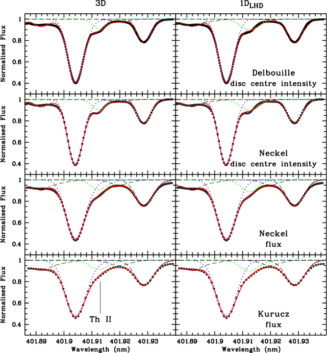
Figure 4: Fits of the synthetic spectra to the observed solar spectra. On the left hand side, the synthetic spectra have been computed from the $\mathrm{CO}^{5}\mathrm{BOLD}$ model, on the right hand side from the corresponding $\mathrm{1D}_{\mathrm{LHD}}$ model. On either side, from top to bottom, the spectra are: the Delbouille disc centre intensity, the Neckel disc centre intensity, the Neckel flux and the Kurucz flux. On each panel the sub-components used to synthesise the feature are shown individually: the light dotted line is the Th ii+Co i+V ii blend, the darker dotted line is the Ni i+Fe i blend, the black dashed lines are, from blue to red, the Mn i+Fe i blend the artificial Fe ii line and the Co i 401.93 nm lines.

Since the Th ii line lies on the red wing of the stronger Fe i+Ni i blend, one can expect that the line asymmetry of the latter contributes in a non-negligible manner to the measured EW. Up to now it has generally been considered that convective line asymmetries have no impact on the derived abundances, which is true, if the line is isolated. Cayrel et al. (2007) have demonstrated that such asymmetries are non-negligible for the derivation of the ⁶Li/⁷Li isotopic ratio. From the purely morphological point of view, the case of the Th ii resonance line is similar to that of the ⁶Li i resonance line: a weak line which falls on the red wing of a stronger line, which is asymmetric due to the effects of convection. In order to investigate this effect one has to consider the full line profile and resort to spectrum synthesis.

To gain some insight into the problem we began by comparing synthetic profiles, which included only the Fe i+Ni i blend and the Th ii+Co i+V ii blend, computed from the $\mathrm{CO}^{5}\mathrm{BOLD}$ and $\mathrm{1D}_{\mathrm{LHD}}$ models. In Fig.2, the $\mathrm{1D}_{\mathrm{LHD}}$ flux profile of the Fe i+Ni i blend has been scaled (since the line strength is different in 1D and 3D) in order to have the same central depth of the 3D profile. The asymmetry of the red wing is obvious. The difference between the 3D and the $\mathrm{1D}_{\mathrm{LHD}}$ profiles is shown in the dotted line of the figure. The 3D thorium profile is also shown as a dashed line and it makes clear that the line asymmetry does indeed contribute to the measured EW. The EW of this difference is 0.134 pm, which translates into a difference in abundance of +0.13 dex for flux. For intensity, $\Delta$(EW) = 0.088 pm implies $\Delta$A(Th)=+0.10 dex in Th abundance.

On a level of slightly higher sophistication with respect to the above naive argument, we fitted the 3D synthetic profile with a grid of $\mathrm{1D}_{\mathrm{LHD}}$ synthetic spectra of differing Th abundance. We scaled the $\mathrm{1D}_{\mathrm{LHD}}$ Fe+Ni blend in order to induce it to have the same central residual intensity as the 3D profile. One of the results of the fitting is shown in Fig. 3: the 3D profile (black solid line) with A(Th)=0.09 when fitted with a $\mathrm{1D}_{\mathrm{LHD}}$ grid (dashed green/grey line) gives a higher abundance A(Th)=0.171. The use of a $\left\langle\mathrm{3D}\right\rangle$ grid leads to an even higher thorium abundance: A(Th)=0.227. In the plot the $\mathrm{1D}_{\mathrm{LHD}}$ flux profile, with the same abundance as the 3D synthetic spectrum, is shown, as well as the 3D thorium profile. For the disc-centre intensity, with the same procedure as used for flux, the fitting of a 3D profile assuming a thorium abundance of 0.09 with a $\mathrm{1D}_{\mathrm{LHD}}$ grid implies A(Th)=0.110, while with a $\left\langle\mathrm{3D}\right\rangle$ grid A(Th)=0.155. The difference of the result of the fit when using $\left\langle\mathrm{3D}\right\rangle$ or $\mathrm{1D}_{\mathrm{LHD}}$ grids is due to the superposition of the effect of the line asymmetry and the “intrinsic” 3D corrections (A(Th)_3D-A(Th)_1D).

The Fe i+Ni i line asymmetry and the 3D corrections act in opposite directions: the line asymmetry produces a higher A(Th) from 1D analysis, while the 3D correction is positive, thus A(Th) from a 1D analysis is smaller. However, the 3D correction in intensity is between 3 and 4 times larger than for flux (see Table 4).

In Fig. 4 we show the results of fitting the whole spectral region both with 3D (left hand side) and $\mathrm{1D}_{\mathrm{LHD}}$ (right hand side) profiles. The synthetic profiles have been built by adding 5 components: a Mn I+Fe I blend centred at 401.89 nm, the Fe i+Ni i blend, the Th ii+Co i+V ii blend, an artificial Fe ii line at 401.9206, initially suggested by Francois et al. (1993) and adopted also by del Peloso et al. (2005a), and the two Co i lines at 401.93. Of these components the Th ii+Co i+V ii blend was computed for three different Th abundances, all the other components were instead computed for a single abundance and were scaled by the fitting procedure in order to best reproduce the observed spectrum.

The results of the fitting are summarised in Table 5. From the table one sees that the total 3D correction, taking into account both line asymmetry and “intrinsic” 3D correction is from –0.07 to –0.09 dex for the intensity spectra and –0.11 dex for the flux spectra. This difference is expected, given that the “intrinsic” 3D correction, as given in Table 4, is about +0.02 dex for intensity and about +0.005 dex for flux.

It is quite interesting to note that in the case of Th the line asymmetry implies a total 3D effect which is not only much larger, but also in a different direction, from what would have been implied by the “intrinsic” 3D correction. To our knowledge this is the second time such an effect has been highlighted. These “total” 3D corrections are only slightly larger than what was estimated above from the fit of the 3D Fe i+Ni i blend plus Th ii+Co i+V ii blend, with $\mathrm{1D}_{\mathrm{LHD}}$ profiles. This suggests that the use of the simpler procedure is still capable of providing the correct order of magnitude for the “total” 3D correction. Finally we point out that, as can be seen from the left hand side of Fig.4, it is obvious that the $\mathrm{1D}_{\mathrm{LHD}}$ profiles are unable to provide the correct shape for the Th feature. The shape is reproduced in a much more satisfactory way by the 3D profiles.

We conclude this section by investigating the iron line at 401.9 nm, which is the stronger component of the Fe i+Ni i blend. The 3D synthetic line shows a strong asymmetry; the difference 3D-1D is very pronounced on the red wing if we make an appropriate shift and broadening to the 1D profile so as to over-impose the blue wings of the 3D and 1D synthetic spectra. While the flux of the 3D synthetic spectrum is shifted to the blue by 0.1 $\mathrm{km\,s^{-1}}$ , the intensity spectra, corresponding to different inclination angles, show a shift ranging from -0.5 $\mathrm{km\,s^{-1}}$  to +0.15 $\mathrm{km\,s^{-1}}$ .

6 The 3D effects for other models.

6.1 Hafnium

Beyond the solar model as such we investigated the hydrodynamical effects on some other 3D models of dwarf and sub-giant stars (see Table 2). We restricted our investigation to solar or –1.0 metallicity, because for lower metallicity these hafnium lines are no longer measurable in dwarfs. Even the detection at –1.0 metallicity is only possible for the strongest of the hafnium lines, but the two metallicities can be used for interpolation to intermediate metallicity. We find that 3D and 1D abundances are generally very similar, making the 3D corrections insignificant for all models and all lines we consider.

Hf ii is the dominant species of hafnium in the photosphere of these models. Both the 5900 K models predict that at least 98% of the Hf is ionised. The hotter models foresee an even lower fraction of Hf i. The coolest models at 5000 K predict that at least 75% of the Hf is ionised. The results are similar when considering the $\left\langle\mathrm{3D}\right\rangle$ or the $\mathrm{1D}_{\mathrm{LHD}}$ temperature profile for the atmosphere.

If we compare the horizontal average temperature profile of the 3D model to the $\mathrm{1D}_{\mathrm{LHD}}$ model we can see that they are very similar. There is no pronounced cooling of the 3D atmospheres relative to $\mathrm{1D}_{\mathrm{LHD}}$ in radiative equilibrium for the same atmospheric parameters which is known to be prominent in more metal-poor models.

Table 6: Non-solar $\mathrm{CO}^{5}\mathrm{BOLD}$ models considered in this work.

Wavelength	EW	A(Hf)			3D-$\left\langle\mathrm{3D}\right\rangle$	3D-$\mathrm{1D}_{\mathrm{LHD}}$	$\sigma_{\rm\langle EW\rangle}$	$\sigma_{\rm A}$
nm	pm	3D	$\left\langle\mathrm{3D}\right\rangle$	$\mathrm{1D}_{\mathrm{LHD}}$			%	dex
(1)	(2)	(3)	(4)	(5)	(6)	(7)	(8)	(9)
5060/4.5/0.0
339.0	0.718	0.870	0.842	0.829	0.028	0.041	0.05	0.0002
356.2	1.550	0.872	0.809	0.796	0.062	0.076	0.09	0.0003
391.8	0.405	0.870	0.854	0.841	0.016	0.029	0.07	0.0003
409.3	0.410	0.870	0.855	0.841	0.016	0.029	0.07	0.0003
5060/4.5/-1.0
339.0	0.151	0.870	0.866	0.852	0.004	0.018	0.11	0.0005
356.2	0.395	0.870	0.864	0.852	0.007	0.018	0.12	0.0005
391.8	0.080	0.870	0.870	0.855	0.001	0.015	0.11	0.0005
409.3	0.081	0.868	0.867	0.853	0.001	0.015	0.11	0.0005
5870/4.5/0.0
339.0	0.551	0.870	0.862	0.858	0.008	0.011	0.20	0.0008
356.2	1.150	0.870	0.857	0.849	0.012	0.020	0.22	0.0010
391.8	0.330	0.871	0.867	0.869	0.004	0.002	0.18	0.0008
409.3	0.336	0.870	0.867	0.867	0.003	0.003	0.18	0.0008
5920/4.5/–1.0
3390.	0.095	0.871	0.872	0.868	-0.001	0.003	0.57	0.0025
3562.	0.230	0.870	0.880	0.881	-0.010	-0.011	0.67	0.0029
3918.	0.053	0.869	0.872	0.873	-0.003	-0.004	0.55	0.0024
4093.	0.054	0.866	0.869	0.870	-0.003	-0.004	0.56	0.0026
6230/4.5/0.0
339.0	0.444	0.870	0.865	0.859	0.005	0.012	0.22	0.0009
356.2	0.916	0.870	0.865	0.855	0.004	0.015	0.25	0.0011
391.8	0.275	0.870	0.866	0.870	0.004	-0.001	0.19	0.0008
409.3	0.281	0.870	0.866	0.869	0.003	0.001	0.20	0.0009
6240/4.5/–1.0
339.0	0.073	0.869	0.876	0.870	-0.007	-0.001	0.19	0.0008
356.2	0.173	0.871	0.889	0.889	-0.018	-0.018	0.20	0.0009
391.8	0.042	0.866	0.874	0.876	-0.008	-0.010	0.17	0.0007
409.3	0.044	0.875	0.884	0.885	-0.009	-0.010	0.17	0.0007
6460/4.5/0.0
339.0	0.374	0.871	0.869	0.864	0.002	0.006	0.23	0.0010
356.2	0.764	0.870	0.871	0.863	0.000	0.007	0.26	0.0011
391.8	0.239	0.869	0.868	0.877	0.002	-0.008	0.20	0.0009
409.3	0.245	0.871	0.869	0.877	0.002	-0.006	0.20	0.0009
6460/4.5/–1.0
339.0	0.059	0.867	0.883	0.875	-0.016	-0.007	0.25	0.0011
356.2	0.137	0.868	0.897	0.897	-0.029	-0.029	0.27	0.0012
391.8	0.035	0.865	0.881	0.882	-0.016	-0.017	0.21	0.0009
409.3	0.036	0.866	0.883	0.883	-0.016	-0.017	0.21	0.0009
5500/3.5/0.0
339.0	1.500	0.868	0.855	0.850	0.014	0.019	0.23	0.0010
356.2	2.780	0.871	0.845	0.830	0.026	0.041	0.29	0.0012
391.8	0.987	0.870	0.865	0.867	0.005	0.003	0.21	0.0009
409.3	1.000	0.868	0.864	0.863	0.004	0.005	0.22	0.0009
5500/3.5/–1.0
339.0	3.160	0.870	0.870	0.863	0.001	0.007	0.29	0.0013
356.2	0.758	0.870	0.874	0.862	-0.003	0.008	0.34	0.0015
391.8	0.182	0.871	0.874	0.872	-0.003	-0.001	0.28	0.0012
409.3	0.186	0.871	0.875	0.870	-0.004	0.001	0.29	0.0013

Note: The atmospheric parameters are given as $T_{\mathrm{eff}}$/$\log g$/[M/H]. cols. (3)-(5) are the A(Hf), according to $\mathrm{CO}^{5}\mathrm{BOLD}$ 3D, $\left\langle\mathrm{3D}\right\rangle$  and $\mathrm{1D}_{\mathrm{LHD}}$ model; cols. (6)-(7) are 3D corrections, 3D-$\left\langle\mathrm{3D}\right\rangle$ and 3D-$\mathrm{1D}_{\mathrm{LHD}}$ respectively; col. (8) statistical uncertainty of the theoretical EW; col. (9) corresponding uncertainty in abundance.

6.2 Thorium

As for hafnium and as in the solar case, the “intrinsic” 3D corrections are small for the other models. The hydrodynamical effects are instead due to the line asymmetry, like in the Sun. When we fit, as we do for the Sun, a 3D flux profile, with meteoritic or scaled meteoritic A(Th) for the metal-poor models, with a $\mathrm{1D}_{\mathrm{LHD}}$ grid we obtain for A(Th) a value higher by 0.08-0.12 dex considering the models: 5500 K/3.50/0.0, 5500 K/3.50/–1.0 5900 K/4.00/0.0, 5900 K/4.00/–1.0, 5900 K/4.50/0.0, and 5900 K/4.50/–1.0 (see Table 2). One has to keep in mind that such differences translate into systematic age differences of almost 5 Gyr in the context of nucleocosmochronology.

7 Conclusions

Our determination of the photospheric hafnium abundance, A(Hf)=$0.87\pm 0.04$, derived from a 3D hydrodynamical $\mathrm{CO}^{5}\mathrm{BOLD}$ solar model, is very close to the abundance determination of Lawler et al. (2007) obtained using the Holweger-Müller solar model. The EWs of the hafnium lines are not very sensitive to the hydrodynamical effects. A difference of the same amount of the 3D correction can be found if we compare the A(Hf) obtained using two different 1D models, such as ATLAS and Holweger-Müller model or $\mathrm{1D}_{\mathrm{LHD}}$ and the Holweger-Müller model. These difference are related to different opacities and physics used to compute the models. Synthetic profiles of hafnium lines computed from 3D models show a pronounced asymmetry, but this effect is not relevant for abundance determination as long as only the EW is considered.

For thorium, as for hafnium, 3D effects on the EWs are less than or comparable to the uncertainties related to the EW measurement, so that they are negligible when determining A(Th). However, for the solar photospheric thorium determination the asymmetry of the strong Fe i+Ni i line blending the 401.9 nm Th ii weak line implies a non-negligible effect on the derived Th abundance and is in fact the dominant source of the “total” 3D effect. The asymmetry is a hydrodynamical effect, and we find a difference in the A(Th) determination of about –0.1 dex when considering this asymmetry. Our results for the Sun and for other 3D dwarfs and sub-giants models imply that Th cannot be reliably measured without making use of hydrodynamical simulation if the Th line is weak and blended. A reappraisal of existing Th measurements in the light of hydrodynamical simulations is warranted for dwarfs and sub-giants.