Public transport networks: empirical analysis and modeling

Abstract

We use complex network concepts to analyze statistical properties of urban public transport networks (PTN). To this end, we present a comprehensive survey of the statistical properties of PTNs based on the data of fourteen cities of so far unexplored network size. Especially helpful in our analysis are different network representations. Within a comprehensive approach we calculate PTN characteristics in all of these representations and perform a comparative analysis. The standard network characteristics obtained in this way often correspond to features that are of practical importance to a passenger using public traffic in a given city. Specific features are addressed that are unique to PTNs and networks with similar transport functions (such as networks of neurons, cables, pipes, vessels embedded in 2D or 3D space). Based on the empirical survey, we propose a model that albeit being simple enough is capable of reproducing many of the identified PTN properties. A central ingredient of this model is a growth dynamics in terms of routes represented by self-avoiding walks.

I Introduction

The general interest in networks of man-made and natural systems has lead to a careful analysis of various network instances using empirical, simulational, and theoretical tools. The emergence of this field is sometimes referred to as the birth of network science Barabasi02 ; Dorogovtsev02 ; Newman03a ; Dorogovtsev03 ; Holovatch06 . In this paper, we use complex network concepts to analyze the statistical properties of public transport networks (PTN) of large cities. These constitute an example of transportation networks Newman03a and share general features of these systems: evolutionary dynamics, optimization, embedding in two dimensional (2D) space. Other examples of transportation networks are given by the airport Amaral00 ; Guimera04 ; Guimera05 ; Barrat04 ; Chi03 ; He04 ; Li04 ; Li06 , railway Sen03 , or power grid networks Amaral00 ; Crucitti04 ; Albert04 .

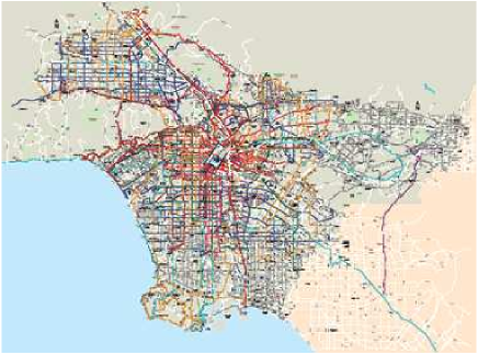
Figure 1: One of the networks we analyze in this study. The Los Angeles PTN consists of $R=1881$ routes and $N=44629$ stations, some of them are shown in this map (color online).

While the evolution of a PTN of a given city is closely related to the city growth itself and therefore is influenced by numerous factors of geographical, historical, and social origin, there is ample evidence that PTNs of different cities share common statistical properties that arise due to their functional purposes Marchiori00 ; Latora01 ; Latora02 ; Seaton04 ; Ferber05 ; Sienkiewicz05 ; Angeloudis06 ; Zhang06 ; Ferber07a ; Chang07 ; Xu07 ; Ferber07b ; Ferber07c . Some of these properties have been analyzed in former studies, however, the objective of the present study is to present a comprehensive survey of characteristics of PTNs and to provide a comparative analysis. Based on this empirical survey we are in the position to propose a growth model that captures many of the main (statistical) features of PTNs.

A further distinct feature of our study is that the PTNs we will consider are networks of all means of public transport of a city (buses, trams, subway, etc.) regardless of the specific means of transport. A number of studies have analyzed specific sub-networks of PTNs Marchiori00 ; Latora01 ; Latora02 ; Seaton04 ; Angeloudis06 ; Zhang06 ; Xu07 . Examples are the Boston Marchiori00 ; Latora01 ; Latora02 ; Seaton04 and Vienna Seaton04 subway networks and the bus networks of several cities in China Zhang06 ; Xu07 . However, each particular traffic system (e.g. the network of buses or trams, or the subway network) is not a closed system: it is a subgraph of a wider transportation system of a city, or as we call it here, of a PTN. Therefore to understand and describe the properties of public transport in a city as a whole, one should analyze the complete network, without restriction to specific parts. Indeed, for the case of Boston it has been shown that changing from the subway system to the network “subway + bus” the network properties change drastically Latora01 ; Latora02 .

Urban public transport networks of general type have so far been analyzed mainly in two previous studies Ferber05 ; Sienkiewicz05 . In the first one, Ref. Ferber05 , the PTNs of Berlin, Düsseldorf, and Paris were examined, whereas the subject of Ref. Sienkiewicz05 were public transport systems of 22 Polish cities. Ref. Ferber05 concentrated on the scale-free properties. For the cities considered, the node degree distribution was shown to follow a power law. Moreover power laws were found for a number of other specific features describing the traffic load on the PTN. However, the statistics in this study was too small for definite conclusions. In Ref. Sienkiewicz05 it was found that the node degree distribution may follow a power law or be described by an exponential function, depending on the assumed network representation. Besides, a number of other network characteristics (clustering, betweenness, assortativity) were extensively analyzed.

In the present paper, we analyze PTNs of a number of major cities of the world (see table 1) database1 ; database2 . Our choice for this data base was motivated by the requirement to collect network samples from cities of different geographical, cultural, and economical background. Our current analysis extends former studies Ferber05 ; Sienkiewicz05 by considering cities with larger public transport systems (the typical number of stops in the systems considered in Ref. Sienkiewicz05 was several hundreds) as well as by systematically analyzing different representations. The idea of different network representations naturally arises in the network science Barabasi02 ; Dorogovtsev02 ; Newman03a ; Dorogovtsev03 ; Holovatch06 . For the PTN the primary network topology is given by the set of routes each servicing an ordered series of given stations (see Fig. 1 as an example). For the transportation networks studied so far mainly two different neighborhood relations were used. In the first one, two stations are defined as neighbors only if one station is the successor of the other in the series serviced by this route Latora01 ; Latora02 . In the second one, two stations are neighbors whenever they are serviced by a common route Sen03 . We will exploit both representations in our study. Moreover, we introduce further natural representations (described in detail in Section II) which make the description of the PTNs of table 1 comprehensive. In particular, this includes a bipartite graph representation of a transportation network that reflects its intrinsic features Seaton04 ; Zhang06 ; Chang07 .

City	$A$	$P$	$N$	$R$	$S$	Type
Berlin	892	3.7	2992	211	29.4	BSTU
Dallas	887	1.2	5366	117	59.9	B
Düsseldorf	217	0.6	1494	124	28.5	BST
Hamburg	755	1.8	8084	708	25.5	BFSTU
Hong Kong	1052	7.0	2024	321	39.6	B
Istanbul	1538	11.1	4043	414	31.7	BST
London	1577	8.3	10937	922	34.2	BST
Los Angeles	1214	3.8	44629	1881	52.9	B
Moscow	1081	10.5	3569	679	22.2	BEST
Paris	2732	10.0	3728	251	38.2	BS
Rome	5352	4.0	3961	681	26.8	BT
Saõ Paolo	1523	10.9	7215	997	58.3	B
Sydney	1687	3.6	1978	596	16.3	B
Taipei	2457	6.8	5311	389	70.5	B

Table 1: Cities analyzed in this study. $A$: urban area (km²); $P$: population (million inhabitants); $N$: number of PTN stations; $R$: number of PTN routes; $S$: mean route length. Type of transport which is taken into account in the PTN database: Bus, Electric trolleybus, Ferry, Subway, Tram, Urban train.

There is another reason to seek scale-free properties of PTNs considering a larger data base of more cities with larger public transport communications involved. A currently well accepted mechanism to explain the abundant occurrence of power laws is that of preferential attachment or “rich gets richer” Simon55 ; Price76 ; prefattach . As far as PTNs obviously are evolving networks, their evolution may be expected to follow a similar underlying mechanisms. However, scale-free networks have also been shown to arise when minimizing both the effort for communication and the cost for maintaining connections optimization ; Gastner04 . Moreover, this kind of an optimization was shown to lead to small world properties Mathias01 and to explain the appearance of power laws in a general context zipfoptimal . Therefore, scale-free behavior of PTNs may also be related to obvious objectives to optimize their operation.

This paper is organized as follows. In the next section (II) we define different representations in which the PTN will be analyzed, sections III-V explore the network properties in these representations. We separately analyze local characteristics, such as node degrees and clustering coefficients (section III), and global characteristics, such as path length distributions and centralities (section IV). Special attention is paid to characteristics that are unique to PTNs and networks with similar construction principles. An example is given by the analysis of sequences of routes which go in parallel along a given sequence of stations, a feature we call ’harness’ effect. A description of correlations between the properties of neighboring nodes in terms of generalized assortativities is performed in section V. Our findings for the statistics of real-word PTNs are supported by simulations of an evolutionary model of PTNs as displayed in section VI. Conclusions and an outlook are given in section VII. Some of our results have been preliminary announced in Ref. Ferber07a .

II PT network topology

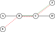
a	b
c	d
e	f

Figure 2: a: a piece of public transport map. Stations A-F are serviced by the tram lines No 1 (solid line), No 2 (dashed line), No 3 (dotted line). Taking all the lines to be indistinguishable, we call such representation $\mathds{L}^{\prime}$-space. b: $\mathds{L}$-space. c: $\mathds{P}^{\prime}$-space. All stations that belong to the same route are connected. d: $\mathds{P}$-space. e: $\mathds{C}^{\prime}$-space. Each route is represented by a node, each link corresponds to a common station shared by the route nodes it connects. f: $\mathds{C}$-space.

Although everyone has an intuitive idea about what a PTN is, it appears that there are numerous ways to define its topology. Let us describe some of them, defining different ’spaces’ in which public transport networks will be analyzed. A straightforward representation of a PT map in the form of a graph represents every station by a node while any two nodes that are successively serviced by at least one route are linked by an edge as shown in Fig. 2a. Let us note, that the full information about the network of $N$ stations and $R$ routes is given by the set of ordered lists each corresponding to one route or to one of the two directions of a given route. These simply list all stations serviced by that route in the order of service between two terminal stations or in the course of a round trip. Note that multiple entries of a given station in such a list are possible and do occur. Let us first introduce a simple graph to represent this situation. In the following we will refer to this graph as a $\mathds{L}$-space Sienkiewicz05 . This graph represents each station by a node, a link between nodes indicates that there is at least one route that services the corresponding station consecutively. No multiple links are allowed (see Fig. 2b). The neighbors of a given node in $\mathds{L}$-space represent all stations that are within reach of a single station trip. For analyzing PTNs, the $\mathds{L}$-space representation has been used in Refs. Latora01 ; Ferber05 ; Sienkiewicz05 ; Angeloudis06 ; Xu07 . Extending the notion of $\mathds{L}$-space one may either introduce multiple links between nodes depending on the number of services between them or associate a corresponding weight to a single link. We will refer to such a representation as $\mathds{L}^{\prime}$-space (c.f. Fig. 2a).

A particularly useful concept for the description of connectivity in transport networks which we refer to as $\mathds{P}$-space Sienkiewicz05 was introduced in ref. Sen03 and used in PTN analysis in Refs. Seaton04 ; Sienkiewicz05 ; Xu07 . In this representation the network is a graph where stations are represented by nodes that are linked if they are serviced by at least one common route. In $\mathds{P}$-space representation the neighborhood of a given node represents all stations that can be reached without changing means of transport. The $\mathds{P}$-space concept may be extended to include multiple or weighted links. Such a representation we refer to as $\mathds{P}^{\prime}$-space (c.f. Figs. 2c and 2d, correspondingly).

A somewhat different concept is that of a bipartite space which is useful in the analysis of cooperation networks Newman03a ; Guillaume06 . In this representation which we call $\mathds{B}$-space both routes and stations are represented by nodes Ferber07a ; Zhang06 ; Chang07 . Each route node is linked to all station nodes that it services. No direct links between nodes of same type occur (see Fig. 3). Obviously, in $\mathds{B}$-space the neighbors of a given route node are all stations that it services while the neighbors of a given station node are all routes that service it.

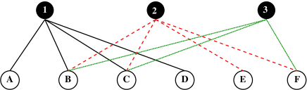
Figure 3: A bipartite graph of tram lines (filled circles) and stations (circles) which corresponds to the public transport map of Fig. 2a. For the sake of illustration, lines corresponding to different tram routes are shown in a differing way. However, neither line type nor the order of the stations matter in this graph. Note that Figs. 2c - 2f are the one-mode projections of this bipartite graph.

We note that the one mode projections of the bipartite graph of $\mathds{B}$-space to the set of station nodes results in $\mathds{P}$-space or in $\mathds{P}^{\prime}$-space space if we retain multiple links. The complementary projection to route nodes leads to a graph which we call $\mathds{C}$-space ($\mathds{C}^{\prime}$-space if multiple links are retained). In this space all nodes represent routes and the neighbors of any route node are those routes with which it shares a common station, see Figs. 2e, 2f.

City	$\langle k_{\mathds{L}}\rangle$	$z_{\mathds{L}}$	$\ell_{\mathds{L}}^{\rm max}$	$\langle\ell_{\mathds{L}}\rangle$	$\langle{\cal C_{\mathds{L}}}^{b}\rangle$	$c_{\mathds{L}}$	$\langle k_{\mathds{P}}\rangle$	$z_{\mathds{P}}$	$\ell_{\mathds{P}}^{\rm max}$	$\langle\ell_{\mathds{P}}\rangle$	$\langle{\cal C_{\mathds{P}}}^{b}\rangle$	$c_{\mathds{P}}$	$\langle k_{\mathds{C}}\rangle$	$z_{\mathds{C}}$	$\ell_{\mathds{C}}^{\rm max}$	$\langle\ell_{\mathds{C}}\rangle$	$\langle{\cal C_{\mathds{C}}}^{b}\rangle$	$c_{\mathds{C}}$
Berlin	2.58	1.96	68	18.5	2.6$\cdot 10^{4}$	52.8	56.61	11.47	5	2.9	2.9$\cdot 10^{3}$	41.9	27.56	4.43	5	2.2	1.2$\cdot 10^{2}$	4.75
Dallas	2.18	1.28	156	52.0	1.4$\cdot 10^{5}$	55.0	100.58	11.23	8	3.2	5.9$\cdot 10^{3}$	48.6	11.09	3.45	7	2.7	9.2$\cdot 10^{1}$	5.34
Düsseldorf	2.57	1.96	48	12.5	8.6$\cdot 10^{3}$	24.4	59.01	10.56	5	2.6	1.2$\cdot 10^{3}$	19.7	32.18	2.47	4	1.8	4.9$\cdot 10^{1}$	2.23
Hamburg	2.65	1.85	156	39.7	1.4$\cdot 10^{5}$	254.7	50.38	7.96	11	4.7	1.4$\cdot 10^{4}$	132.2	17.51	4.49	10	4.0	9.9$\cdot 10^{2}$	28.3
Hong Kong	3.59	3.24	60	11.0	1.0$\cdot 10^{4}$	60.3	125.67	10.20	4	2.2	1.3$\cdot 10^{3}$	11.7	98.98	2.12	3	1.7	1.2$\cdot 10^{2}$	2.14
Istanbul	2.30	1.54	131	29.7	5.7$\cdot 10^{4}$	41.0	76.88	10.59	6	3.1	4.2$\cdot 10^{3}$	41.5	52.81	3.86	5	2.3	2.6$\cdot 10^{2}$	5.00
London	2.60	1.87	107	26.5	1.4$\cdot 10^{5}$	320.6	90.60	16.97	6	3.3	1.2$\cdot 10^{4}$	90.0	49.91	6.80	6	2.6	7.4$\cdot 10^{2}$	11.1
Los Angeles	2.37	1.59	210	37.1	7.9$\cdot 10^{5}$	645.3	97.99	17.21	11	4.4	7.4$\cdot 10^{4}$	399.6	40.11	8.42	10	3.6	2.3$\cdot 10^{3}$	22.1
Moscow	3.32	6.25	27	7.0	1.1$\cdot 10^{4}$	127.4	65.47	26.48	5	2.5	2.7$\cdot 10^{3}$	38.0	109.37	4.57	4	1.9	3.2$\cdot 10^{2}$	3.59
Paris	3.73	5.32	28	6.4	1.0$\cdot 10^{4}$	78.5	50.92	24.06	5	2.7	3.1$\cdot 10^{3}$	59.6	39.95	4.67	4	1.9	1.1$\cdot 10^{2}$	2.72
Rome	2.95	2.02	87	26.4	5.0$\cdot 10^{4}$	163.4	69.05	11.34	6	3.1	4.2$\cdot 10^{3}$	41.4	59.40	4.86	5	2.5	5.1$\cdot 10^{2}$	7.04
Saõ Paolo	3.21	4.17	33	10.3	3.4$\cdot 10^{4}$	268.0	137.46	19.61	5	2.7	6.0$\cdot 10^{3}$	38.2	151.72	4.25	4	2.0	5.2$\cdot 10^{2}$	4.27
Sydney	3.33	2.54	34	12.3	7.3$\cdot 10^{3}$	82.9	42.88	7.79	7	3.0	1.3$\cdot 10^{3}$	33.6	65.02	2.92	6	2.4	3.5$\cdot 10^{2}$	6.30
Taipei	3.12	2.42	74	20.9	5.3$\cdot 10^{4}$	186.2	236.65	12.96	6	2.4	3.6$\cdot 10^{3}$	15.4	93.33	2.95	5	1.8	1.6$\cdot 10^{2}$	2.44

Table 2: PTN characteristics in different spaces (subscripts refer to $\mathds{L}$, $\mathds{P}$, and $\mathds{C}$-spaces, correspondingly). $k$: node degree (nearest neighbors number $z^{(1)}$); $z=\langle z^{(2)}\rangle/\langle z^{(1)}\rangle$ ($z^{(2)}$ being the next nearest neighbors number); $\ell^{\rm max}$, $\langle\ell\rangle$: maximal and mean shortest path length (10); ${\cal C}^{b}$: betweenness centrality (23); $c$: relation of the mean clustering coefficient to that of the classical random graph of equal size (8). Averaging has been performed with respect to corresponding network, only the mean shortest path $\langle\ell\rangle$ is calculated with respect to the largest connected component.

Below, we will study different features of the PT networks as they appear when represented in the above defined spaces. It is worthwhile to mention here, that standard network characteristics being represented in different spaces turn out to be natural characteristics one is interested in when judging about the public transport of a given city. To give an example, the average length of a shortest path $\langle\ell\rangle$ in $\mathds{L}$-space, $\langle\ell_{\mathds{L}}\rangle$ gives the number of stops one has to pass on average to travel between any two stations. When represented in $\mathds{P}$ space, $\langle\ell_{\mathds{P}}\rangle$ tells about how many changes one has to do to travel between any two stations. And, finally, $\langle\ell_{\mathds{C}}\rangle$ brings about the number of changes one has to do to pass between any two routes. Another example is given by the node degree $k$: $k_{\mathds{L}^{\prime}}$ tells to how many directions a passenger can travel at a given station; $k_{\mathds{L}}$ is the number of stops in the direct neighborhood; $k_{\mathds{P}}$ is the number of other stations reachable without changing a line; whereas $k_{\mathds{C}}$ tells how many routes are directly accessible from the given one.

Table 2 lists some of the PTN characteristics we obtained for the cities under consideration using publicly available data from the web pages of local transport organizations database1 ; database2 . A detailed analysis and discussion is given in the following sections III - V.

III Local network characteristics

Let us first examine local properties of the PTNs under discussion. Instead of looking for characteristics of individual nodes we will be interested in their mean values and statistical distributions. This approach allows us to derive conclusions that are significant for the global behavior of the given network. The simplest but highly important properties are those concerning the node degrees of a network and in particular their distribution. Early attempts to model complex networks were performed by mathematicians using the concept of random networks Erdos ; Bollobas85 in which correlations are absent. A wealth of insight was gained by elaborating the theory on rigorous grounds developing many concepts which remain among the core of network analysis. A random graph is given by a set of $N$ nodes and $M$ links. The nodes to which the two ends of each link are connected are chosen with constant probability $2M/N$. In case that multiple links are excluded the average number of neighbors $z_{1}$ is equal to the average node degree $k$ which is:

$$\langle z_{1}\rangle=\langle k\rangle=2M/N.$$ (1)

For the node degree $k$ and its moments $k^{m}$ the average (1) can also be considered as an average with respect to the node degree distribution $p(k)$:

$$\langle k^{m}\rangle=\sum_{k=1}^{\rm k^{\rm max}}p(k)k^{m},$$ (2)

with the obvious notation $k^{\rm max}$ for the maximal node degree. In (2), $\langle\dots\rangle$ stands for an ensemble average over different network configurations. In the following analyzing empirical data we will often use the same notation for an average over a large network instance. For classical random graphs of finite size the node degree distribution $p(k)$ is binomial, in the infinite case it becomes a Poisson distribution.

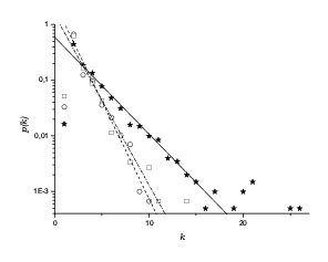
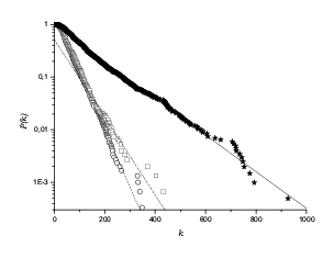
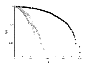
a                                                     b                                                     c

Figure 4: a: Node degree distributions of PTN of several cities in $\mathds{L}$-space. b: Cumulative node degree distribution in $\mathds{P}$-space. c: Cumulative node degree distribution in $\mathds{C}$-space. Berlin (circles, $\hat{k}_{\mathds{L}}=1.24$, $\hat{k}_{\mathds{P}}=39.7$), Düsseldorf (squares, $\hat{k}_{\mathds{L}}=1.43$, $\hat{k}_{\mathds{P}}=58.8$), Hong Kong (stars, $\hat{k}_{\mathds{L}}=2.50$, $\hat{k}_{\mathds{P}}=125.1$).

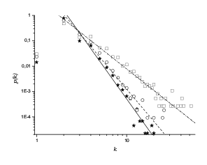
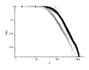
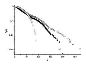
a                                                     b                                                     c

Figure 5: a: Node degree distributions of PTN of several cities in $\mathds{L}$-space. b: Cumulative node degree distributions in $\mathds{P}$-space. c: Cumulative node degree distribution in $\mathds{C}$-space. London (circles, $\gamma_{\mathds{L}}=4.48$, $\gamma_{\mathds{P}}=4.39$), Los Angeles (stars, $\gamma_{\mathds{L}}=4.85$, $\gamma_{\mathds{P}}=3.92$), Paris (squares, $\gamma_{\mathds{L}}=2.62$, $\gamma_{\mathds{P}}=3.70$).

In Figs. 4, 5 we show node degree distributions for PTNs of several cities in $\mathds{L}$, $\mathds{P}$, and $\mathds{C}$-spaces. Note that to get smoother curves we plot in the case of $\mathds{P}$ and $\mathds{C}$-spaces the cumulative distributions defined as:

$$P(k)=\sum_{q=k}^{k^{\rm max}}p(q).$$ (3)

In Fig. 4 the data is shown in a log-linear plot together with fits (for $\mathds{L}$ and $\mathds{P}$-spaces) to an exponential decay:

$$p(k)\sim\exp(-k/\hat{k}),$$ (4)

where $\hat{k}$ is of the order of the mean node degree. Within the accuracy of the data both $\mathds{L}$ and $\mathds{P}$-space distributions for the cities analyzed in Fig. 4 are nicely fitted by an exponential decay. As far as the $\mathds{L}$-space data is concerned, we find evidence for an exponential decay for about half of the cities analyzed, while the other part rather demonstrate a power law decay of the form:

$$p(k)\sim 1/k^{\gamma}.$$ (5)

Figs. 5a, 5b show the corresponding plots for three other cities on a log-log scale. Numerical values of the fit parameters $\hat{k}$ and $\gamma$ (4), (5) for different cities are given in Table 3. There, bracketed values indicate a less reliable fit. Note that for ${\mathds{L}}$-space the fit was done directly for the node degree distribution $p(k)$, whereas due to an essential scattering of data in ${\mathds{P}}$-space the cumulative distribution (3) was fitted and the corresponding values for the fit parameters $\gamma_{\mathds{P}}$, $\hat{k}_{\mathds{P}}$ were extracted from those for the cumulative distributions.

City	$\gamma_{\mathds{L}}$	$\hat{k}_{\mathds{L}}$	$\gamma_{\mathds{P}}$	$\hat{k}_{\mathds{P}}$
Berlin	(4.30)	1.24	(5.85)	39.7
Dallas	5.49	(0.78)	(4.67)	76.9
Dus̈seldorf	(3.76)	1.43	(4.62)	58.8
Hamburg	(4.74)	1.46	(4.38)	60.7
Hong Kong	(2.99)	2.50	(4.40)	125.1
Istanbul	4.04	(1.13)	(2.70)	71.4
London	4.48	(1.44)	4.39	(143.3)
Los Angeles	4.85	(1.52)	3.92	(201.0)
Moscow	(3.22)	2.15	(2.91)	50.0
Paris	2.62	(3.30)	3.70	(100.0)
Rome	3.95	(1.71)	(5.02)	54.8
Saõ Paolo	2.72	(4.20)	(4.06)	225.0
Sydney	4.03	(1.88)	(5.66)	38.7
Taipei	(3.74)	1.75	(5.16)	201.0

Table 3: Parameters of the PTN node degree distributions fit to an exponential (4) and power law (5) behavior. Bracketed values indicate less reliable fits. Subscripts refer to $\mathds{L}$ and $\mathds{P}$-spaces database2 .

While the node degree distribution of almost half of the cities in the $\mathds{L}$-space representation display a power law decay (5), this is not the case for the $\mathds{P}$-space. So far, the analysis of PTNs of smaller cities never showed any power-law behavior in $\mathds{P}$-space Sienkiewicz05 ; Xu07 . The data for the three cities shown in Fig. 5b gives first evidence of power law behavior of $P(k)$ in the $\mathds{P}$-space representation. Previous results concerning node-degree distributions of PTNs in $\mathds{L}$ and $\mathds{P}$-spaces seemed to indicate that in general the degree distribution is power-law like in $\mathds{L}$-space and exponential in $\mathds{P}$-space. This was interpreted Sienkiewicz05 as indicating strong correlations in $\mathds{L}$-space and random connections between the routes explaining $\mathds{P}$-space behavior. Our present study, which includes a much less homogeneous selection of cities (Ref. Sienkiewicz05 was based on exclusively Polish cities) shows that almost any combination of different distributions in $\mathds{L}$ and $\mathds{P}$-spaces may occur. However, the three cities that show a power law distribution in $\mathds{P}$-space also exhibit power law behavior in $\mathds{L}$-space, as one can see comparing Figs. 5a and 5b.

In $\mathds{C}$-space the decay of the node degree distribution is exponential or faster, as one can see from the plots in Fig. 4c and 5c. From the cities presented there, only the PTNs of Berlin, London, and Los Angeles are governed by an exponential decay and their node degree distributions can be approximated by a straight line in the figures.

For most cities that show a power law degree distribution in $\mathds{L}$-space the corresponding exponent $\gamma_{\mathds{L}}$ is $\gamma_{\mathds{L}}\sim 4$. Note that the exponents found for the PTNs of Polish cities of similar size $N$ also lie in this region: $\gamma_{\mathds{L}}=3.77$ for Krakow (with number of stations $N=940$), $\gamma_{\mathds{L}}=3.9$ for Lodz ($N=1023$), $\gamma_{\mathds{L}}=3.44$ for Warsaw ($N=1530$) Sienkiewicz05 . According to the general classification of scale-free networks Dorogovtsev02 this indicates that in many respect these networks are expected to behave similar to those with exponential node degree distribution. Prominent exceptions to this rule are provided by the PTNs of Paris ($\gamma_{\mathds{L}}=2.62$) and Saõ-Paolo ($\gamma_{\mathds{L}}=2.72$). Furthermore, values of $\gamma_{\mathds{L}}$ in the range $2.5\div 3.0$ were recently reported for the bus networks of three cities in China: Beijing ($N=3938$), Shanghai ($N=2063$), and Nanjing ($N=1150$) Xu07 .

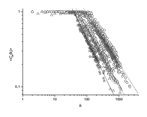
Figure 6: Mean clustering coefficient $\langle C_{\mathds{P}}(k)\rangle$ of several PTN in $\mathds{P}$-space. Berlin (stars), London (triangles), Taipei (circles).

The connectivity within the closest neighborhood of a given node is described by the clustering coefficient defined as

$$C_{i}=\frac{2y_{i}}{k_{i}(k_{i}-1)},$$ (6)

where $y_{i}$ is the number of links between the $k_{i}$ nearest neighbors of the node $i$. The clustering coefficient of a node may also be defined as the probability of any two of its randomly chosen neighbors to be connected. For the mean value of the clustering coefficient of a random graph one finds

$$\langle C\rangle^{\cal R}=\frac{\langle k\rangle^{\cal R}}{N}=\frac{2M}{N^{2}}.$$ (7)

In Table 2 we give the values of the mean clustering coefficient in ${\mathds{L}}$, ${\mathds{P}}$, and ${\mathds{C}}$-spaces. The highest absolute values of the clustering coefficient are found in ${\mathds{P}}$-space, where their range is given by $\langle C_{\mathds{P}}\rangle=0.7\div 0.9$ (c.f. with $\langle C_{\mathds{L}}\rangle=0.02\div 0.1$). This is due to the fact that in this space each route gives rise to a fully connected subgraph (complete graph). In order to make numbers comparable we normalize the value of $\langle C\rangle$ by the mean clustering coefficient (7) of a random graph of the same size:

$$c=N^{2}\langle C\rangle/(2M).$$ (8)

In $\mathds{L}$ and $\mathds{P}$-representations we find the mean clustering coefficient to be larger by orders of magnitude relative to the random graph. This difference is less pronounced in ${\mathds{C}}$-space indicating a lower degree of organization in these networks. Furthermore, we find these values to vary strongly within the sample of the 14 cities. This suggests that the concepts according to which various PTNs are structured lead to a measurable difference in their organization.

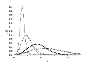
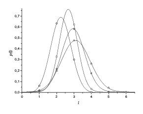
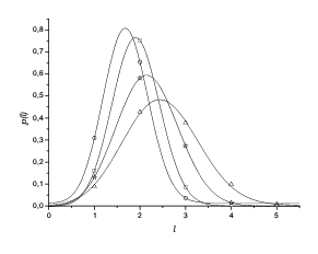
a                                                     b                                                     c

Figure 7: Mean shortest path length distribution $P(\ell)$ for the PTN of Berlin (stars), Hong Kong (circles), Paris (boxes) and Rome (triangles). Solid line shows a fit to the function (12). a: $\mathds{L}$-space; b: $\mathds{P}$-space; c: $\mathds{C}$-space.

In $\mathds{P}$-space the clustering coefficient of a node is strongly correlated with the node degree. In Fig. 6 we show the mean clustering coefficient of nodes of degree $k$, $\langle C_{\mathds{P}}(k)\rangle$, as a function of $k$ for several PTNs. Its behavior can be understood as follows. Recall that the $\mathds{P}$-space the degree of a node (station) equals the number of stations that can be reached from a given one. Each route enters the network as a complete graph, within which every node has a clustering coefficient of one. A small number $k$ of neighbors of a given station indicates that the station belongs to a single route (i.e. $\langle C_{\mathds{P}}(k)\rangle$ is most probably equal to one). For nodes with higher degrees $k$ it is more probable that they belong to more than one route. Consequently, $\langle C_{\mathds{P}}(k)\rangle$ decreases with $k$. The change in the behavior of $\langle C_{\mathds{P}}(k)\rangle$ should occur at some value of $k$ which is of the order of the mean number of stops of the routes. The prominent feature of the function $\langle C_{\mathds{P}}(k)\rangle$ in $\mathds{P}$-space is that it decays following a power law

$$\langle C_{\mathds{P}}(k)\rangle\sim~{}k^{-\beta}.$$ (9)

Within a simple model of networks with star-like topology this exponent is found to be of value $\beta=1$ Sienkiewicz05 . In transport networks. This behavior was first observed for the Indian railway network Sen03 and then for the Polish PTNs Sienkiewicz05 . In our case, the values of the exponent $\beta$ for the networks studied lie in the range from $0.65$ (Saõ Paolo) to $0.96$ (Los Angeles) with a mean value of $0.82$.

IV Global characteristics

IV.1 Path length distribution

Let $\ell_{i,j}$ be the length of a shortest path between sites $i$ and $j$ in a given space. The mean shortest path is defined as

$$\langle\ell\rangle=\frac{2}{N(N-1)}\sum_{i>j=1}^{N}\ell_{ij}.$$ (10)

Note that $\langle\ell\rangle$ is well-defined only if nodes $i$ and $j$ belong to the same connected component of the network. In the following any expression as given in Eq. (10) will be restricted to this case. Furthermore, related network characteristics will be calculated for the largest (or giant) connected component, GCC. Correspondingly, $N$ denotes the number of constituting nodes of this component. Denoting the path length distribution as $P(\ell)$, the average (10) reads

$$\langle\ell\rangle=\sum_{\ell=1}^{\ell^{\rm max}}P(\ell)\ell,$$ (11)

where $\ell^{\rm max}$ is maximal shortest path length found on the connected component. In Fig. 7 we plot the mean shortest path length distributions obtained in different spaces for several selected cities. Together with the data we plot a fit to the asymmetric unimodal distribution Sienkiewicz05 :

$$P(\ell)=A\ell\exp{(-B\ell^{2}+C\ell)},$$ (12)

where $A,B,C$ are fit parameters. As can be seen from the figures, the data is generally nicely reproduced by this ansatz. However, in certain networks additional features may lead to a deviation from this behavior as can be seen from Fig. 8,

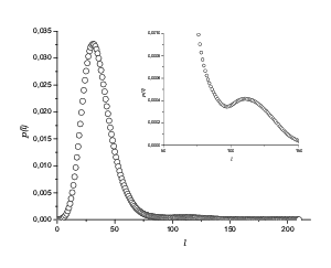
Figure 8: Mean shortest path length distribution in $\mathds{L}$-space, $P_{\mathds{L}}(\ell)$, for the PTN of Los Angeles.

which shows the mean shortest path length distribution in $\mathds{L}$-space $P_{\mathds{L}}(\ell)$ for Los Angeles. One observes a second local maximum on the right shoulder of the distribution. Qualitatively this behavior may be explained by assuming that the PTN consists of more than one community. For the simple case of one large community and a second smaller one at some distance this situation will result in short intra-community paths which will give rise to a global maximum and a set of longer paths that connect the larger to the smaller community resulting in additional local maxima. Such a situation definitely appears to be present in the case of the Los Angeles PTN, see Fig. 1.

Let us introduce a characteristic that informs how remote a given node is from the other nodes of the networks. For the node $i$ this may be characterized by the value:

$$\ell_{i}=\frac{1}{N-1}\sum_{j\neq i}\ell_{ij}.$$ (13)

Now, the mean shortest path (10) can be defined in terms of $\ell_{i}$ as:

$$\langle\ell\rangle=\frac{1}{N}\sum_{i}\ell_{i}.$$ (14)

In order to look for correlations between $\ell_{i}$ and the node degree $k_{i}$ let us introduce the value:

$$\ell(k)=\frac{1}{N_{k}}\sum_{i=1}^{N}\ell_{i}\delta_{k,k_{i}},$$ (15)

where $N_{k}$ is number of nodes of degree $k$ and $\delta_{k,k_{i}}$ is the Kronecker delta. Consequently, $\ell(k)$ is the mean shortest path length between any node of degree $k$ and other nodes of the network. For the majority of the analyzed cities the dependence of the mean path $\ell_{\mathds{L}}(k)$ (15) on the node degree $k$ in $\mathds{L}$-space can be approximated by a power law

$$\ell_{\mathds{L}}(k)\sim k^{-\alpha_{\mathds{L}}}.$$ (16)

The value of the exponent varies in the range $\alpha_{\mathds{L}}=0.17\div 0.27$. We show this dependence for several cities in Fig. 9.

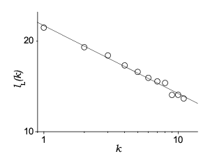
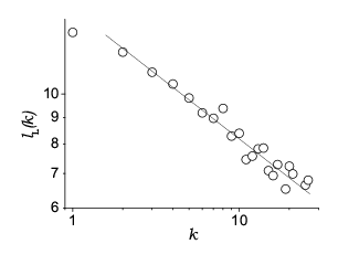
a                                         b

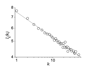
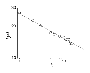
c                                         d

Figure 9: Mean path $\ell_{\mathds{L}}(k)$ (15) in the ${\mathds{L}}$-space as a function of the node degree $k$ with a fit to the power law decay (16). a: Berlin, $\alpha_{\mathds{L}}=0.23$; b: Hong Kong, $\alpha_{\mathds{L}}=0.25$; c: Paris, $\alpha_{\mathds{L}}=0.15$; d: Taipei, $\alpha_{\mathds{L}}=0.23$.

A particular relation between path lengths and node degrees can be shown to hold relating the mean path length between two nodes to the product of their node degrees. To this end let us define

$$\ell(k,q)=\sum_{i,j=1}^{N}\ell_{i,j}\delta_{k_{i}k_{j},kq}.$$ (17)

As has been shown in Holyst05 , this relation can be approximated by

$$\ell(k,q)=A-B\log(kq).$$ (18)

For random networks the coefficients $A$ and $B$ can be calculated exactly Fronczak03 . The validity of Eq. (18) was checked on the base of PTNs of some Polish cities and a rather good agreement for the majority of the cities was found in ${\mathds{L}}$-space. In our analysis which concerns PTNs of much larger size, we do not observe the same good agreement for all cities. The suggested logarithmic dependence (18) was found by us in ${\mathds{L}}$-space also for the larger cities, however with much more pronounced scatter of data for large values of the product $kq$. In Fig. 10 we plot the mean path $\ell_{\mathds{L}}(k,q)$ in the ${\mathds{L}}$-space for the PTN of Berlin, Hong Kong, Rome, and Taipei. Note, however, that due to the scatter of data a logarithmic dependence frequently is indistinguishable from a power law with a small exponent.

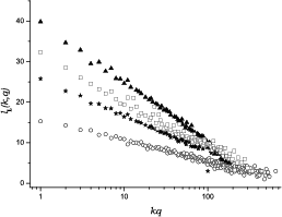
Figure 10: Mean path $\ell_{\mathds{L}}(k,q)$ (17) in the $\mathds{L}$-space as a function of $kq$ for the PTN of Berlin (stars), Hong Kong (circles), Rome (triangles), and Taipei (squares).

In $\mathds{P}$-space, the shortest path length $\ell_{ij}$ gives the minimal number of routes required to be used in order to reach site $j$ starting from the site $i$. In turn, $\ell_{i}$, Eq. (13), defines the number of routes one uses on average traveling from the site $i$ to any node of the network. The higher the node degree, the easier it is to access other routes in the network. Therefore, also in $\mathds{P}$-space one expects a decrease of $\ell_{\mathds{P}}(k)$ when $k$ increases. This is shown for several cities in Fig. 11. Besides the expected decrease of $\ell_{\mathds{P}}(k)$, one can see a tendency to a power-law decay

$$\ell_{\mathds{P}}(k)\sim k^{-\alpha_{\mathds{P}}}.$$ (19)

The value of the exponent $\alpha_{\mathds{P}}$ varies in the interval $\alpha_{\mathds{P}}=0.09$ (for Sydney) to $\alpha_{\mathds{P}}=0.17$ (for Dallas) and is centered around $\alpha_{\mathds{P}}=0.12\div 0.13$ as shown for the cities in Fig. 11. The mean path $\ell_{\mathds{P}}(k,q)$ as a function of $kq$ for several cities is given in ${\mathds{P}}$-space in Fig. 12. The scattering of data is much more pronounced than in $\mathds{L}$-space. However one distinguishes a tendency of $\ell_{\mathds{P}}(k,q)$ to decrease with an increase of $kq$. The red lines in Figs. 12 are the guides to the eye characterizing the decay.

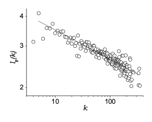
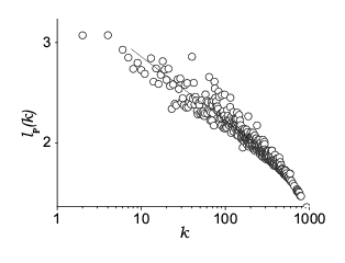
a                                         b

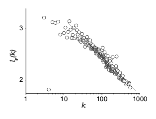
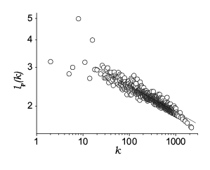
c                                         d

Figure 11: Mean path $\ell_{\mathds{P}}(k)$ in $\mathds{P}$-space as a function of the node degree $k$ and its fit to the power law decay (19). a: Berlin, $\alpha_{\mathds{P}}=0.13$; b: Hong Kong, $\alpha_{\mathds{P}}=0.12$; c: Paris, $\alpha_{\mathds{P}}=0.13$; d: Taipei, $\alpha_{\mathds{L}}=0.12$.

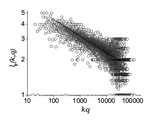
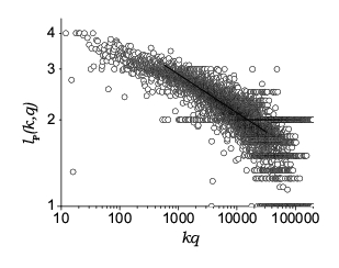
a                                         b

Figure 12: Mean path $\ell_{\mathds{P}}(k,q)$ in $\mathds{P}$-space for PTN of Berlin (a) and Paris (b) as a function of $kq$.

IV.2 Centralities

To measure the importance of a given node with respect to different properties of a graph a number of so-called centrality measures have been introduced Brandes01 ; Sabidussi66 ; Hage95 ; Shimbel53 ; Freeman77 . Most of them are based on either measuring path lengths to other nodes or on counting the number of paths between other nodes mediated by this node. The closeness ${\cal C}^{c}(i)$ Sabidussi66 and graph ${\cal C}^{g}(i)$ Hage95 centralities of a node $i$ are based on the shortest path lengths $\ell_{ij}$ to other nodes $j$:

$${\cal C}^{c}(i) = \frac{1}{\sum_{j\neq i}\ell_{i,j}},$$ (20)

$${\cal C}^{g}(i) = \frac{1}{{\rm max}_{j\neq i}\ell_{i,j}}.$$ (21)

Only nodes $j$ that belong to the same connected component as $i$ contribute to (20), (21). For a given node these properties obviously depend on the size of the connected component to which the node belongs. The importance of the node $i$ with respect to the connectivity within the graph may be measured in terms of the number of shortest paths $\sigma_{jk}(i)$ between nodes $j$ and $k$ that go via node $i$. Denoting by $\sigma_{jk}$ the overall number of shortest paths between nodes $j$ and $k$ one defines stress ${\cal C}^{s}(i)$ Shimbel53 and betweenness ${\cal C}^{b}(i)$ Freeman77 centralities by:

$${\cal C}^{s}(i) = \sum_{j\neq i\neq k}\sigma_{jk}(i),$$ (22)

$${\cal C}^{b}(i) = \sum_{j\neq i\neq k}\frac{\sigma_{jk}(i)}{\sigma_{jk}}.$$ (23)

Numerical values of the betweenness centrality (23) are given in Table 1 in $\mathds{L}$, $\mathds{P}$ and $\mathds{C}$-spaces.

Averaging the two centralities that are based on path length (20), (21) one obtains values that are closely related to the average shortest path length on the GCC. As far as this relation is independent of the representation of the PTN, we find very similar correspondence between $\langle\ell\rangle$ and the mean centralities $\langle{\cal C}^{c}\rangle$, $\langle{\cal C}^{g}\rangle$ in all spaces considered as shown in Fig. 13. The fact that these centralities are based on the inverse path length is reflected by the negative slope of the curves shown in the figures.

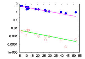
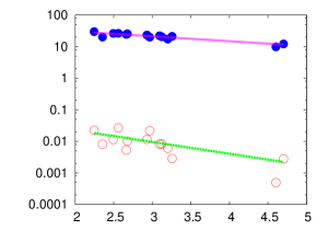
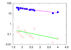
a                                                     b                                                     c

Figure 13: Correspondence between the mean shortest path $\langle\ell\rangle$ and mean centralities $\langle{\cal C}^{c}\rangle$ (open circles), $\langle{\cal C}^{g}\rangle$ (filled circles) for all fourteen PTN listed in Table 2 in (a) $\mathds{L}$, (b) $\mathds{P}$, and (c) $\mathds{C}$-spaces.

The betweenness centrality (23) and the related stress centrality (22) of a given node measure the share of the mean paths between nodes that are mediated by that node. It is obvious that a node with a high degree has a higher probability to be part of any path connecting other nodes. This relation between ${\cal C}^{b}$ and the node degree may be quantified by observing their correlation. In Figs. 14 we plot the mean betweenness centrality $\langle{\cal C}^{b}(k)\rangle$ of all nodes that have a given degree $k$. There, we present results for the PTN of Paris in $\mathds{L}$, $\mathds{C}$ and $\mathds{P}$, and $\mathds{B}$-spaces. Especially well expressed is the betweenness-degree correlation in $\mathds{L}$-space (Fig. 14a) and with somewhat less precision in $\mathds{C}$-space (Fig. 14b). In both cases there is a clear tendency to a power law $\langle{\cal C}^{b}(k)\rangle\sim k^{\eta}$ with an exponent $\eta=2\div 3$. Let us note here, that this power law together with the scale free behavior of the degree distribution implies that also the betweenness distribution should follow a power law with an exponent $\delta$. This behavior is clearly identified in Fig.15 for the $\mathds{L}$-space betweenness distribution of the Paris PTN, for which we find an exponent $\delta\approx 1.5$. The resulting scaling relation Goh01

$$\eta=(\gamma-1)/(\delta-1)$$ (24)

is fulfilled within the accuracy for these exponents. In the plots for both $\mathds{B}$ and $\mathds{P}$-spaces we observe the occurrence of two regimes which correspond to small and large degrees $k$. This separation however has a different origin in each of these cases. In the $\mathds{B}$-space representation, the network consists of nodes of two types, route nodes and station nodes. Typically, station nodes are connected only to a low number of routes while there is a minimal number of stations per route. One may thus identify the low degree behavior as describing the betweenness of station nodes, while the high degree behavior corresponds to that of route nodes. In the overlap region of the two regimes one may observe that when having the same degree station nodes have a higher betweenness than route nodes. The occurrence of two regimes in the $\mathds{P}$-space representation has a similar origin as the change of behavior observed for the mean clustering coefficient $\langle C_{\mathds{P}}(k)\rangle$, see Fig.6. Namely, stations with low degrees in general belong only to a single route and thus are of low importance for the connectivity within the network resulting in a low betweenness centrality. Comparing our results with those of Ref. Sienkiewicz05 we do not however find a saturation for the low $k$ region, as observed there. Similar betweenness $\langle{\cal C}^{b}(k)\rangle$ - degree relations as observed in Fig. 14 for the PTN of Paris we also find for most of the other cities, however, with different quality of expression.

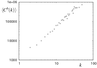
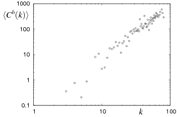
a                                               b

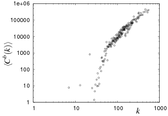
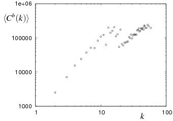
c                                               d

Figure 14: Mean betweenness centrality $\langle{\cal C}^{b}(k)\rangle$ - degree $k$ correlations for the PTN of Paris in (a) $\mathds{L}$, (b) $\mathds{C}$, (c) $\mathds{P}$, and (d) $\mathds{B}$-spaces.

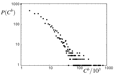
Figure 15: Betweenness centrality ${\cal C}^{b}$ - distribution for PTN of Paris in $\mathds{L}$ - space.

IV.3 Harness

Besides the local and global properties of networks described above which can be defined in any type of network, there are some characteristics that are unique for PTNs and networks with similar construction principles. A particularly striking example is the fact that as far as the routes share the same grid of streets and tracks often a number of routes will proceed in parallel along shorter or longer sequences of stations. Similar phenomena are observed in networks built with real space consuming links such as cables, pipes, neurons, etc. In the present case this behavior may be easily worked out on the basis of sequences of stations serviced by each route. To quantify this behavior recently the notion of network harness has been introduced Ferber07a . It is described by the harness distribution $P(r,s)$: the number of sequences of $s$ consecutive stations that are serviced by $r$ parallel routes. Similarly to the node-degree distributions, we observe that the harness distribution for some cities (Hong Kong, Istanbul, Paris, Rome, Saõ Paolo, Sydney) may be fitted by a power law:

$$P(r,s)\sim r^{-\gamma_{s}},\hskip 20.00003pt\mbox{for fixed $s$},$$ (25)

whereas the PTNs of other cities (Berlin, Dallas, Düsseldorf, London, Moscow) are better fitted to an exponential decay:

$$P(r,s)\sim\exp{(-r/\hat{r}_{s})},\hskip 20.00003pt\mbox{for fixed $s$}.$$ (26)

As examples we show the harness distribution for Istanbul (Fig. 16a) and for Moscow (Fig. 16b). Moreover, sometimes (we observe this for Los Angeles and Taipei), for larger $s$ the regime (25) changes to (26). We show this for the PTN of Los Angeles in Fig. 17. There, one can see that for small values of $s$ the curves are better fitted to a power law dependence (25). With increasing $s$ a tendency to an exponential decay (26) appears: Fig. 17b.

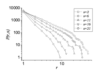
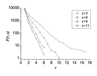
a                                                     b

Figure 16: Cumulative harness distributions for Istanbul (a) and for Moscow (b) PTN.

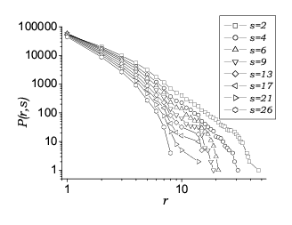
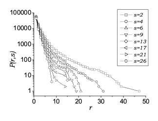
a                                               b

Figure 17: Cumulative harness distributions for Los Angeles. a: log-log scale; b: log-linear scale.

As one can observe from the Figs. 16, 17 the slope of the harness distribution $P(r,s)$ as a function of the number of routes $r$ increases with an increase of the sequence length $s$. For PTNs for which the harness distribution follows power law (25) the corresponding exponents $\gamma_{s}$ are found in the range of $\gamma_{s}=2\div 4$. For those distributions with an exponential decay the scale $\hat{r}_{s}$ (26) varies in the range $\hat{r}_{s}=1.5\div 4$. The power laws observed for the behavior of $P(r,s)$ indicate a certain level of organization and planning which may be driven by the need to minimize the costs of infrastructure and secondly by the fact that points of interest tend to be clustered in certain locations of a city. Note that this effect may be seen as a result of the strong interdependence of the evolutions of both the city and its PTN.

We want to emphasize that the harness effect is a feature of the network given in terms of its routes but it is invisible in any of the graph representations presented so far. In particular PTN representation in terms of a simple graph which do not contain multiple links (such as $\mathds{L}$, $\mathds{P}$, $\mathds{C}$ and $\mathds{B}$-spaces) can not be used to extract harness behavior. Furthermore, the multi-graph representations (such as $\mathds{L}^{\prime}$, $\mathds{P}^{\prime}$, and $\mathds{C}^{\prime}$-spaces) would need to be extended to account for the continuity of routes. As noted above, the notion of harness may be useful also for the description of other networks with similar properties. On the one hand, the harness distribution is closely related to distributions of flow and load on the network. On the other hand, in the situation of space-consuming links (such as tracks, cables, neurons, pipes, vessels) the information about the harness behavior may be important with respect to the spatial optimization of networks.

A generalization may be readily formulated to account for real-world networks in which links (such as cables) are organized in parallel over a certain spatial distance. While for the PTN this distance is simply measured by the length of a sequence of stations, a more general measure would be the length of the contour along which these links proceed in parallel.

V Generalized assortativities

To describe correlations between the properties of neighboring nodes in a network the notion of assortativity was introduced measuring the correlation between the node degrees of neighboring nodes in terms of the mean Pearson correlation coefficient Newman02 ; Newman03b . Here, we propose to generalize this concept to also measure correlations between the values of other node characteristics (other observables). For any link $i$ let $X_{i}$ and $Y_{i}$ be the values of the observable at the two nodes connected by this link. Then the correlation coefficient is given by:

$$r=\frac{M^{-1}\sum_{i}X_{i}Y_{i}-[M^{-1}\sum_{i}\frac{1}{2}(X_{i}+Y_{i})]^{2}}{M^{-1}\sum_{i}\frac{1}{2}(X_{i}^{2}+Y_{i}^{2})-[M^{-1}\sum_{i}\frac{1}{2}(X_{i}+Y_{i})]^{2}}$$ (27)

where summation is performed with respect to the $M$ links of the network. Taking $X_{i}$ and $Y_{i}$ to be the node degrees Eq. (27) is equivalent to the usual formula for the assortativity of a network Newman02 . Here we will call this special case the degree assortativity $r^{(1)}$. In the following we will investigate correlations between other network characteristics such as the observables considered above, $z_{2}$, $C_{i}$ (6), ${\cal C}^{c}$ (20), ${\cal C}^{g}$ (21), ${\cal C}^{s}$ (22), ${\cal C}^{b}$ (23). Consequently, this results in generalized assortativities of next nearest neighbors ($r^{(2)}$), clustering coefficients ($r^{cl}$), closeness ($r^{c}$), graph ($r^{g}$), stress ($r^{s}$), and betweenness ($r^{b}$) centralities.

The numerical values of the above introduced assortativities $r^{(1)}$ and $r^{(2)}$ for the PTN under discussion are listed in Table 4 in $\mathds{L}$, $\mathds{P}$ and $\mathds{C}$-spaces. With respect to the values of the standard node degree assortativity $r^{(1)}_{\mathds{L}}$ in $\mathds{L}$-space, we find two groups of cities. The first is characterized by values $r^{(1)}_{\mathds{L}}=0.1\div 0.3$. Although these values are still small they signal a finite preference for assortative mixing. That is, links tend to connect nodes of similar degree. In the second group of cities these values are very small $r^{(1)}_{\mathds{L}}=-0.02\div 0.08$ showing no preference in linkage between nodes with respect to node degrees. PTNs of both large and medium sizes are present in each of the groups. This indicates the absence of correlations between network size and degree assortativity $r^{(1)}_{\mathds{L}}$ in $\mathds{L}$-space. Measuring the same quantity in the $\mathds{P}$ and $\mathds{C}$-spaces, we observe different behavior. In $\mathds{P}$-space almost all cities are characterized by very small (positive or negative) values of $r^{(1)}_{\mathds{P}}$ with the exception of the PTNs of Istanbul ($r^{(1)}_{\mathds{P}}=-0.12$) and Los Angeles ($r^{(1)}_{\mathds{P}}=0.12$). On the contrary, in $\mathds{C}$-space PTNs demonstrate clear assortative mixing with $r^{(1)}_{\mathds{C}}=0.1\div 0.5$. An exception is the PTN of Paris with $r^{(1)}_{\mathds{C}}=0.06$.

City	$r_{\mathds{L}}^{(1)}$	$r_{\mathds{L}}^{(2)}$	$r_{\mathds{P}}^{(1)}$	$r_{\mathds{P}}^{(2)}$	$r_{\mathds{C}}^{(1)}$	$r_{\mathds{C}}^{(2)}$
Berlin	0.158	0.616	0.065	0.441	0.086	0.318
Dallas	0.150	0.712	0.154	0.728	0.290	0.550
Düsseldorf	0.083	0.650	0.041	0.494	0.244	0.180
Hamburg	0.297	0.697	0.087	0.551	0.246	0.605
Hong Kong	0.205	0.632	-0.067	0.238	0.131	0.087
Istanbul	0.176	0.726	-0.124	0.378	0.282	0.505
London	0.221	0.589	0.090	0.470	0.395	0.620
Los Angeles	0.240	0.728	0.124	0.500	0.465	0.753
Moscow	0.002	0.312	-0.041	0.296	0.208	0.011
Paris	0.064	0.344	-0.010	0.258	0.060	-0.008
Rome	0.237	0.719	0.044	0.525	0.384	0.619
Saõ Paolo	-0.018	0.437	-0.047	0.266	0.211	0.418
Sydney	0.154	0.642	0.077	0.608	0.458	0.424
Taipei	0.270	0.721	0.009	0.328	0.100	0.041

Table 4: Nearest neighbors and next nearest neighbors assortativities $r^{(1)}$ and $r^{(2)}$ in different spaces for the whole PTN.

As we have seen above, the PTNs demonstrate assortative ($r^{(1)}>0$) or neutral ($r^{(1)}\sim 0$) mixing with respect to the node degree (first nearest neighbors number) $k$. Calculating assortativity with respect to the second next nearest neighbor number $r^{(2)}$ we explore the correlation of a wider environment of adjacent nodes. Due to the fact that in this case the two connected nodes share at least part of this environment (the first nearest neighbors of a node form part of the second nearest neighbors of the adjacent node) one may expect the assortativity $r^{(2)}$ to be non-negative. Results for $r^{(2)}$ shown in Table 4 appear to confirm this assumption. In all the spaces considered, we find that all PTNs that belong to the group of neutral mixing with respect to $k$ also belong to the same group with respect to the second nearest neighbors. For those PTNs that display significant nearest neighbors assortativity $r^{(1)}$ we find that the second nearest neighbor assortativity $r^{(2)}$ is in general even stronger in line with the above reasoning.

Recall that both closeness and graph centralities ${\cal C}^{c}$ and ${\cal C}^{g}$ are measured in terms of path lengths, Eqs. (20), (21). It is natural to expect that adjacent nodes will have very similar (or almost identical) centralities ${\cal C}^{c}$ and ${\cal C}^{g}$. In turn this will lead to strong assortative mixing with high assortativities $r^{c}$ and $r^{g}$. This assumption holds only if the average path length in the network is sufficiently large. The latter is certainly the case for PTNs in $\mathds{L}$-space but it does not hold in $\mathds{P}$ and even less in $\mathds{C}$-spaces. Indeed, in $\mathds{L}$-space, where most PTNs display a mean path length $\langle\ell_{\mathds{L}}\rangle>10$ (see Table 2) we find values of $r^{c}_{\mathds{L}}$ in the range $r^{c}_{\mathds{L}}=0.904\div 0.998$ ($r^{g}_{\mathds{L}}=0.914\div 0.999$). Exceptions are the two PTNs of cities with the smallest mean paths. These are Moscow ($r^{c}_{\mathds{L}}=0.865$, $r^{g}_{\mathds{L}}=0.870$) with $\langle\ell_{\mathds{L}}\rangle=7.0$ and Paris ($r^{c}_{\mathds{L}}=0.831$, $r^{g}_{\mathds{L}}=0.800$) with $\langle\ell_{\mathds{L}}\rangle=6.4$.

In $\mathds{P}$ and $\mathds{C}$-spaces where the mean path lengths are much shorter (of the order of three in $\mathds{P}$ and of the order of two in $\mathds{C}$-spaces) the one-step difference in path length between adjacent nodes leads to much reduced assortative mixing. Numerically this is reflected in much lower (however positive) values of corresponding assortativities for PTNs where $\langle\ell\rangle$ is especially small. Indeed, for all PTNs that display in ${\mathds{P}}$-space a mean path length $\langle\ell_{\mathds{P}}\rangle<2.7$ we find $r^{c}_{\mathds{P}}<0.5$ ($r^{g}_{\mathds{P}}<0.4$). At the same time, PTNs with larger $\langle\ell_{\mathds{P}}\rangle$ may display larger assortativities even in ${\mathds{P}}$-space. The extreme example is Los Angeles with $\langle\ell_{\mathds{P}}\rangle=4.3$ and $r^{c}_{\mathds{P}}=0.914$, $r^{g}_{\mathds{P}}=0.844$. In $\mathds{C}$-space, where vertices are routes the mean path length is even smaller and further reduction of closeness and graph centrality assortativities is observed. For five PTNs we find in $\mathds{C}$-space $\langle\ell_{\mathds{C}}\rangle<2$ (see Table 2) and for these $r^{c}_{\mathds{C}}<0.3$, $r^{g}_{\mathds{C}}<0.3$. Again the largest values are attained in the Los Angeles PTN with $\langle\ell_{\mathds{C}}\rangle=3.4$ and $r^{c}_{\mathds{C}}=0.828$, $r^{g}_{\mathds{C}}=0.648$.

For the other generalized assortativities (stress and betweenness centrality assortativities $r^{s}$ and $r^{b}$ and clustering coefficient assortativity $r^{cl}$ we in general find no evidence for any (positive or negative) correlation in any of the spaces considered. The only exception are the stress and betweenness centrality assortativities in ${\mathds{L}}$-space, $r^{s}_{\mathds{L}}$ and $r^{b}_{\mathds{L}}$. There, small but significantly positive values of $r^{s}_{\mathds{L}}$ and $r^{b}_{\mathds{L}}$ are found. The latter is explained by the relatively large mean path length in this space in conjunction with relatively small node degree values. Let us recall that stress and betweenness centralities essentially count the number of shortest paths mediated by a given node. If a selected node is a part of many such long paths while having low degree, there is high probability that any of its neighbors will also be a part of these paths. Consequently, a positive value of $r^{c}$ ($r^{g}$) will arise. The analogous conclusion can be drawn for nodes with low betweenness (or stress) centralities. For most PTNs the values of the assortativities under consideration change in the range $r^{s}_{\mathds{L}}=0.26\div 0.64$, $r^{b}_{\mathds{L}}=0.20\div 0.61$. Exceptions are the PTNs which in ${\mathds{L}}$-space have mean path length $\langle\ell_{\mathds{L}}\rangle<10$, namely Moscow, Paris and Saõ Paolo. There we find $r^{s}_{\mathds{L}}=0.02\div 0.10$, $r^{b}_{\mathds{L}}=0.02\div 0.10$.

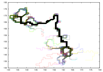
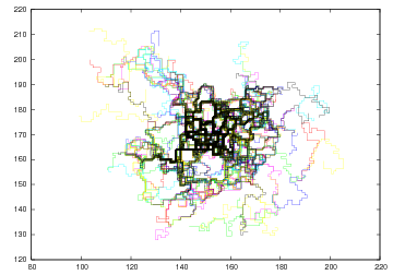
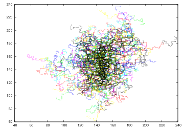
$b=0.1$                                             $b=0.2$                                             $b=0.5$

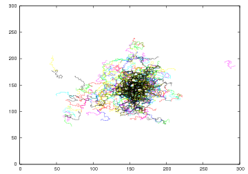
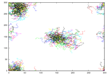
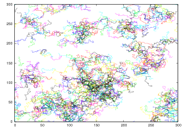
$a=15$                                             $a=20$                                             $a=500$

Figure 18: PTN maps of different simulated cities of size $300\times 300$ with $R=1024$ routes of $S=64$ stations each (color online). First row: $a=0$, $b=0.1\div 0.5$. Second row: $b=0.5$, $a=15\div 500$. With an increase of $b$ routes cover more and more area. Increase of $a$ leads to clusterisation of the network.

VI Modeling PTNs

VI.1 Motivation and description of the model

Having at hand the above described wealth of empirical data and analysis with respect to typical scenarios found in a variety of real-world PTNs we feel in the position to propose a model that albeit being simple may capture the characteristic features of these networks. Nonetheless it should be capable of discriminating between some of the various scenarios observed.

If we were only to reproduce the degree distribution of the network, standard models such as random networks Dorogovtsev03 ; Newman01a or preferential attachment type models prefattach ; Amaral00 ; Liu02 ; Newman01b ; Li03 ; Ramasco04 would suffice. The evolution of such networks however is based on the attachment of nodes. For description of PTNs the concept of routes as finite sequences of stations is essential Holovatch06 ; Angeloudis06 ; Ferber07a ; Ferber07b and allows for the representation with respect to the spaces defined above. Moreover, taking a route as the essential element of PTN growth allows to account for the essential bipartite structure of this network Seaton04 ; Zhang06 ; Guillaume06 ; Chang07 . Therefore, the growth dynamics in terms of routes will be a central ingredient of our model. Another obvious requirement is the embedding of this model in two-dimensional space. To simplify matters we will restrict the model to a two-dimensional grid, in particular to square lattice. Both the observations of power law degree distributions as well as the occurrence of the corresponding harness distributions described above indicate a preference of routes to service common stations (i.e. an attraction between routes).

Let us describe our model in more detail. As noticed above, a route will be modeled as a sequence of stations that are adjacent nodes on a two-dimensional square lattice. Noting that in general loops in PTN routes are almost absent, a most simple choice to model a PTN route is a self-avoiding walk (SAW). It may sound less obvious that a route apart from being non self-intersecting proceeds randomly. However, the analysis of geographical data Ferber07a has shown that the fractal dimension of PTN routes closely coincides with that of a two-dimensional SAW, $d_{f}=4/3$ Nienhuis82 . To incorporate all the above features the model is set up as follows. A model PTN consists of $R$ routes of $S$ stations each constructed on a possibly periodic $X\times X$ square lattice. The dynamics of the route generation adheres to the following rules:

• 1. Construct the first route as a SAW of $S$ lattice sites.

• 2. Construct the $R-1$ subsequent routes as SAWs with the following preferential attachment rules:

  a) choose a terminal station at $\vec{x}_{0}$ with probability

  $$p\sim k_{\vec{x}_{0}}+a/X^{2};$$ (28)

  b) choose any subsequent station $\vec{x}$ of the route with probability

  $$p\sim k_{\vec{x}}+b.$$ (29)

In (28), (29) $k_{\vec{x}}$ is the number of times the lattice site $\vec{x}$ has been visited before (the number of routes that pass through $\vec{x}$). Note that to ensure the SAW property any route that intersects itself is discarded and its construction is restarted with step 2a).

$R$	$S$	$b$	$\langle k_{\mathds{L}}\rangle$	$z_{\mathds{L}}$	$\ell_{\mathds{L}}^{\rm max}$	$\langle\ell_{\mathds{L}}\rangle$	$\langle{\cal C_{\mathds{L}}}^{b}\rangle$	$\langle k_{\mathds{P}}\rangle$	$z_{\mathds{P}}$	$\ell_{\mathds{P}}^{\rm max}$	$\langle\ell_{\mathds{P}}\rangle$	$\langle{\cal C_{\mathds{P}}}^{b}\rangle$	$c_{\mathds{P}}$	$\langle k_{\mathds{C}}\rangle$	$z_{\mathds{C}}$	$\ell_{\mathds{C}}^{\rm max}$	$\langle\ell_{\mathds{C}}\rangle$	$\langle{\cal C_{\mathds{C}}}^{b}\rangle$	$c_{\mathds{C}}$
256	16	0.5	2.92	1.66	61	20.8	4.7$\times 10^{3}$	44.15	3.18	7	3.0	4.7$\times 10^{2}$	7.98	86.39	1.36	6	1.9	1.2$\times 10^{2}$	2.22
256	16	5.0	2.99	1.74	80	21.7	7.5$\times 10^{3}$	42.95	3.76	9	3.4	8.8$\times 10^{2}$	11.7	59.96	1.99	8	2.2	1.5$\times 10^{2}$	2.79
256	32	0.5	2.76	1.60	127	38.1	3.0$\times 10^{4}$	84.45	4.32	8	3.3	1.9$\times 10^{3}$	13.6	60.51	1.75	7	2.2	1.6$\times 10^{2}$	2.90
256	32	5.0	2.90	1.72	177	43.1	5.3$\times 10^{4}$	74.24	5.22	10	4.0	3.8$\times 10^{3}$	23.7	33.06	2.69	9	2.8	2.3$\times 10^{2}$	4.55
512	16	0.5	2.95	1.68	73	22.5	6.7$\times 10^{3}$	50.07	3.39	7	3.1	6.5$\times 10^{2}$	9.14	169.7	1.44	6	1.9	2.3$\times 10^{2}$	2.25
512	16	5.0	3.12	1.78	80	23.3	1.0$\times 10^{4}$	51.56	3.79	10	3.5	1.2$\times 10^{3}$	12.3	115.3	2.24	9	2.1	2.9$\times 10^{2}$	2.88
512	32	0.5	2.83	1.63	166	44.2	4.7$\times 10^{4}$	99.53	4.56	10	3.6	2.8$\times 10^{3}$	15.7	118.4	2.03	9	2.2	3.0$\times 10^{2}$	2.92
512	32	5.0	3.12	1.79	175	44.6	7.2$\times 10^{4}$	97.05	5.37	9	3.9	4.7$\times 10^{3}$	22.2	60.36	3.08	8	2.7	4.4$\times 10^{2}$	5.04
1024	64	0.5	2.86	1.66	325	80.7	3.3$\times 10^{5}$	242.2	6.32	9	3.7	1.1$\times 10^{4}$	23.4	213.3	2.42	8	2.2	6.1$\times 10^{2}$	3.10
1024	64	1.0	2.97	1.72	355	88.5	4.8$\times 10^{5}$	222.2	6.74	12	4.2	1.7$\times 10^{4}$	32.4	143.9	2.97	11	2.5	7.9$\times 10^{2}$	4.39

Table 5: Characteristics of the simulated PTN with $X=300$, $a=0$ for different parameters $R$, $S$, and $b$. The rest of notations as in Table 2.

VI.2 Global topology of model PTN

Let us first investigate the global topology of this model as function of its parameters. We first fix both the number of routes $R$ and the number of stations $S$ per route as well as the size of the lattice $X$. This leaves us with essentially two parameters $a$ and $b$, Eqs. (28), (29). Dependencies on $R$, $S$, and $X$ will be studied below.

For the real-world PTNs as studied in the previous sections, almost all stations belong to a single component, GCC, with the possible exception of a very small number of routes. Within the network however we often observe what above we called the harness effect of several routes proceeding in parallel for a sequence of stations. Let us first investigate from a global point of view which parameters $a$ and $b$ reproduce realistic maps of PTNs. In Fig. 18 we show simulated PTNs on lattices $300\times 300$ for $R=1024$, $S=64$ and different values of the parameters $a$ and $b$. Each route is represented by a continuous line tracing the path along its sequence of stations. For representation purposes, parallel routes are shown slightly shifted. Thus, the line thickness and intensity of colors indicate the density of the routes.

Parameter $b$ governs the evolution of each single subsequent route. If $b=0$ each subsequent route is restricted to follow the previous one. The change of simulated PTNs with $b$ for fixed $a=0$ is shown in the first row of Fig. 18. For small values of $b=0\div 0.1$ the PTNs obtained result in almost all routes following the same path with only a few deviations. Increasing $b$ from $b=0.1$ to $b=0.2$ the area covered by the routes increases while the majority of the routes are concentrated on a small number of paths. Further increasing $b$ to $b=0.5$ and beyond we find a wider distributed coverage with the central part of the network remaining the most densely covered area. This is due to the non-equilibrium growth process described by Eqs. (28), (29).

The parameter $a$ quantifies the possibility to start a new route outside the existing network. For vanishing $a=0$ the resulting network always consists of a single connected component, while for finite values of $a$ a few or many disconnected components may occur. The results found for $a=0$ and varying $b$ parameters are completely independent of the lattice size $X$ provided $X$ is sufficiently large. When introducing a finite $a$ parameter, however, new routes may be started anywhere on the lattice which results in a strong lattice size dependency. To partly compensate for this, the impact of $a$ has been normalized by $X^{2}$ in (28). The dependence of the simulated PTN maps on $a$ for fixed $b=0.5$ is shown in the second row of Fig. 18. For $a<15$ one observes the formation of a single large cluster with only a few individual routes occurring outside this cluster. Slightly increasing $a$ beyond $a=15$ one finds a sharp transition to a situation with several (two or more) clusters. For much larger values of $a$ the number of clusters further increases and the situation becomes more and more homogeneous: the routes tend to cover all available lattice space area.

VI.3 Statistical characteristics of model PTN

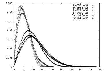
a                                                     b                                                     c

Figure 19: Mean shortest path length distribution $P(\ell)$ for several simulated PTNs. a: $\mathds{L}$-space; b: $\mathds{P}$-space; c: $\mathds{C}$-space. Symbols correspond to simulation results, curves to fits of unimodal distributions.

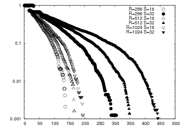
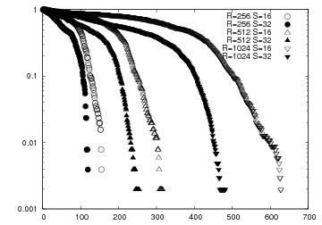
a                                                           b

Figure 20: Cumulative node degree distributions $P^{\rm cum}(k)$ (3) for several simulated PTNs in (a) $\mathds{P}$ and (b) $\mathds{C}$-spaces.

From the above qualitative investigation we conclude that realistic PTN maps are obtained for small or vanishing $a$ and $b\geq 0.5$. To quantitatively investigate the behavior of the simulated networks on their parameters including $R$ and $S$ let us now compare their statistical characteristics with those we have empirically obtained for the real-world networks. In Table 5 we have chosen to list the same characteristics of the simulated PTN as they are displayed for the real-world networks in Table 2. To provide for additional checks of the correlations between simulated and real-world networks, we present the characteristics in all $\mathds{L}$, $\mathds{P}$, and $\mathds{C}$-spaces. Let us note that our choice of the underlying grid to be a square lattice limits the number of nearest neighbors of a given station in $\mathds{L}$-space to $k_{\mathds{L}}\leq 4$. Moreover, as far as no direct links between these neighbors occur, the clustering coefficient in $\mathds{L}$-space vanishes, $c_{\mathds{L}}=0$. Nonetheless, as we discuss below, both characteristics display nontrivial behavior similar to real-world networks when displayed in $\mathds{P}$ and $\mathds{C}$-spaces.

For reasons explained above we choose a vanishing parameter $a=0$ and $b=0.5$ and for comparison $b=5.0$. The data shown in the Table was obtained for simulated PTNs of different numbers of routes, $R=256,\,512,\,1024$ and route lengths $L=16,\,32,\,64$. In the range of parameters covered in the Table we observe only weak changes of the various characteristics. Natural trends are that with the increase of the number of routes $R$ the maximal and mean shortest path length increases in all spaces. Most pronounced this is observed in $\mathds{L}$-space, while it is weakest in $\mathds{C}$-space. A similar increase is observed in $\mathds{L}$-space when increasing the number of stations $S$ per route. Choosing the values of $R$ in the range $R=256\div 1024$ and $S=16$, $S=32$ the average and maximal values of the characteristics studied here are found within the ranges seen for real-world PTNs, see Table 2. More detailed information is contained in the distributions of these characteristics and their correlations.

We restrict the further discussion to simulated PTNs described by $R=256,512,1024$, $S=16,32$, and $a=0$, $b=0.5$, which appear to reproduce many of the characteristics of real-world PTNs. In figure 19 we display the mean shortest path length distribution for these selected PTNs in $\mathds{L}$, $\mathds{P}$, and $\mathds{C}$-spaces. In $\mathds{L}$-space we observe two groups of distributions which correspond to the two route lengths $S=16$ and $S=32$. The most probable values for the path length $\hat{\ell}_{\mathds{L}}$ being of the order of the corresponding $S$. In $\mathds{P}$ and $\mathds{C}$-spaces the distributions are very similar with most probable path lengths $\hat{\ell}_{\mathds{P}}\sim 3$, $\hat{\ell}_{\mathds{C}}\sim 2$. In all cases the distributions are well fitted by the asymmetric unimodal distribution (12) and resemble those of the real-world networks shown in Fig. 7. Varying $b=0.2\div 5$ does not significantly change this picture.

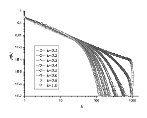
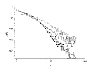
a                                                     b

Figure 21: a: Averaged (over $3000\div 30000$ simulated cities) station node degree distributions in $\mathds{B}$-space. $R=1024$, $S=64$, $a=0$. Parameter $b$ changes in the region $b=0.1\div 1.0$ as shown in the legend. b: Corresponding node degree distributions for Hamburg (circles), Hong Kong (squares), Los Angeles (triangles), and Istanbul (stars).

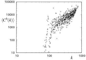
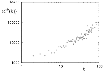
a                                                     b                                                     c

Figure 22: Mean betweenness centrality $\langle{\cal C}^{b}(k)\rangle$ for the simulated city of $300\times 300$ sites with $R=500$, $S=50$, $a=0$, and $b=0.5$ in $\mathds{C}$ (a), $\mathds{P}$ (b), and $\mathds{B}$ (c) spaces.

Let us now examine the node degree distributions of the simulated PTNs selected above. As explained above, the $\mathds{L}$-space degrees are restricted by the geometry of the underlying square lattice. Thus of the representations discussed here one may observe non-trivial distributions only in $\mathds{P}$, $\mathds{C}$, and $\mathds{B}$-spaces. Fig. 20a shows the cumulative node degree distribution in $\mathds{P}$-space in semi-logarithmic scale. Recall that for the majority of real-world PTNs studied in section III as well as in other works Sienkiewicz05 ; Xu07 , the $\mathds{P}$-space node degree distribution was found to decay exponentially. All distributions shown in Fig. 20a display two regions each governed by an exponential decay with a separate scale. Note that increasing both $S$ and $R$ leads to an increase of the ranges over which these regions extend. Comparing these results with those of Fig. 4b for real-world PTNs we find that all ranges observed there are also reproduced here. Within the parameter ranges chosen here the current model does not seem to attain a power law node degree distribution in $\mathds{P}$-space.

Comparing the$\mathds{C}$-space node degree distributions for real-world and simulated PTNs (Figs. 4c and 20b, correspondingly) one finds a definite tendency to an exponential behavior with two different scales in both cases. Note however that for the simulated PTNs the scales increase with the number of routes $R$ while they decrease with the number of stations per route $S$.

The simulated results discussed so far concerned data obtained for individual instances of modeled PTNs. One of the reasons for this was to reduce the computational effort required for the calculation of path lengths, betweennesses, and related global characteristics. Furthermore, in particular for the simulations involving high number of routes some self averaging may be expected to occur. The latter assumption was tested and verified by (i) simulating a reasonable set of PTNs with the same choice of parameters and (ii) by performing large-scale simulations calculating local characteristics. A result of the latter procedure involving averages over up to $3\cdot 10^{4}$ instances of simulated networks is shown in Fig. 21a. There we show the node degree distribution of the station nodes in $\mathds{B}$-space, i.e. the bipartite network of routes and stations with the inherent neighborhood relation (see Fig. 3). As can be seen in the double logarithmic plot shown in Fig. 21a a power-law like behavior of this distribution that extends over a wider range is found for small values of the parameter $b$. This corresponds to a situation where one finds many routes to proceed in parallel (compare with the maps shown in Fig. 18). For the more realistic choices of the $b$ parameter the overall behavior of this distribution is described by an exponential decay. The scale of this decay strongly depends on $b$. Fig. 21b shows that similar distributions for the real cities have oscillating character, which is caused by the fact that non-cumulative distributions are plotted. Similarly, individual distributions for simulated PTNs are in general non-monotonous, however the large number average of the distribution appears to be monotonously decreasing. Nevertheless, comparing plots in Figs. 21a and 21b one sees that in general the model is capable to reproduce the global decay properties of the station node degree distributions in $\mathds{B}$-space.

In Fig. 22 we show the betweenness-degree correlation for the simulated PTN with $X=300$, $R=500$, $S=50$, $a=0$, and $b=0.5$. There, we present the mean betweenness centrality $\langle{\cal C}^{b}(k)\rangle$ in $\mathds{C}$, $\mathds{P}$, and $\mathds{B}$-spaces. Corresponding plots for a real world network are shown in Fig. 14. Plots displayed for the simulated networks in Figs. 22a - 22c qualitatively reproduce the behavior of $\langle{\cal C}^{b}(k)\rangle$ observed for the real world networks in $\mathds{C}$, $\mathds{P}$, and $\mathds{B}$-spaces. $\mathds{L}$-space behavior can not be reproduced due to the restrictions caused by the geometry of the underlying square lattice.

In Figs. 23a and 23b we plot the cumulative harness distributions $P(r,s)$ for two simulated networks with $R=256$, $S=32$, $a=0$ and different values of parameter $b$: $b=0.2$ (Fig. 23a) and $b=1.0$ (Fig. 23b). Similar plots for real world networks are given in Figs. 16 and 17. The plots of Fig. 23 nicely reproduce two regimes empirically observed for the real-world PTN. In the first, the harness distribution is governed by a power law decay (25), Fig. 23a, whereas in the other one there is a tendency to an exponential decay (26), Fig. 23b. A prominent feature demonstrated by Fig. 23 is that one can tune the decay regime by changing the parameter $b$. For small values of $b$ the probability of a route to proceed in parallel with other routes is high c.f. Eq. (29). Therefore, the number of “hubs” in the $P(r,s)$ distribution of lines of several routes that go in parallel is large for small $b$. This is reflected by a power-law decay of the distribution. Alternatively, an increase of $b$ leads to a decrease of such hubs as shown by the exponential decay of their distribution.

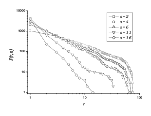
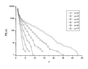
a                                                     b

Figure 23: Cumulative harness distributions $P(r,s)$ for the simulated PTN with $R=256$, $S=32$. Fig. a: $a=0$, $b=0.2$, fig. b: $a=0$, $b=1.0$. Compare with plots in Figs. 16, 17 for the real-world networks.

Summarizing the comparison of the statistical characteristics of real world networks with those of simulated ones one can definitely state that the model proposed above captures many essential features of real world PTNs. This is especially evident if one includes into the the comparison different network representations (different spaces) as performed above.

VII Conclusions

This paper was driven by two main objectives towards the analysis of urban public transport networks. First, we wanted to present a comprehensive survey of statistical properties of PTNs based on the data for cities of so far unexplored network size (see Table 1). Based on this survey, the second objective was to present a model that albeit being simple enough is capable to reproduce a majority of these properties.

Especially helpful in our analysis was the use of different network representations (different spaces, introduced in section II). Whereas former PTN studies used some of these representations, here within a comprehensive approach we calculate PTN characteristics as they show up in $\mathds{L}$, $\mathds{P}$, $\mathds{C}$, and $\mathds{B}$-spaces. It is the comparative analysis of empirical data in different spaces that enabled, in particular, an adequate PTN modeling presented in section VI.

The networks under consideration appear to be strongly correlated small-world structures with high values of clustering coefficients (especially in $\mathds{L}$ and less in $\mathds{C}$-spaces) and comparatively low mean shortest path values, as listed in Table 2. Standard network characteristics listed there correspond to the features a passenger is interested in when using public traffic in a given city. To give several examples, any two stops in Paris are on the average separated by $\langle\ell_{\mathds{L}}\rangle-1=5.4$ stations (with a maximal value of $\ell_{\mathds{L}}^{\rm max}-1=27$) and to travel between them one on average should do $\langle\ell_{\mathds{P}}\rangle-1=1.7$ changes. Evidence of correlations present in PTNs are the power-law node degree distributions observed for many networks in $\mathds{L}$ and for some in $\mathds{P}$-space (see Table 4). Currently, we find no explanation why some of the networks of our survey are governed by power-law node degree distributions whereas others follow an exponential decay. In the analysis of urban street networks a classification has been found Cardillo06 ; Volchenkov that allows to discriminate between properties of different classes of city organization. Let us note however that as a rule the latter analysis is performed for restricted regions of street networks i.e. either the historical or the suburban part. In the case of a PTN, however, one usually deals with a structure that spreads over all the city, covering both the inner and outer regions.

Besides looking on traditional network characteristics (as described in sections III - V) we addressed here a specific feature which is unique for PTNs and networks with similar construction principles. Namely, we analyzed statistical distributions of public transport routes that go in parallel for a sequence of stations. As we have shown such distributions (we call them harness distributions) are well defined for the networks under consideration and may be also be used for a quantitative description of similar networks embedded in 2D or 3D space as cables, pipes, neurons, or (blood-) vessels, etc.

The common statistical features of the networks considered emerge due to their common functional purposes and construction principles also reflected in the underlying bipartite structure Guillaume06 . It is this structure that explains parts of the correlations present in PTNs Seaton04 . The network growth model we present in Section VI captures this structure describing network evolution in terms of adding public transport routes, each of them being a complete graph in $\mathds{P}$-space. Our choice to use a self avoiding walk (SAW) as a route model in lattice simulations was motivated by geographical observations and other reasons, as argued in section VI. In support of the scaling argument given there, one may note that the fractal dimension of a SAW on a lattice does not change if a weak uncorrelated disorder is present, i.e. when some lattice sites can not be visited saw_disorder . In turn, this tells that the model is robust with respect to weak disturbances of the underlying lattice structure. Further analysis of simulated PTNs performed in section VI established strong similarities in the statistical characteristics of simulated and real-world networks.

Obviously, the two objectives in the PTN study we have so far achieved in this paper - the empirical analysis and the modeling - naturally call for an analytic approach. In particular, such approach may be used in parallel with numerical simulations to derive statistical properties of the model proposed in section VI. This will be a task for forthcoming studies. Another natural continuation of this work will be to analyze different possibly dynamic phenomena that may occur on and with PTNs. A particular task will be to study robustness of PTNs to targeted attacks and random failures Ferber07c .

Yu.H. acknowledges support of the Austrian FWF project 19583-PHY.

References

- (1) R. Albert and A.-L. Barabási, Rev. Mod. Phys. 74, 47 (2002).
- (2) S. N. Dorogovtsev and J. F. F. Mendes, Adv. Phys. 51, 1079 (2002).
- (3) M. E. J. Newman, SIAM Review 45, 167 (2003).
- (4) S. N. Dorogovtsev and S. N. Mendes, Evolution of Networks (Oxford University Press, Oxford, 2003).
- (5) Yu. Holovatch, O. Olemskoi, C. von Ferber, T. Holovatch, O. Mryglod, I. Olemskoi, and V. Palchykov, J.Phys. Stud. 10, 247 (2006).
- (6) L. A. N. Amaral, A. Scala, M. Barthélémy, and H. E. Stanley, Proc. Natl. Acad. Sci. USA., 97, 11149 (2000).
- (7) R. Guimera and L. A. N. Amaral, Eur. Phys. J. B 38, 381 (2004).
- (8) R. Guimera, S. Mossa, A. Turtschi, and L.A.N. Amaral, Proc. Nat. Acad. Sci. USA 102, 7794 (2005).
- (9) A. Barrat, M. Barthélemy, R. Pastor-Satorras, and A. Vespignani, Proc. Nat. Acad. Sci. USA 101, 3747 (2004).
- (10) L.-P. Chi, R. Wang, H. Su, X.-P. Xu, J.-S. Zhao, W. Li, and X. Cai, Chin. Phys. Lett. 20, 1393 (2003).
- (11) Y. He, X. Zhu, and D.-R. He, Int. J. Mod. Phys. B 18, 2595 (2004).
- (12) W. Li and X. Cai, Phys. Rev. E 69, 046106 (2004).
- (13) W. Li, Q. A. Wang, L. Nivanen, and A. Le Méhauté, Physica A 368, 262 (2006).
- (14) P. Sen, S. Dasgupta, A. Chatterjee, P. A. Sreeram, G. Mukherjee, and S. S. Manna, Phys. Rev. E 67, 036106 (2003).
- (15) P. Crucitti, V. Latora, and M. Marchiori, Physica A 338, 92 (2004).
- (16) R. Albert, I. Albert, and G. L. Nakarado, Phys. Rev. E 69, 025103 (2004).
- (17) M. Marchiori and V. Latora, Physica A 285, 539 (2000).
- (18) V. Latora and M. Marchiori, Phys. Rev. Lett. 87, 198701 (2001).
- (19) V. Latora and M. Marchiori, Physica A 314, 109 (2002).
- (20) K. A. Seaton and L. M. Hackett, Physica A 339, 635 (2004).
- (21) C. von Ferber, Yu. Holovatch, and V. Palchykov, Condens. Matter Phys. 8, 225 (2005), e-print cond-mat/0501296.
- (22) J. Sienkiewicz and J. A. Holyst, Phys. Rev. E 72, 046127 (2005), e-print physics/0506074; J. Sienkiewicz and J. A. Holyst, Acta Phys. Polonica B 36, 1771 (2005).
- (23) P. Angeloudis and D. Fisk, Physica A 367, 553 (2006).
- (24) P.-P. Zhang, K. Chen, Y. He, T. Zhou, B.-B. Su, Y. Jin, H. Chang, Y.-P. Zhou, L.-C. Sun, B.-H. Wang, and D.-R. He, Physica A 360, 599 (2006).
- (25) C. von Ferber, T. Holovatch, Yu. Holovatch, and V. Palchykov, Physica A 380, 585 (2007).
- (26) H. Chang, B.-B. Su, Y.-P. Zhou, and D.-R. He, Physica A 383, 687 (2007).
- (27) X. Xu, J. Hu, F. Liu, and L. Liu, Physica A 374, 441 (2007).
- (28) C. von Ferber, T. Holovatch, Yu. Holovatch, and V. Palchykov, arXiv:0709.3203. In Traffic and Granular Flow ’07. Springer (2008) (to appear).
- (29) C. von Ferber, T. Holovatch, and Yu. Holovatch, arXiv:0709.3206. In Traffic and Granular Flow ’07. Springer (2008) (to appear)
- (30) For links see http://www.apta.com.
- (31) Some numbers for the real-world PTNs slightly differ from those from our letter Ferber07a . The reason is an improvement of the database.
- (32) H. A. Simon, Biometrica 42, 425 (1955).
- (33) D. de S. Price, J. Amer. Soc. Inform. Sci. 27, 292 (1976).
- (34) A.-L. Barabási and R. Albert, Science 286, 509 (1999); A.-L. Barabási, R. Albert, and H. Jeong, Physica A 272, 173 (1999).
- (35) R. Ferrer i Cancho and R. V. Solé, e-print cond-mat/0111222; S. Valverde, R. Ferrer i Cancho, and R. V. Solé, Europhys. Lett. 60, 512 (2002); R. Ferrer i Cancho and R. V. Solé, in Statistical mechanics of Complex Networks, edited by R. Pastor-Satorras, M. Rubi, and A. Diaz-Guilera (Lecture Notes in Physics Vol 625, Springer, Berlin, 2003), p. 114.
- (36) M. T. Gastner and M. E. J. Newman, Eur. Phys. J. B 49, 247 (2006).
- (37) N. Mathias and V. Gopal, Phys. Rev. E 63, 021117 (2001).
- (38) R. Ferrer i Cancho and R. V. Solé, Proc. Natl. Acad. Sci. USA., 100, 788 (2003); R. Ferrer i Cancho, Physica A, 345, 275 (2005).
- (39) A. Cardillo, S. Scellato, V. Latora, and S. Porta, Phys. Rev. E 73, 066107 (2006).
- (40) P. Erdös and A. Rényi, Publ. Math. (Debrecen) 6, 290 (1959); Publ. Math. Inst. Hung. Acad. Sci. 5, 17 (1960); Bull. Inst. Int. Stat. 38, 343 (1961).
- (41) B. Bollobás, Random Graphs (Academic Press, London, 1985).
- (42) J. A. Holyst, J. Sienkiewicz, A. Fronczak, P. Fronczak, and K. Suchecki, Phys. Rev. E 72, 026108 (2005).
- (43) A. Fronczak, P. Fronczak, and J. A. Holyst, Phys. Rev. E 68, 046126 (2003).
- (44) U. Brandes, J. Math. Sociology 25, 163 (2001).
- (45) G. Sabidussi, Psychometrika 31, 581 (1966).
- (46) P. Hage and F. Harary, Social Networks 17, 57 (1995).
- (47) A. Shimbel, Bull. Math. Biophys. 15, 501 (1953).
- (48) L. C. Freeman, Sociometry 40, 35 (1977).
- (49) K.-I. Goh, B. Kahng, and D. Kim, Phys. Rev. Lett. 87, 278701 (2001).
- (50) M. E. J. Newman, Phys. Rev. Lett. 89, 208701 (2002).
- (51) M. E. J. Newman, Phys. Rev. E 67, 026126 (2003).
- (52) M. E. J. Newman, S. H. Strogatz, and D. J. Watts, Phys. Rev. E 64, 026118 (2001).
- (53) Z. Liu, Y.-C. Lai, N. Ye, and P. Dasgupta, Phys. Lett. A 303, 337 (2002).
- (54) M.E.J. Newman, Phys. Rev. E 64, 016131 (2001).
- (55) X. Li and G. Chen, Physica A 328, 274 (2003).
- (56) J.J. Ramasco, S.N. Dorogovtsev, and R. Pastor-Satorras, Phys. Rev. E 70, 036106 (2004).
- (57) J.-L. Guillaume and M. Latapy, Physica A 371, 795 (2006).
- (58) B. Nienhuis, Phys. Rev. Lett. 49, 1062 (1982).
- (59) D. Volchenkov and Ph. Blanchard, Phys. Rev. E 75, 026104 (2007); D. Volchenkov, Condens. Matter Phys. (2008), to appear.
- (60) A.B. Harris, Z. Phys. B 49, 347 (1983); Y. Kim, J. Phys. C 16, 1345 (1983); V. Blavats’ka, C. von Ferber, and Yu. Holovatch, Phys. Rev. E, 64, 041102 (2001); C. von Ferber, V. Blavats’ka, R. Folk, and Yu. Holovatch, Phys. Rev. E 70, 035104(R) (2004).