LOCALIZED — DELOCALIZED ELECTRON QUANTUM PHASE TRANSITIONS

Abstract

Metal–insulator transitions and transitions between different quantum Hall liquids are used to describe the physical ideas forming the basis of quantum phase transitions and the methods of application of theoretical results in processing experimental data. The following two theoretical schemes are discussed and compared: the general theory of quantum phase transitions, which has been developed according to the theory of thermodynamic phase transitions and relies on the concept of a partition function, and a theory which is based on a scaling hypothesis and the renormalization-group concept borrowed from quantum electrodynamics, with the results formulated in terms of flow diagrams.

CONTENT

1. Introduction

1.1. Thermal and quantum fluctuations.
2. Quantum phase transitions

2.1. Definition of a quantum phase transition . 2.2. Parallels and differences between classical and quantum phase transitions 2.3. Critical region of a quantum phase transition.
3. Flow diagrams for metal–insulator transitions
4. Three-dimensional electron gas
5. Two-dimensional electron gas

5.1. Gas of noninteracting electrons 5.2. Spin–orbit interaction 5.3. Gas of interacting electrons.
6. Quantum transitions between the different states of a Hall liquid
7. Conclusion

I 1. Introduction

Quantum phase transitions that occur in an electron gas and result in localization represent the mainstream in the study of electrons in solids; it is directed toward low temperatures and interactions. We think that a dangerous gap between theory and experiment has appeared in this field of science. The related theories are so complex that experimentalists, as rule, use ready recipes and formulas of these theories without knowing (and, hence, without controlling) all the initial assumptions and limitations.

In this review, we will try to close this gap. Our review does not contain a sequential description of the mathematical techniques involved in formulating hypotheses and theories. Instead, we outline the physical ideas, concepts, and assumptions that are often omitted in theoretical works and reviews, especially at the stage of a developed theory. This specific feature is thought to make our review interesting and useful for experimentalists.

On the other hand, we did not tend to accumulate, classify, and estimate the huge experimental data obtained in this field. We address experiment to demonstrate the use of a theory for its interpretation and the related difficulties and problems. This specific feature is thought to make our review interesting and useful for theorists.

We first qualitatively discuss the ides that constitute the basis of the theory of quantum phase transitions. We then consider how the general theoretical scheme can describe the well-known data on metal–insulator transitions and transitions between different quantum Hall liquids.

1.1. Thermal and quantum fluctuations

Before discussing quantum phase transitions in essence, we briefly recall some facts from statistical physics. We consider a macroscopic system consisting of a huge number of particles. This system is almost isolated and behaves mainly as a closed system; however, it can exchange particles and energy with a larger system, which serves as a reservoir. In other words, our system is a subsystem of this reservoir.

We first analyze the classical subsystem at a finite temperature T. According to classical statistics formulas, the probability $p_{i}$ for the subsystem to occupy the state with energy $\varepsilon_{i}$ is

$$p_{i}=\frac{e^{-\varepsilon_{i}/T}}{Z}\>,$$ (1)

where the coefficient $1/Z$ is determined by the normalization condition $\sum p_{i}=1$

$$Z=\sum_{i}\exp(-\varepsilon_{i}/T)$$ (2)

(hereafter, temperature is given in energy units). Function $Z$ is called the partition function. It plays a key role in the description of the thermodynamic properties of classical objects. That the subsystem energy obeys distribution (1) rather than being fixed means the presence of classical thermal fluctuations.

When quantum mechanics appeared, the basis of classical thermodynamics and its principal formulas were revised. The classical expressions were found to have a limited field of application. Quantum statistics requires a developed quantum-mechanics math-based environment. Before addressing this environment, we assume that the subsystem is completely closed and does not interact with the large system. As a result, we can use the standard quantum mechanics technique and use the Schrödinger steady-state equation to describe the subsystem. The resulting set of steady-state energies $\varepsilon_{i}$ and the corresponding wavefunctions $\varphi_{i}(q)$ of the subsystem are considered to be subsystem attributes in the zeroth approximation. These energies, $\varepsilon_{i}$, enter Eqn (2). The set of $\varphi_{i}(q)$ functions is convenient because it is related to the subsystem under study and is a complete set; therefore, it can be used for expansion into a series.

The presence of a huge number of particles in the subsystem implies that it has a very dense energy distribution of quantum levels. Due to a weak interaction with the reservoir, the subsystem is in the so-called mixed state, in which no measurement or a set of measurements can lead to unambiguously predicted results. Upon determining the mixed state, the repeated measurements of any physical quantity give a near-average result that differs from the previous one. The scatter of the measured physical quantities is interpreted as a result of fluctuations.

Because the subsystem interacts with the environment, it cannot be described by a wave function; therefore, the wave function is substituted by a density matrix,

$$\rho(q^{\prime},q)=\int\psi^{*}(q^{\prime},X)\psi(q,X)dX,$$ (3)

where $q$ corresponds to the set of subsystem coordinates, $X$ are the remaining coordinates of the system, and $\psi(q,X\,)$ is the wave function of the closed system.

The mean values of any physical quantity $\langle s\rangle$ are now calculated using the density matrix

$$\langle s\rangle=\frac{1}{A}\int\left\{\widehat{s}[\rho(q^{\prime},q)]\rule[-5.69054pt]{0.0pt}{12.0pt}\right\}_{q^{\prime}=q}dq,\qquad A=\int\rho(q,q)dq.$$ (4)

rather than a wave function. In Eqn (4), we apply the operator $\widehat{s}$, which acts on functions of the variable $q$, to the density matrix $\rho(q\,^{\prime},q)$; we then set $q\,^{\prime}=q$ and integrate. The operator that formally enters the expression for the normalization factor $A$ is identical with unity; therefore, the condition $q\,^{\prime}=q$ is naturally taken into account in the integrand.

According to general rule(4), the mean of coordinate $\langle q\rangle$, for example, is given by

$$\langle q\rangle=\frac{1}{A}\int\int\psi^{*}(q,X)q\psi(q,X)dqdX=\frac{\int q\rho(q,q)dq}{\int\rho(q,q)dq}.$$ (5)

The physical meaning of the density matrix can be clarified if we write it in an explicit form for the subsystem in statistical equilibrium at a finite temperature $T$:

$$\rho(q^{\prime},q)=\sum_{i}\varphi_{i}^{*}(q^{\prime})\varphi_{i}(q)e^{-\varepsilon_{i}/T}.$$ (6)

For the subsystem in statistical equilibrium, it follows from Eqns (5) and (6)

$$\langle q\rangle=\frac{1}{A}\sum_{i}\int\varphi_{i}^{*}(q)\varphi_{i}(q)e^{-\varepsilon_{i}/T}qdq=\frac{1}{A}\sum_{i}\langle q\rangle_{i}e^{-\varepsilon_{i}/T},\qquad{\langle q\rangle}_{i}=\int\varphi_{i}^{*}(q)\varphi_{i}(q)qdq.$$ (7)

The averaging with the density matrix performed in Eqn (7) account for both the probabilistic description in the form of $\langle q\rangle_{i}$ in quantum mechanics and incomplete information about the system (statistical averaging).

We use the $\varphi_{i}(q)$ functions and write the function $\rho(q\,^{\prime},q)$ in the matrix form

$$\rho(q^{\prime},q)=\|\rho_{ij}\|=\left\|\int\varphi_{j}^{*}(q)\rho(q^{\prime},q)\varphi_{i}(q)dq\right\|.$$ (8)

In Eqn (4), we then have

$$\langle s\rangle=\frac{\sum_{ij}s_{ij}\rho_{ji}}{\sum_{i}\rho_{ii}}=\sum_{ij}s_{ij}w_{ji},\qquad w_{ij}=\frac{\rho_{ij}}{\sum_{i}\rho_{ii}}.$$ (9)

The $w_{i\,j}$ matrix constructed from the set of $\varphi_{i}(q)$ functions is called the statistical matrix and, in essence, is the normalized density matrix.

We replace $\widehat{s}$ with the energy operator $\widehat{H}$ in Eqn (4) and obtain

$$\langle\varepsilon\rangle=\sum_{i}w_{ii}\varepsilon_{i}.$$ (10)

This means that the probability $p_{i}$ of detecting the energy $\varepsilon_{i}$ in the subsystem is equal to the diagonal element of the matrix $w_{ii}$,

$$p_{i}={w}_{ii}.$$ (11)

Equation (11) is the quantum analog of Eqn (1).

The statistical matrix has a number of universal properties. By definition, this matrix is normalized:

$$\sum_{i}w_{ii}=1.$$ (12)

As follows from Eqn (6), the statistical matrix is diagonal in statistical equilibrium. Its diagonal elements are functions of only the energy of the corresponding subsystem state $\varepsilon_{i}$. Until at least one $w_{ii}$ with $i\neq 0$ has a nonzero value, the subsystem state remains mixed, and any measured quantity undergoes fluctuations.

The macroscopic system is in a mixed state mainly due to a finite temperature. A comparison of Eqns (1) and (11) demonstrates that in the high-temperature limit, the statistical matrix obeys the Gibbs distribution

$$w_{ii}=\exp(-\varepsilon_{i}/T)/Z.$$ (13)

with a good accuracy.

Because the integral of the squared wave function $\varphi_{i}(q)$ over the entire coordinate space is

$$\int\varphi_{i}^{*}(q)\varphi_{i}(q)dq\equiv 1,$$

the partition function $Z$ can be represented as the sum of the diagonal matrix elements of the operator $\exp{(-\widehat{H}/T\,)}$ over the complete set of eigenfunctions $\varphi_{i}$:

$$Z=\sum\limits_{i}\int\varphi_{i}^{*}(q)\varphi_{i}(q)e^{-\varepsilon_{i}/T}dq=\sum_{i}\langle\varphi_{i}|\exp(-\widehat{H}/T)|\varphi_{i}\rangle.$$ (14)

Here, we use that $\varphi_{i}$ are eigenfunctions of the Hamiltonian $\widehat{H}$ to obtain

$$\exp(-\widehat{H}/T)\varphi_{i}=e^{-\varepsilon_{i}/T}\varphi_{i}$$

.

A comparison of Eqns (4)—(7) with Eqn (13) gives another form of the partition function,

$$Z=\int\rho(q,q)dq\equiv\mbox{Sp}[\rho(q^{\prime},q)].$$ (15)

If $Z$ is regarded as a normalization factor, Eqns (4) and (9) demonstrate that representation (15) is valid in both the classical limit and general case.

As the subsystem is open, it interacts with the environment. Even if this interaction is very weak, the states of the macroscopic system become mixed in a certain small energy range due to the extremely high density of the system energy levels. Therefore, even at zero temperature, the unclosed subsystem is in a mixed state. This means that as the temperature decreases, each $w_{ii}\,$ $(i\neq 0)$ element approaches a temperature-independent constant, which depends on $\varepsilon_{i}$ and the sizes and properties of the subsystem, rather than tending to zero exponentially. Thermal fluctuations are replaced by quantum fluctuations. This statement is illustrated by Fig. 1a, which qualitatively shows the temperature dependence of the probability $p_{i}$ of detecting the energy $\varepsilon_{i}$ in the subsystem. The dashed lines separate the regions of predominantly quantum and predominantly thermal fluctuations. The limiting value $p_{i}(0)$ is specified by the energy $\varepsilon_{i}$, sizes, and properties of the subsystem.

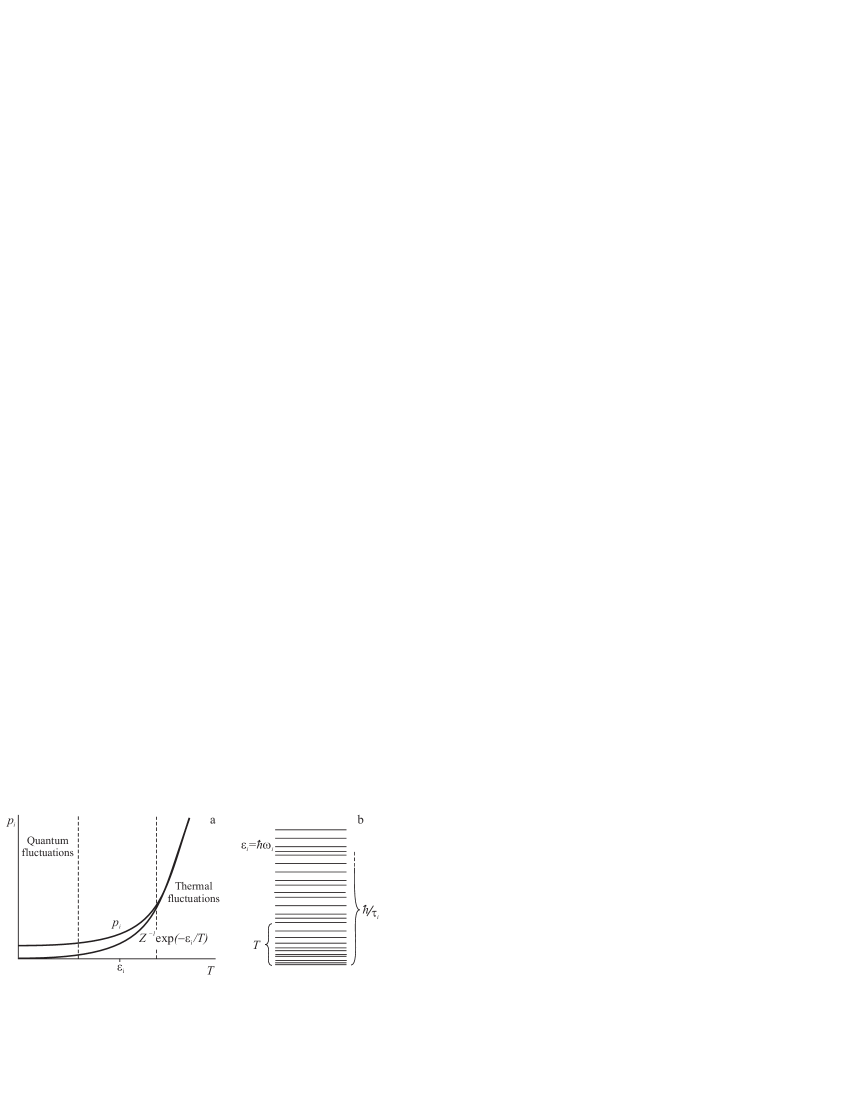
Figure 1: (a) Low-temperature behavior of the diagonal elements $w_{ii}$ of the statistical matrix corresponding to low energies. (b) Simultaneous excitation of thermal and quantum fluctuations

In this subsystem, $p_{i}(0)$ obviously decreases with an increase in $\varepsilon_{i}$. We assume that this dependence is a power-law function, $p_{i}(0)\propto 1/\varepsilon_{i}^{\,\alpha}$, and obtain the lower estimate of the exponent $\alpha$. Energy for thermal fluctuations is taken from the reservoir. A finite, not exponentially small, probability of detecting the subsystem in a state $\varepsilon_{i}\gg T$ means a violation of the energy conservation law. This violation can exist in the framework determined by the uncertainty relation

$$\varepsilon_{i}\tau_{i}\sim\hbar,$$ (16)

where $\tau_{i}$ is the lifetime of the state $\varepsilon_{i}$. Therefore, even if transitions to all $\varepsilon_{i}$ states were equiprobable, $p_{i}(0)$ would decrease according to the law $p_{i}(0)\propto\varepsilon_{i}^{\,-1}$, as follows from Eqn (16) . As a result, we have

$$\alpha\geqslant 1.$$ (17)

It is essential that the energy range in which quantum fluctuations occur is temperature independent, which follows from uncertainty relation (16).

The relative role of thermal and quantum fluctuations is illustrated in Fig. 1b, which shows the excitation spectrum of the subsystem in one of the phases, i.e., far from phase transition point $x=x_{\rm c}$. The brace in the bottom left part of Fig. 1b indicates the temperature-related scale. Only modes with frequencies $\omega_{i}\,\lesssim\,T/\hbar$ are classically excited modes. Although the range of thermal modes is bounded above by temperature, they have large occupation numbers. Modes with $\omega_{i}>T/\hbar$ are mainly excited due to quantum processes and have small occupation numbers. However, as the temperature decreases, the role of quantum excitations increases.

II 2. Quantum phase transitions

2.1 Definition of a quantum phase transition.

Quantum phase transitions are phase transitions that can occur at the absolute zero $T=0$ and consist of a change in the ground state of a system in the case where a certain control parameter $x$ takes a critical value $x_{\rm c}$. (The ground state is taken to be the lowest possible mixed state.) The control parameter can be, for instance, a magnetic field or an electron concentration. Quantum phase transitions belong to the class of continuous transitions at which none of the physical functions of state has a discontinuity at the transition point.

A quantum fluctuation is the only cause that can change the ground state of the system at zero temperature; the phase transitions under study are therefore called quantum phase transitions. As in the case of thermodynamic transitions, the concept of a correlation length $\xi$, which has the meaning of the average quantum-fluctuation size, is introduced into the theory of quantum phase transitions. At the absolute zero temperature, $\xi$ is only determined by the deviation $\delta x$ of the control parameter from the critical value. The dependence of $\xi$ on $\delta x$ is assumed to be a power-law function,

$$\xi\propto|x-x_{c}|^{-\nu}.$$ (18)

Real experiments are always performed at finite temperatures, where thermal fluctuations exist in addition to quantum fluctuations. The goal of the theory is to predict the manifestation of the phase transition that occurs only at zero temperature in the properties of the system at a finite temperature.

The theory of quantum phase transitions (see, e.g., book Sachdev or reviews QuantRev ; Vojta ) is analogous to the theory of thermodynamic phase transitions. In the $(x,T))$ plane (i.e., in a plane where temperature is plotted versus a control parameter), the quantum transition point can be a finite point on the line of thermodynamic transitions, $x_{\rm c}(T\,)\rightarrow x_{\rm c}(0)$ as $T\rightarrow 0$. For example, this behavior is characteristic of magnetic transitions with the magnetic field used as a control parameter. Quantum phase transitions of another type also exist; they are imaged by isolated point $x_{\rm c}$ on the abscissa axis of the $(x,T)$ plane. The metal–insulator transition is an example of such a transition. In this review, we restrict ourselves to the case of isolated-point transitions.

2.2 Parallels and differences between classical and quantum phase transitions

As noted above, quantum phase transitions belong to the class of continuous transitions; there are no two coexisting competitive phases and, hence, no stationary boundary between them. This class also includes thermodynamic second-order phase transitions. At a thermodynamic phase transition point, the system transforms into another phase as a whole as a result of thermal fluctuations. Fluctuations exist on either side of the transition, and their characteristic size $\xi$ is called the correlation length. As the transition is approached from either side, $\xi$ diverges PP ; Goldenfeld .

It is natural to expect a similar situation to occur in the vicinity of a quantum transition with the participation of quantum fluctuations. An analogy between classical and quantum phase transitions does exist, and it is rather unexpected. The behavior of a quantum system in the vicinity of a transition point at a finite temperature in a d-dimensional space is analogous to the behavior of a classical system in a space with dimension ${\cal D}>d$. This statement requires extensive explanations, which should include an algorithm for the introduction of such an imaginary system and the determination of its dimension.

First, we have to clearly distinguish between the dimension of the geometric space in which the system is located and the dimension of the generalized-coordinate space, which depends on the number of particles $\cal N$ in the system. If $\varrho$ is the density of particles in the space, we have ${\cal N}=\int\int\int\varrho d\,^{d}X$, where the dimension $d$ determines the multiplicity of the integral. Usually, a $d$-dimensional space is assumed to be infinite in all directions, but the range of one or several $X_{i}$ coordinates can be limited.

Second, we note a similarity between the operator $\exp{(-\widehat{H}/T\,)}$, which was used to write Eqn (14), and the operator $\widehat{S}$ that describes the evolution of a closed quantum system with time according to the Schrödinger equation

$${\rm i}\hbar\frac{\partial\psi}{\partial t}=\widehat{H}\psi,\qquad\widehat{S}=\exp(-\frac{{\rm i}}{\hbar}\widehat{H}t).$$ (19)

This similarity becomes obvious if we change the variables as

$${\rm i}t/\hbar=1/T.$$ (20)

With substitution (20), we can interpret the matrix elements in Eqn (14) differently. The element $\bigl{\langle}i\,\bigl{|}\,\exp{(-\widehat{H}/T\,)}\bigr{|}i\,\bigr{\rangle}$ can be regarded as the amplitude of the probability that, starting from state $\langle i\,|$, the subsystem evolves under the action of $\widehat{S}$ and returns to the initial state $|i\,\rangle$ within imaginary time $\tilde{t}$, which is equal to $-{\rm i}\hbar/T$. The imaginary time $\tilde{t}$ is often called the Matsubara time. For definiteness, we assume that the number of steps is fixed and equal to $N+1$, $N\gg 1$ and that, in time ${\rm i}\hbar/T$, the subsystem has passed through $N$ virtual states and occupied each state for a time $(\delta\tilde{t}\,)_{j}$; as a result, we have

$$\sum_{j=0}^{N}(\delta\tilde{t}\,)_{j}={\rm i}\hbar/T.$$ (21)

The amplitude of ‘the probability of returning to the initial state’ means the sum of the amplitudes of the probabilities of returning for all possible trajectories in the space of states. We consider a set of trajectories consisting of $N$ steps. The operator entering each matrix element in Eqn (14) is represented as

$$\exp(-\widehat{H}/kT)=\exp\left(\frac{{\rm i}}{\hbar}\widehat{H}\sum_{0}^{N}(\delta\tilde{t}\,)_{j}\right).$$ (22)

We take a complete set of wavefunctions $|m_{j}\rangle$ of an arbitrary operator that does not commute with the Hamiltonian and assume that the trajectories are realized in these states. Then, instead of Eqn (14), we obtain

$$Z=\sum\limits_{i}\sum\limits_{m_{1},m_{2},...m_{N}}<i|\exp(-{\rm i}\widehat{H}(\delta\tilde{t}\,)_{1}/\hbar)|m_{1}><m_{1}|\exp(-{\rm i}\widehat{H}(\delta\tilde{t}\,)_{2}/\hbar)|m_{2}>...<m_{N}|\exp(-{\rm i}\widehat{H}(\delta\tilde{t}\,)_{N}/\hbar)|i>.$$ (23)

The product of the matrix elements in the summand corresponds to a chain of consecutive virtual transitions. The summation over all $\{m_{j}\}$ combinations means that all possible closed chains of $N$ links are taken into account. The modification of the expression for $Z$ — the replacement of Eqn (14) with Eqn (23) — means that we take the quantum properties of the system into account by adding virtual transitions to real ones.

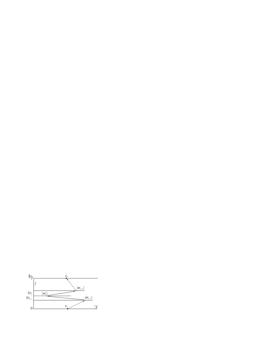
Figure 2: Set of quantum statistical $d$-dimensional systems located in a one-dimensional band of width $\hbar/T$and virtual transition between them

The introduction of virtual transitions is illustrated in Fig. 2, where the abscissa axis stands for the initial $d$-dimensional space $\{^{d}X\}$ and all possible classical states of the system are located along this axis in the order of increasing energy. All other horizontal lines are replicas of this space. These replicas form a set of $N$ elements in the segment $[0,\hbar/T\,]$. The black dot on the abscissa axis represents the initial state of the system with energy $\varepsilon_{i}$. The second black dot on the upper horizontal line corresponds to the ‘final’ state of the system with the same energy $\varepsilon_{i}$ at the maximum value of the imaginary time $|\tilde{t}\,|=\hbar/T$. The arrows indicate the chain of virtual transitions through the set of virtual states $|m_{j}\rangle$ designated by white dots. These are mixed states without a definite energy; therefore, they are not eigenstates of the operator $\widehat{H}$. The virtual transitions reflecting the quantum properties of the statistical system under study are shown by arrows. The chain of virtual transitions shown in Fig. 2 corresponds to one term in the sum in (23). The summation over all $\{m_{j}\}$ combinations means that we account for all possible chains between the fixed initial and final $\varepsilon_{i}$ points.

Now, the problem is to construct a classical system whose partition function is represented by Eqn (23). In the original Eqn (14), the summation over $i$ meant the summation over all the states realized in a $d$-dimensional system. The number of terms in the sum is now increased, and our real system does not have such a large number of different states. Nevertheless, we can construct an imaginary classical system with a higher dimension using the scheme shown in Fig. 2.

We add an additional axis for an imaginary time to the $d$ axes of the original space. In the graphical terms of Fig. 2, this means that an ordinate axis is added to the abscissa axis. It is seen from Eqn (21) that the coordinate along this new axis changes in the range

$$0\leqslant|\widetilde{t}|\leqslant\hbar/kT.$$ (24)

Each point in the strip (24) in Fig. 2 corresponds to some virtual state of the quantum system; it can be named the image point. The width (24) of strip in which an image point is located increases with decreasing the temperature. At $T=0$, the strip transforms into a half-plane; an increase in the temperature, in contrast, narrows the band and decreases its contribution to the statistical properties of the quantum system.

We repeat the $d$-dimensional classical system $N$ times by placing replicas along the imaginary time $\tilde{t}$ axis at a distance $(\delta\tilde{t})_{j}$ from each other. The states of the replicas in this ensemble can be different. Let these states be $m_{j}$. We fix a certain ‘initial’ state of the ‘lower’ subsystem $\varepsilon_{i}$. The energy of the classical ${\cal D}$-dimensional system, we are constructing, is equal to the sum of the energies of all layers, with allowance for the interaction between them. Each $\varepsilon_{i,\{m\}}$ corresponds to a certain energy $\varepsilon_{i}$ of the initial $d$-dimensional classical system and a certain chain of states entering Eqn (23). Therefore, the number of terms in the sum $\sum_{\{m\}}s_{i,\,m}$ in Eqn (23) is equal to the number of different $\varepsilon_{i,\{m\}}$ energies. We note that each $s_{i,\,m}$ term in sum has a form typical for partition sums, since the product of the matrix elements in this term eventually reduces to the product of $\exp{\bigl{(}-{\rm i}\varepsilon_{j}(\delta\tilde{t}\,)_{j}/\hbar\bigr{)}}$. The only difference is that for the classical system, each term in $Z$ is a real positive number and, in Eqn (23), a real positive number is represented by the sum $s_{i}=\sum_{\{m\}}s_{i,\,m}$ over $\{m\}$ of all $s_{i,\,m}$ products. When neglecting this difference, we can consider Eqn (23) the partition function $Z$ of the imaginary ${\cal D}$-dimensional classical system.

Of course, in the general form, the resulting mathematical construction is absolutely unpractical. However, as is customary in deriving scaling relations, it is important to reveal some significant properties of sum (23) rather than to calculate it. As is shown in Section 2.3, one of these properties is anisotropy, i.e., non equivalence of the axes of the ${\cal D}$-dimensional space.

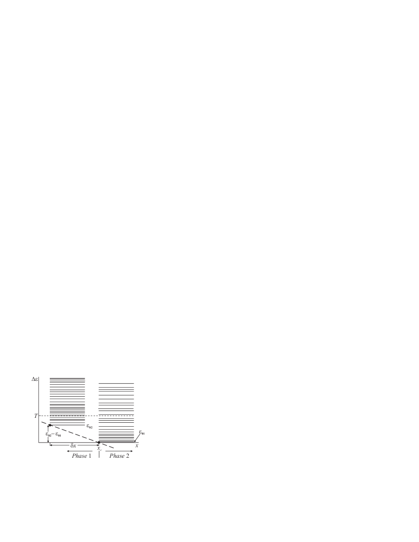
Figure 3: The difference in the lowest energies of two phases $\Delta\varepsilon=\varepsilon_{02}-\varepsilon_{01}$ versus a control parameter (dashed line). At a control parameter $x=x_{c}-\delta x$, phase 1 is subjected to fluctuation excitation inside equilibrium phase 2. Because $|\Delta\varepsilon|<T$, thermal fluctuation play a key role in this excitation

At a thermodynamic phase transition point, the partition function $Z$ has special features. The sensitivity of function (14) to the presence of a phase transition is caused by the fact that, when the transition is approached, the energy range $T$ determining significant terms in sum (14) contains not only $\varphi_{i}$ levels from the set corresponding to the equilibrium phase but also $\varphi_{i}^{\prime}$ levels from the nonequilibrium phase (Fig. 3). This allows fluctuation transitions between $|i\,\rangle$ and $|i\,^{\prime}\rangle$ levels from different sets. Additional possibilities appear after Eqn (14) is replaced with Eqn(23). If the temperature is low $(|\Delta\varepsilon|>T\,)$, the fluctuation-induced appearance of another phase is also possible, but due to quantum fluctuations.

2.3. Critical region of a quantum phase transition

A region in which all physical quantities depend only on the correlation length $\xi$ always exists in the phase plane near a classical phase transition. It is called the critical or scaling region. Near a quantum phase transition at $T=0$, there also exists a control parameter $\delta x$ range in which physical quantities are expressed through the length $\xi$ determined by Eqn (18). In Section 4, we show this behavior by the example of a metal–insulator transition in a three-dimensional system of noninteracting electrons, and determine the boundaries of this region. At a finite temperature $T\neq 0$, however, the scaling region of a quantum phase transition is more complex.

The space $\{^{d}X,\tilde{t}\,\}$ has dimension $d+1$ because of the additional imaginary time axis. We introduce correlation lengths in the space $\{^{d}X,\tilde{t}\,\}$. We retain the traditional notation $\xi$ for the correlation length in an ordinary $d$-dimensional subspace and let $\xi_{\varphi}$ denote the correlation length along the additional axis. The subscript $\varphi$ is a reminder that $\xi_{\varphi}$ is related to the quantum aspect of the problem and to the specific features of wave functions. The dimension of $\xi_{\varphi}$ is $\hbar/T$ rather than length; that is, it is measured in seconds rather than centimeters.

As $x\rightarrow x_{\rm c}$ and $T\rightarrow 0$, both correlation lengths diverge at a transition. According to the theory of continuous thermodynamic transitions, the divergence is described by power functions; but the exponents of the two correlation lengths can be different in general. This is usually written as

$$\xi\propto\delta x^{-\nu},\qquad\delta x=|x-x_{c}|,$$ (25)

$$\xi_{\varphi}\propto\xi^{z}.$$ (26)

The exponents $\nu$ and $z$ are called critical indices; $z$ is called the dynamic critical index. Both names and designations originate from the theory of thermodynamic processes. In particular, the dynamic critical index in the theory of thermodynamic processes enters the relation between the lifetime and size of thermal fluctuations, $\tau\propto\xi^{\,z}$. In the quantum problem at $T=0$, the situation is similar: the length $\xi$ characterizes spatial correlations, i.e., the characteristic size of quantum fluctuations, and the time $\xi_{\varphi}$ characterizes time correlations.

Formula (26) immediately fixes the dimension of the space in which the imaginary classical system should be placed. A real length must be the coordinate along all axes of this space; that is, length axes should be made from the $\tilde{t}$ axis. As follows from dimensional considerations and Eqn (26), the length equivalent to the ‘correlation pseudolength’ $\xi_{\varphi}$ is proportional to $\xi_{\varphi}^{1/z}$,

$$\zeta\propto\xi_{\varphi}^{1/z}.$$ (27)

Therefore, the volume element in the space is

$$(d\xi)^{d}d\xi_{\varphi}\propto(d\xi)^{d}(d\zeta)^{z}$$ (28)

and a $z$-dimensional subspace with the conventional ‘spatial’ coordinates appears instead of the one-dimensional imaginary time axis. Hence, we have

$${\cal D}=d+z.$$ (29)

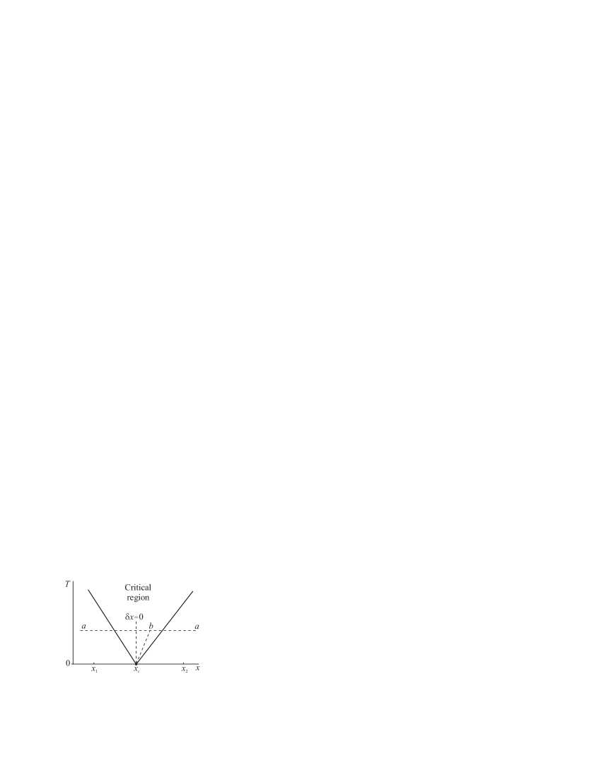
Figure 4: Shape of the critical region of a quantum phase transition depicted by an isolated point in the ($x,T$) plane

It is convenient to discuss the consequences of Eqns (25) and (26) using the $(x,T\,)$ plane (Fig. 4). At $T=0$, the control parameter $x$ on the abscissa axis of the $(x,T\,)$ plane only affects one independent correlation length, $\xi$, and $\xi_{\varphi}$ (and the length $\zeta$) can be formally obtained from $\xi$ using Eqn (26). All the physical quantities can be expressed only in terms of $x_{\rm c}$ in a certain segment $[x_{1},x_{2}]$ that contains the point $x_{\rm c}$.

Now, let the temperature $T\neq 0$. We move in the $(x,T\,)$ plane along a horizontal line $T\neq 0$ (Fig. 4, line $aa$) in the $x\rightarrow x_{\rm c}$ direction. At a certain value of $\delta x$, the length $\xi_{\varphi}$, which changes according to Eqns (25) and (26), reaches its maximum value $\hbar/T$ [which is determined by inequality (24)]. At lower values of $\delta x$, Eqn (26) does not hold on line $aa$, because $\xi$ increases according to Eqn (25) and $\xi_{\varphi}$ remains equal to its maximum value $\hbar/T$. The parameters $\xi$ and $\xi_{\varphi}$ become mutually independent. The region of this independence is called the critical region. If we now move toward the transition inside the critical region (e.g., along line $bx_{\rm c})$, both parameters still diverge at the transition. However, the divergence of one of them is controlled by $\delta x$, $\xi\propto\delta x^{\,-\nu}$, and the divergence of the other is controlled by temperature, $\xi_{\varphi}=\hbar/T$.

The name of the region derives from the fact that, for a quantum transition, the critical region is considered to be the region where quantum fluctuations play an essential role in mixing the two-phase states. As can be seen from Fig. 3, this occurs only under the condition

$$|\varepsilon_{02}-\varepsilon_{01}|>T.$$ (30)

As the temperature decreases, the range of the control parameter $\delta x$ where condition (30) is satisfied narrows. As a result, the shape of the critical region is unusual: it widens when moving from the transition.

Inside the critical region, the quantity $\xi_{\varphi}=\hbar/T$ can be associated with a real length. The quantity

$$L_{\varphi}\propto(\hbar/T)^{1/z},$$ (31)

has the required properties: it is equivalent to the parameter $\xi_{\varphi}=\hbar/T$ and, according to Eqn (26), has the dimension of length. The physical meaning of $L_{\varphi}$ can be understood from the following considerations. Because of a finite temperature, the quantum problem acquires a characteristic energy $T$ that separates classical and quantum fluctuations (see Fig. 1b). Quantum fluctuations are fluctuations with energies $\hbar\omega_{\varphi}>T$. The spatial size of these fluctuations $l_{\varphi}\propto 1/\omega_{\varphi}$ is bounded above because frequency $\omega_{\varphi}>T/\hbar$ is bounded below. The length $L_{\varphi}$ is the upper boundary of the size of quantum fluctuations. Therefore, $L_{\varphi}$ is often called the dephasing length, i.e., the length beginning from which coherence in a system of electrons is broken.

The appearance of two independent parameters in the critical region of a quantum phase transition is caused by inequality (24). Therefore, a scaling description in the critical region of a quantum phase transition is therefore called a finite-size scaling. An imaginary thermodynamic system is thought to exist in a hyperstrip in a ${\cal D}$-dimensional space with $d$ variables ranging from 0 to $\infty$ and $z$ variables ranging from 0 to $(\hbar/T\,)^{1/z}$.

Inside the critical region, $L_{\varphi}<\xi$, and, along its boundary,

$$L_{\varphi}=\xi.$$ (32)

The lengths $L_{\varphi}$ and $\xi$ are determined by Eqns (25) and (26) up to a multiplicative constant; however, Eqns (25) and (26) rigidly fix a power relation between these variables. Therefore, the equation for the critical-region boundaries has the form

$$T=C(\delta x)^{\nu z},$$ (33)

where the constant $C$ can be different on either side of the transition in general.

Because the critical region has two independent parameters, the scaling expressions for physical quantities become more complex. We only present and discuss expressions for the electric conductivity and resistivity,

$$\sigma=\xi^{2-d}F(L_{\varphi}/\xi),\qquad\rho=\xi^{d-2}F_{1}(L_{\varphi}/\xi),\qquad F_{1}(u)=1/F(u),$$ (34)

where $F(u)$ is an arbitrary function. The exponent of the first factor in Eqn (34) is specified by how the length enters the expressions for conductivity at various dimensions $d$. As can be seen from Fig. 4, this factor is determined by the $x$-component of the distance from the transition. The $L_{\varphi}/\xi$ ratio is dimensionless; therefore, scaling rules can be used to regard $L_{\varphi}/\xi$ as an argument of an arbitrary function. This relation depends on both $T$ (i.e., the $y$-component of the distance from an image point to the transition in the phase plane) and the distance from this point to the critical-region boundary along the $x$-axis.

As an argument, we can also take any power of the $L_{\varphi}/\xi$ ratio; as a result, we write the argument in various forms, such as

$$\frac{L_{\varphi}}{\xi},\qquad\frac{\hbar/T}{\xi_{\varphi}},\qquad\frac{\hbar/T}{\xi^{z}},\qquad\frac{\hbar(\delta x)^{z\nu}}{T}\quad\mbox{ or }\quad\frac{\delta x}{(T/\hbar)^{1/z\nu}}.$$ (35)

These various forms elucidate various aspects of the physical meaning of this ratio. In the last two forms, the argument is dimensional and the dimensionality of the control parameter is not specified a priori. These forms show how temperature enters the argument of the scaling function.

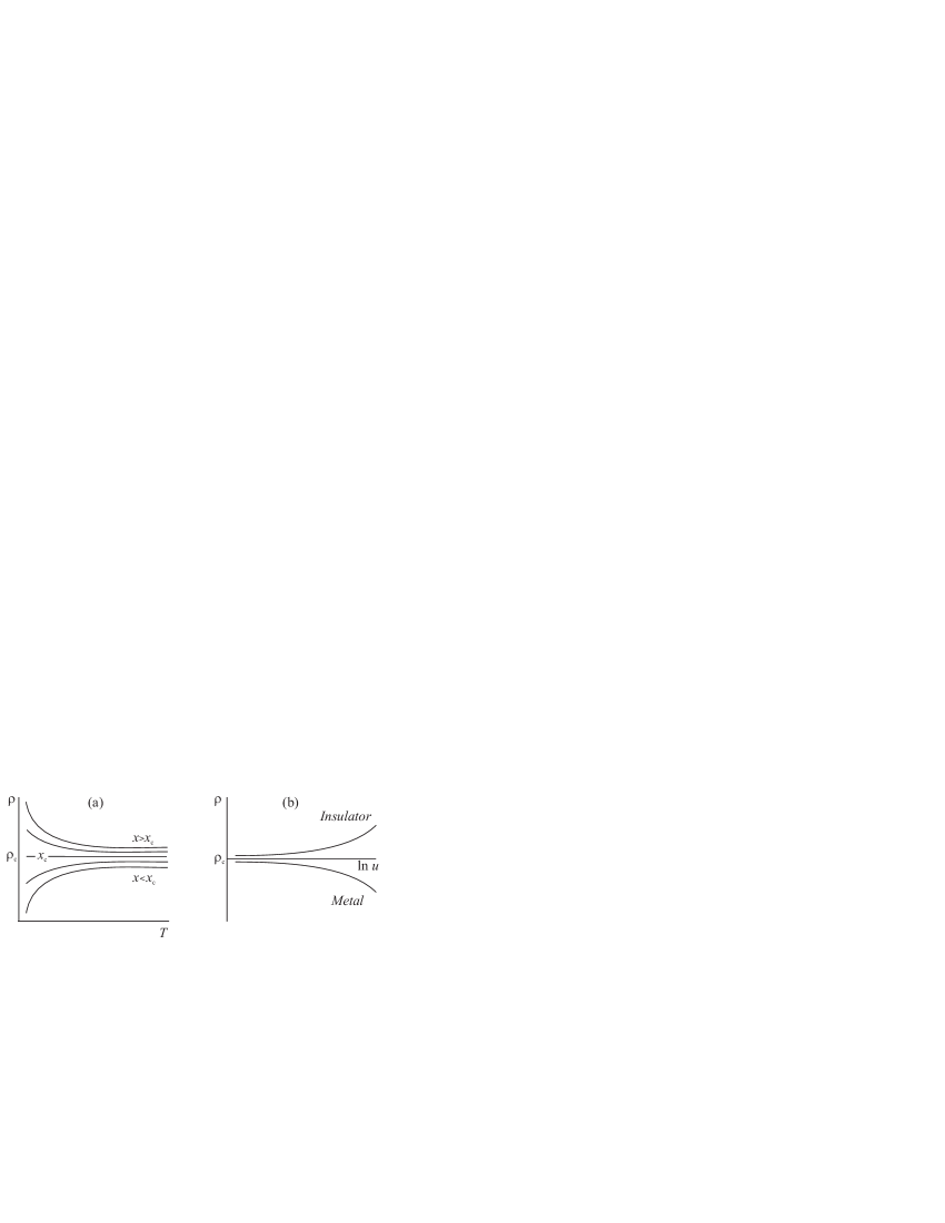
Figure 5: (пїЅ) Temperature dependence of the resistivity $\rho(T)$ at various values of $x$ with the horizontal separatrix $x=x_{c}$. (b) Reduction of the all the $\rho(x,T)$ curves to two curves (34) of the dependence of the resistivity $\rho$ scaling variable (35)

In conclusion of this section, as an example, we present an implication of Eqn (34) for the resistivity of a two-dimensional system. If a quantum phase transition induced by electron localization occurs in a two-dimensional system and manifests itself in the transport properties of this system, we can write

$$d=2:\qquad\rho(x=x_{c})\equiv 1/F(0),\qquad\mbox{i.e.}\qquad\rho(x_{c},T)=\mbox{const}=\rho_{c}.$$ (36)

This implication (a horizontal separatrix in the set of temperature dependences at various values of $x$) is schematically shown in Fig. 5a. We note that it is valid only under assumption (25), which indicates that the correlation length $\xi$ is temperature independent. In general, $\rho(x_{c},T)$ may have a finite slope at the point $T=0$ (cf. below, section 5.3 and Fig. 13).

Usually, with $\delta x$ replaced by the modulus $|\delta x|$, the $\rho(u)$ curve is represented in the form of two branches as a function of $\ln u$ (Fig. 5b). The values of $z\nu$ are then chosen such that these curves fit all the experimental points obtained at various temperatures.

III 3. Flow diagrams for metal–insulator transitions

So far, we have not specified the type of a quantum phase transition. Hereafter, we speak about transitions related to a change in the electron localization, which, in turn, is caused by the degree of disorder in the system. The general theory of quantum phase transitions initially assumes that a control parameter affects the interparticle interaction and that a disorder is not more then a perturbative factor in the initial scheme of quantum phase transitions. Therefore, the applicability of this scheme to metal–insulator transitions, in which the degree of disorder is the main factor and the interaction is a secondary factor, is not obvious a priori.

The fundamental difference between an insulator and a metal is that the electronic states at the Fermi level are localized in an insulator and delocalized in a metal. If an insulator is transformed into a metal due to a change in a certain parameter, the properties of the wave functions at the Fermi level change. The main physical property that is radically different in materials of these two types is the conductivity, i.e., the possibility of carrying an electric current at an arbitrarily weak electric field. This gives a ‘yes–no’ type signature: the conductivity is either zero, $\sigma=0$, or nonzero, though it may be arbitrary small. However, at a finite temperature $T\neq 0$, an insulator also carries a current owing to hopping conductivity. Therefore, the definition of an insulator given above is only related to the temperature $T=0$, and the concept of a metal–insulator transition makes sense only at $T=0$.

That the conductivity $\sigma$ is not a function of the state (because it is realized only under nonequilibrium conditions) is an additional argument against the applicability of the general theory. However, Thouless Thouless noted that the transport properties can be used to characterize the decrease in the wave function of an electron placed at the center of an $L^{d}$ cube in a $d$-dimensional space when it moves toward the edges of the cube. Therefore, in analyzing the behavior of conductance or conductivity near the transition, we actually follow the evolution of wave functions.

Thus, we have every reason to apply the general theory of quantum phase transitions to metal–insulator transitions. However, the first successful version of a theoretical description of metal–insulator quantum transitions b4 was based on the renormalization group theory FiReview borrowed from quantum field theory. The essence of its conclusions, related to systems of noninteracting electrons in a random potential, is illustrated in Fig. 6, which shows the logarithmic derivative of the conductance of a sample with respect to the size $L$,

$$\beta{=}{\frac{\textstyle d\ln y}{\textstyle d\ln L}}{=}\frac{\textstyle L}{\textstyle y}\frac{\textstyle dy}{\textstyle dL}$$

at the temperature T=0 as a function of the conductance $y$,

$$\frac{\textstyle d\ln y}{\textstyle d\ln L}=\beta_{d}(\ln y).$$ (37)

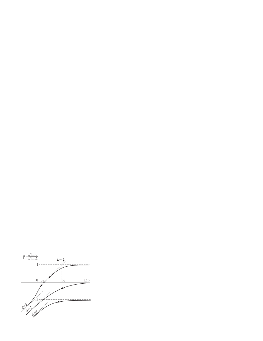
Figure 6: Universal $\beta(\ln y)$ functions for different dimentionalities b4 .

The $\beta_{d}(\ln y)$ curves describe the universal laws of a change in the conductance of the system when its sizes change. The behavior of the system of noninteracting electrons in any material is described by a part of the curve $\beta_{d}$ for the corresponding dimension $d$. The interpretation and method of using these curves are described in detail in review LeeR and book Gant .

For metal–insulator quantum phase transitions, the theory b4 plays the role of an existence theorem. The shape of the $\beta_{d}(\ln y)$ curves and their position in the $(y,\beta)$ plane indicate that these transitions are absent in one- and two-dimensional systems of noninteracting electrons and that in three-dimensional systems, such a transition can occur, with the conductivity of the material changing continuously during this transition. This means that sufficiently large one- and two-dimensional samples should be always insulators at absolute zero whereas a three-dimensional material can be either an insulator or a conductor. Below, we discuss this feature in detail. Here, we note that the $\beta_{d}(\ln y)$ curves are called differential flow diagrams or Gell-Mann–Low curves.

On the one hand, the theory in Sachdev ; QuantRev ; Vojta is more specialized than that in b4 in some respects, because it only describes the vicinity of a quantum transition. On the other hand, the theory in Sachdev ; QuantRev ; Vojta is more universal, because its applicability is not limited by either interaction or a strong magnetic field. Therefore, it is of interest to compare the conclusions of these theories for the systems to which they both can be applied.

IV 4. Three-dimensional electron gas

The possibility of a phase transition in a three-dimensional material follows from the fact that the $\beta_{3}(\ln y)$ curve intersects the abscissa axis $\beta=0$. A certain point on the $\beta_{3}(\ln y)$ curve (an image point) corresponds to the transport properties of a sample of size $L$ made from a certain material (Fig. 7a). If this point is located in the lower half-plane $\beta<0$ the material is an insulator, and the image point shifts to the left as $L$ increases; as a result, the conductance of the sample becomes exponentially small. If this point is located in the upper half-plane $\beta>0$ the image point shifts to the right; as a result, the material is a metal, and its conductance $y$ increases with the size $L$.

The curves in Figs 6 and 7a are scarcely adapted for a direct comparison with experimental data because of a special choice of their coordinate axes. This disadvantage can be partly corrected by integrating the equation

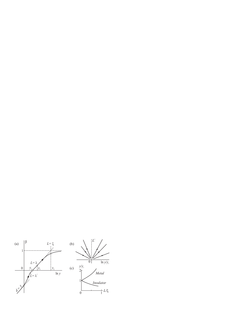
Figure 7: Noninteracting 3D electron gas: (a) differential scaling diagram from b4 (see also Fig. 6); the intersection of the curve $\beta_{3}(\ln y)$ with the abscissa axis $\beta=0$ means existence of a quantum phase transition; (b) flow diagram for a noninteracting 3D electron gas in the vicinity of the transition point; (c) two universal curves of the dependence of the conductance of the 3D system on its size $L$ obtained by scaling

$$\frac{\textstyle d\ln y}{\textstyle\beta_{3}(\ln y)}=d\ln L.$$ (38)

for three-dimensional (3D) systems. Since the left-hand side of differential equation (38) becomes infinite at the point $y=y_{\rm c}$, the curves corresponding to different integration constants decompose into two families: one of them corresponds to an insulator region and the other to a metallic region. To demonstrate this by the simplest way, we restrict ourselves to the immediate vicinity of point $y_{\rm c}$, in which the $\beta_{3}(\ln y)$ curve can be approximated by a straight line,

$$\frac{d\ln y}{d\ln L}=s\ln\frac{y}{y_{c}}$$ (39)

where $s$ is the slope of the line with respect to the abscissa axis. Correspondingly, Eqn (38) can be replaced by linear equation (39). The general solution of linear differential equation (39) is given by

$$\ln\frac{y}{y_{c}}=\left(\frac{L}{\lambda}\right)^{\textstyle s}\ln\frac{y_{\lambda}}{y_{c}},$$ (40)

where $\lambda$ plays the role of the initial condition that fixes the initial point in the $\beta_{3}(\ln y)$ curve; for example, it can be the length $k_{\rm F}^{\,-1}$ determined by the electron concentration. On the metallic side, $k_{\rm F}^{\,-1}$ is equal to the minimum free path length $l_{\rm min}$. The conductance $y_{\lambda}$ corresponds to the point $\lambda$.

Figure 7b shows particular solutions of Eqn (39). If $y_{\lambda}>y_{\rm c}$, we have $\ln y_{\lambda}/y_{\rm c}>0$, the solution is located in the right quadrant, and the conductance $y$ increases with $L$ (metal). If $y_{\lambda}<y_{\rm c}$, we have $\ln y_{\lambda}/y_{\rm c}<0$, the solution is located in the left quadrant, and the conductance $y$ decreases as $L$ increases (insulator). The set of curves in Fig. 7b is called a flow diagram. The arrows in this diagram show the direction of the image point motion when the system size increases. The flow lines corresponding to the particular solutions of Eqn (39) fill both upper quadrants of the $(\ln y_{\lambda}/y_{\rm c},L^{s})$ plane. The boundary between them, the $\ln y_{\lambda}/y_{\rm c}=0$ axis, is called the separatrix; in Fig. 7b, it is indicated by a dashed line.

We extend straight line (39) in Fig. 7a to its intersection with the asymptote $\beta=1$; as a result, we approximate the $\beta_{3}(y)$ curve in the upper half-plane $\beta>0$ by a broken line consisting of segments of two straight lines. The size $L$ which brings the image point to the intersection point is called the correlation length $\xi$. From Eqn (40), we have

$$\xi=\lambda\left(s\ln\frac{y_{\lambda}}{y_{c}}\right)^{-1/s}.$$ (41)

With Eqn(41), we can rewrite general solution (40) as

$$\ln\frac{y}{y_{c}}=\left(\frac{L}{\xi}\right)^{s}$$ (42)

normalize the size $L$ by the length $\xi$ (which is specific for every material), and reduce each of the two families in Fig. 7b to one scaling curve (Fig. 7c).

We make several remarks.

First, Eqns (39)–(42) involve a parameter $s$, which is unknown a priori. However, in the case of a noninteracting 3D-gas, this parameter is either equal to unity or very close to it LeeR . Because $s$ enters all formulas as a factor or exponent, this parameter can be dropped.

Second, the flow lines in Fig. 7b are straight only because we integrated the Gell-Mann–Low equation only in the small vicinity of the transition point. If we integrated the $\beta_{3}(\ln y)$ function over a wide range of its argument $\ln y$ using some model representation, we would obviously obtain curved flow lines.

The third note concerns the role of temperature. The parameter that specifies system motion along the flow lines indicated by arrows in Fig. 7b is the size. If the temperature is taken to be zero (as was assumed until now), this parameter is the sample size $L$. However, we can initially suppose that the system is large, as this is done in the theory of quantum phase transitions Sachdev ; QuantRev ; Vojta . In this case, the limiting size is considered to be the dephasing length $L_{\varphi}$, i.e., the size at which quantum coherence in an electron system is realized. The image point then moves along flow lines in the direction indicated by arrows as the temperature decreases. Because $L_{\varphi}$ depends on the temperature and becomes infinite as $T\rightarrow 0$, this procedure introduces the temperature into the set of physical quantities related to the flow diagram. However, we do not study this relation; based on the ‘existence theorem’ of a quantum transition in a 3D space, we turn to the $(x,T\,)$ phase plane to construct the critical region (see Fig. 8 and compare it with Fig. 4).

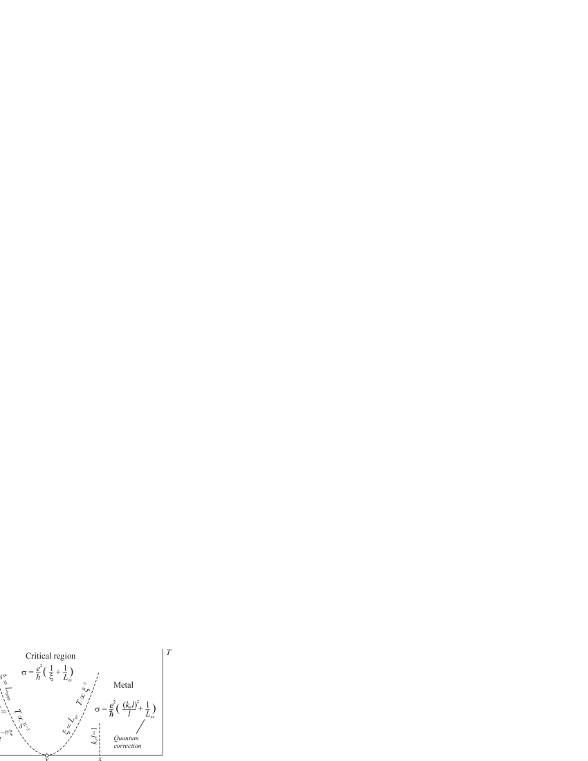
Figure 8: Vicinity of a metal–insulator transition in a noninteracting 3D electron gas in the ($x,T$) phase plane

Let small values of the control parameter $x$ correspond to metallic states. Then, at small $x$ on the abscissa axis, the Drude formula $\sigma=\sigma_{3}=ne^{\,2}l/\hbar k_{\rm F}$ holds, and, at small $x$ and finite $T$, the quantum correction

$$\sigma=\sigma_{3}+\frac{e^{2}}{\hbar}L_{ee}^{-1},\qquad L_{ee}=\sqrt{\hbar D/T}.$$ (43)

is added to $\sigma_{3}$ (here $D$ is the diffusion coefficient). The diffusion length in Eqn (43) is taken to be the length $L_{\rm ee}$ determined by the Aronov–Altshuler effect AA , i.e., by the electron–electron interaction. In other words, we assume that dephasing is caused by internal processes that occur in the electron gas in the time

$$\tau_{ee}=\hbar/T,$$ (44)

without external impacts, such as the electron–phonon interaction (see analogous discussion of the physical meaning of $L_{\varphi}$ in review QuantRev , p. 324).

At any control parameter $x$, another special point $x_{\rm m}$ (the Mott limit) exists on the right of the transition point $x_{\rm c}$. At this special point, we have

$$\sigma(x_{m},T=0)=\sigma_{\rm Mott}=\frac{e^{2}}{\hbar}k_{F}=\frac{e^{2}}{\hbar}\frac{1}{l}.$$ (45)

In the range between $x_{\rm c}$ and $x_{\rm m}$, the Drude formula is invalid: describing conductivity with this formula implies introducing a free path length $l$ that is shorter than the de Broglie wavelength. In this range at $T=0$, $\sigma$ is expressed through the correlation length $\xi$; this corresponds to the general scheme of the theory of quantum phase transitions. As a result, the conductivity along the abscissa axis is expressed as

$$\sigma(T=0)=\left(\frac{e^{2}}{\hbar}\right){\times}\left\{\begin{array}[]{lc}0&\qquad x\geqslant x_{c},\\ 1/\xi&\qquad x_{c}\geqslant x\geqslant x_{m},\\ (k_{F}l)^{2}/l&\qquad x\leqslant x_{m}.\end{array}\right.$$ (46)

To match the last two expressions at $x=x_{\rm m}$, it suffices to set $\xi(x_{\rm m})=l$.

Thus, to describe conductivity in the metallic region, we introduced two parameters, $\xi$ and $L_{\rm ee}$, which have the dimension of length and the properties required for the critical region (they are mutually independent and diverge at the point $x_{\rm c})$. Following Imry , we construct the following interpolation function in the critical region:

$$\sigma=\frac{e^{2}}{\hbar}\left(\frac{1}{\xi}+\frac{1}{L_{ee}}\right)=\frac{e^{2}}{\hbar}\frac{1}{\xi}F\left(\frac{L_{ee}}{\xi}\right)\qquad F(u)=(1+1/u).$$ (47)

Expression (47) matches Eqn (43) on the straight line $x=x_{\rm m}$ and gives the correct values of conductivity in the $x_{\rm c}<x\leqslant x_{\rm m}$ segment at $T=0$. The second form of the function demonstrates that function (47) satisfies general relation (34).

We now move from right to left along the line $T={\rm const}$ (Fig. 4, line $aa$). As long as the quantum correction is relatively small, electron diffusion occurs via scattering by impurities; i.e., it is controlled by the first term in Eqn (43). Therefore, the diffusion coefficient $D$ in $L_{\rm ee}$ is temperature independent. However, when we enter the critical region, $\sigma_{3}$ transforms into $(e^{\,2}/\hbar)\xi^{\,-1}$ and begins to decrease rapidly. Under these conditions, $D$ ceases to be a constant: diffusion is likely to be caused by the electromagnetic-field fluctuations that determine $L_{\rm ee}$; as a result, this diffusion becomes temperature independent. We can then write a set of equations for the $\sigma(T\,)$ and $D(T\,)$ functions with the Einstein relation

$$\left\{\begin{array}[]{l}\sigma={\displaystyle\frac{e^{2}}{\hbar}\left(\frac{1}{\xi}+\sqrt{\frac{T}{\hbar D}}\right)},\\ \sigma=e^{2}g_{F}D\rule{0.0pt}{14.22636pt}\end{array}\right.$$ (48)

used as a second equation. Here $g_{\rm F}$ is the density of states at the Fermi level.

We eliminate $D$ from two equations (48), use that $1/\xi\ll 1/L_{\rm ee}$ near the transition, and obtain the temperature dependence of the conductivity on the right-hand side of the critical region Imry ; AA-Lett ,

$$\sigma(T)=\frac{e^{2}}{\hbar}\left(\frac{1}{\xi}+(Tg_{F})^{1/3}\right)\equiv\alpha+\beta T^{1/3}.$$ (49)

This means that inside the critical region, $L_{\rm ee}$ is given by

$$L_{ee}=(Tg_{F})^{-1/3}.$$ (50)

rather than being determined by Eqn (43). Exactly at the transition, we have $\xi=\infty$ and $\alpha=0$.

Temperature dependence (49) was repeatedly detected in experiments performed on a variety of materials A ; B ; C ; D . Figure 9 shows two examples in which the control parameter is represented by the electron concentration and magnetic field.

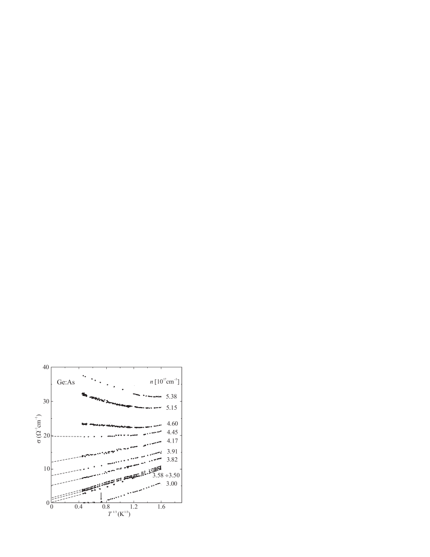
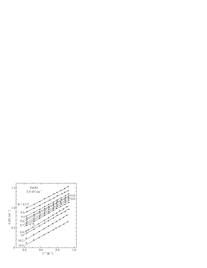
Figure 9: (a) Temperature dependence of the conductivity of Ge:As samples with various level of doping in the region of a metal–insulator transition (from E ); the critical concentration is determined by the extrapolation of the experimental data to $T=0$. b) Temperature dependence of the conductivity of a GaAs sample in various magnetic fields in the region of a metal–insulator transition (from C ); the critical field determined by extrapolation is 9.78 T.

Using condition (32) and Eqn (49), we can write the relation

$$T\propto(g_{F}\xi^{3})^{-1}.$$ (51)

for the right boundary of the critical region. If the relation $\xi\propto(\delta x)^{-1}$ holds (i.e., if $\nu=1$, as is assumed in Fig. 8), the boundary of the critical region is represented by a cubic parabola $T\propto(\delta x)^{3}$. In the general case, we have $\nu\neq 1$ and

$$T\propto(\delta x)^{3\nu}/g_{F}.$$ (52)

A comparison with Eqn (33) demonstrates that in the metal–insulator transition in a 3D system of noninteracting electrons, the dynamic critical index is

$$z=3.$$ (53)

Below curve (52) in the $x_{\rm c}>x>x_{\rm m}$ segment, the conductivity is also described by Eqn (47); however, $L_{\rm ee}$ enters Eqn (47) in the initial form (43) with the diffusion coefficient $D={\rm const}$. Therefore, the temperature dependence of the conductivity in this region should have the form $\sigma(T\,)=\alpha+\beta T^{\,1/2}$.

Up to this point, we have discussed the right-hand side of the phase diagram. The left-hand side of the phase diagram, i.e., the insulator region (where hopping conductivity takes place), also has two characteristic lengths. First, there is the decay length $\xi$ of the localized-state wave functions, $\psi\propto\exp{(-r/\xi)}$. Far from the transition, $\xi$ decreases to the Bohr radius $a_{\rm B}=\kappa\hbar^{\,2}/(m^{\,*}e^{\,2})$ (where $\kappa$ is the dielectric constant and $m^{\,*}$ is the effective electron mass); at the transition, it diverges because the electrons become delocalized. Second, there is the average hopping distance $\overline{r}$. If the hopping conductivity is described by the Mott law, the average hopping distance is Gant

$$\overline{r}=(\xi/g_{B}T)^{1/4}.$$ (54)

The lengths $\overline{r}$ and $\xi$ cannot be used as two independent lengths in the critical region because they are connected by relation (54). However, using $L_{\rm ee}$ determined by Eqn (50), we can rewrite Eqn (54) as

$$\overline{r}=(\xi L_{ee}^{3})^{1/4},$$ (55)

We take into account that expression (50) for $L_{\rm ee}$ does not contain the kinetic characteristics of the electron gas and consider $L_{\rm ee}$ the dephasing length over the entire critical region, including its left-hand side, above the $x_{\rm i}>x>x_{\rm c}$ segment on the abscissa axis. Equation (52) then determines both the right and left boundaries of the critical region. Equations (54) and (55) demonstrate that $\overline{r}=\xi=L_{\rm ee}$ at the left boundary.

The conclusion that $L_{\rm ee}$ can be considered to be the dephasing length over the entire critical region is supported experimentally: as can be seen from Fig. 9, the $\sigma(T\,)$ temperature dependence straighten in terms of the $(T^{\,1/3},\sigma)$ axes, not only on the right-hand side of the critical region but also at values of the control parameter $x<x_{\rm c}$ (e.g., at the electron concentration $n=3\times 10^{17}\,$cm^-3 in Fig. 9). However, the free term $\alpha$ in Eqn (49) becomes negative. This means that we should either suppose that correlation length $\xi$ is negative in the insulator region or (which is formally preferred but is essentially the same) should replace interpolation formula (49) on the left-hand side of the critical region by the formula

$$\sigma(T)=\frac{e^{2}}{\hbar}\left(-\frac{1}{\xi}+\frac{1}{L_{ee}}\right).$$ (56)

As follows from Eqns (55) and (56), we have $\sigma=0$ along the left boundary of the critical region, which means that the conductivity along this boundary is determined up to an exponentially small hopping conductivity.

The hopping conduction mechanism is still operative below the lower boundary of the critical region over the $x_{\rm i}>x>x_{\rm c}$ segment, and the wavefunction decay length is $\xi\gg a_{\rm B}$ rather than $a_{\rm B}$ Castner . Therefore, $a_{\rm B}$ does not enter the expression for the hopping conductivity, and $\sigma$ is expressed in terms of the correlation length $\xi$ (see Fig. 8):

$$\sigma\propto\exp(-\overline{r}/\xi).$$

The $(x,T\,)$ phase diagram in Fig. 8 accumulates the results of the long-term experimental studies of the low-temperature transport properties of conducting systems, namely, the quantum corrections to metallic conductivity, the evolution of electronic spectra during metal–insulator transitions, the temperature dependence of conductivity in the vicinity of the transitions, and hopping conductivity. In essence, this phase diagram was plotted irrespective of the theory of quantum phase transitions Sachdev ; QuantRev ; Vojta in order to reveal the compatibility of all experimental data. Nevertheless, the considerations given above demonstrate that this diagram is absolutely adequate for the concepts following from this theory.

V 5. Two-dimensional electron gas.

5.1 Gas of noninteracting electrons

We now pass to 2D systems. According to the theory by Abrahams et al. [7], a 2D system $(d=2)$ of noninteracting electrons is always an insulator in the sense that localization should inevitably occur in a sufficiently large sample, $L>\xi$, at a sufficiently low temperature, $T<T_{\xi}$, and an arbitrarily small disorder. This statement follows from the fact that flow line $d=2$ in Fig. 6 asymptotically approaches the $\beta=0$ axis and does not intersect it (this line is shown in Fig. 10a). However, in weakly disordered films, the correlation length $\xi$, which bounds the size $L$ below, can be unrealistically large, and the temperature $T_{\xi}$ of the crossover from the region with a logarithmic quantum correction to the conductivity to the region that is characterized by an exponential temperature dependence is, in contrast, too low. These films are called metallic films.

Estimates of $\xi$ and $T_{\xi}$ can be obtained from the assumption LKh that the logarithmically diverging quantum correction $\Delta\sigma$ in the conductivity

$$\sigma=\sigma_{2}+\Delta\sigma=(e^{2}/\hbar)(k_{F}l)-(e^{2}/\hbar)\ln(L_{ee}/l)$$ (57)

is of the order of the classical conductivity $\sigma_{2}$, and hence $\sigma\approx 0$ and

$$\ln(L_{ee}/l)\approx k_{F}l.$$ (58)

The diffusion length $L_{\rm ee}$ over which electron dephasing occurs is determined by Eqn (43). The value of $L_{\rm ee}$ determined from Eqn (58) is defined as the correlation length $\xi$,

$$\xi=l\exp(k_{F}l),$$ (59)

and the temperature

$$T_{\xi}=D\hbar/\xi^{2},$$ (60)

determined from the relation $L_{\rm ee}=\xi$ using Eqn (43) is called the crossover temperature. Of course, the conductivity does not vanish at $T=T_{\xi}$; however, the theory of weak localization is obviously not valid at this temperature, and the resistivity should begin to increase exponentially with decreasing the temperature at $T<T_{\xi}$ in samples of size $L>\xi$.

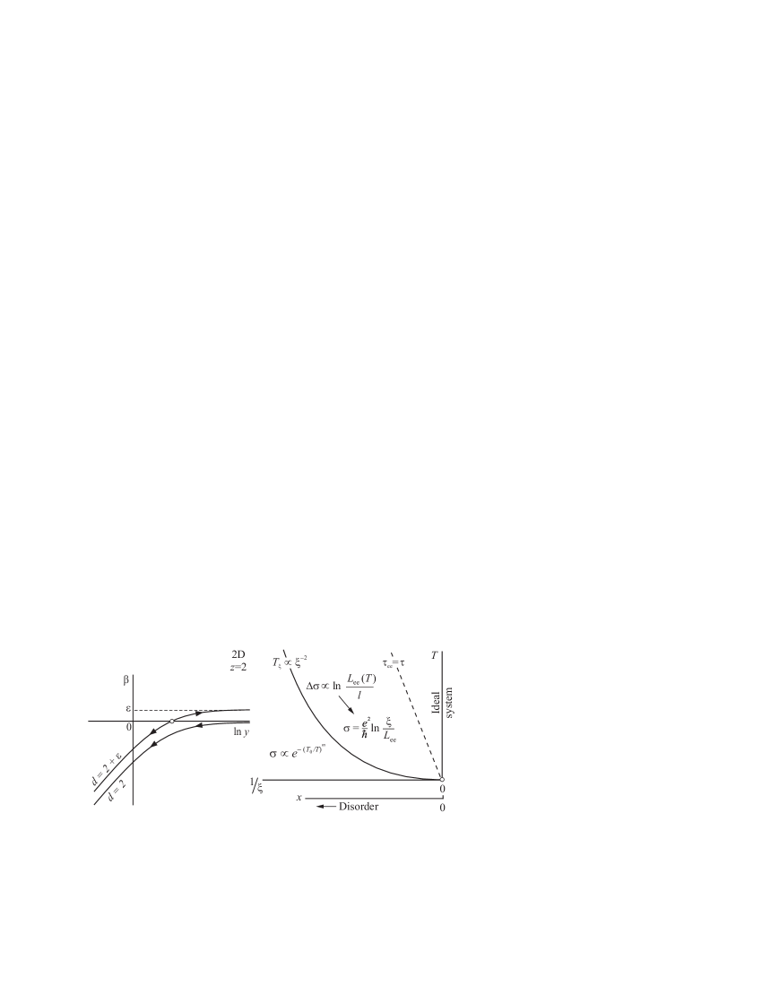
Figure 10: Noninteracting 2D electron gas: (a) differential flow lines for systems with dimension $d=2$ taken from the scaling diagram in b4 (see also Fig. 6) and $d=2+\varepsilon$ (see text), and (b) crossover from the logarithmic temperature dependence of conductivity to its exponential dependence, which can be treated as the boundary of the critical region of a virtual quantum transition (see text)

We now plot function (60) and, for convenience, direct the $1/\xi$ axis to the left (see Fig. 10). As a result, this diagram can be conveniently compared with the diagram for a 3D system shown in Fig. 8. We add an axis and lay off the control parameter $x$ as abscissa; this parameter characterizes the degree of disorder, with $x=0$ corresponding to an ideal system in which a disorder is absent.

It is easily seen that the $T(1/\xi)$ curve in Fig. 10 represents the left-hand side of the phase diagram in the vicinity of a metal–insulator transition in a 3D material (cf. Fig. 8) whose phase transition point is located at the edge of the diagram, at the origin $(T=x=0)$. Curve (60) is then the left boundary of the critical region, and the dynamic critical index is

$$z=2.$$ (61)

Using Eqns (53) and (61), one can conclude that for metal–insulator transitions in systems of noninteracting electrons, the dynamic critical index is equal to the dimension, $z=d$.

Thus, systems with dimension $d=2$ turn out to be boundary systems: a quantum transition is still present in the $(x,T\,)$ phase plane but is shifted toward its corner, to the unreachable point $x=0$. The boundary properties of 2D systems can also be found from the flow diagram in Fig. 6. We imagine that the dimension $d$ is a continuous parameter and can take not only integer values. Straight lines $\beta=d-2$ represent the asymptotics of the flow lines at high values of $y$. Therefore, the flow lines of a system with dimension $d=2+\epsilon>2$ inevitably cross the abscissa axis $\beta=0$, and such systems have a metal–insulator transition (Fig. 10a). As $\epsilon\rightarrow 0$, the transition point shifts toward high conductance and goes to infinity.

This interpretation of the curve in Fig. 10 implies that the domain over the $T\propto(1/\xi)^{2}$ parabola is the critical region of the quantum transition. For 2D systems, only one scaling variable $u$ is retained in Eqn (34) written for the conductivity in the critical region; it is equal to the ratio of two characteristic lengths,

$$\sigma=F(u)\equiv F(L_{\varphi}/\xi).$$ (62)

In this region, however, the conductivity is typically expressed as the difference between the classical conductivity and the quantum correction,

$$\sigma=\sigma_{2}-\Delta\sigma=\frac{e^{2}}{\hbar}\left(k_{F}l-\ln\frac{L_{ee}}{l}\right).$$ (63)

To resolve this apparent discrepancy, let us substitute the expression $l=\xi\exp{(-k_{\rm F}l)}$ from Eqn (59) in the argument of the logarithm in Eqn (63), move the exponent from the logarithm, and obtain

$$\sigma=\frac{e^{2}}{\hbar}\ln\frac{\xi}{L_{ee}}.$$ (64)

The classical conductivity $\sigma_{2}$ cancels and the remaining part depends only on the scaling variable, as it should be in the critical region. Thus, in this regard, our $(x,T\,)$ diagram also satisfies the requirements of the theory of quantum phase transitions.

Expression (64) holds not in the entire ‘quasi-critical’ region $T>T_{\xi}$; moreover, it diverges on the $x=0$ axis. However, near this axis, the elastic mean free path $l\rightarrow\infty$ and the standard expression for $L_{\rm ee}$ lose their meaning because the necessary condition $\tau_{\rm ee}\gg\tau$ is violated. The boundary of the part of the region where Eqn (64) is invalid, $\tau_{\rm ee}=\tau$, is shown in Fig. 10 by a dashed straight line plotted under the assumption that $\tau\propto x^{\,-1}$.

As is shown in Section 5.3, the introduction of interaction can lead to the appearance of a metal–insulator transition in a 2D system. In terms of the phase diagram shown in Fig. 10, this means that the phase transition point shifts from the origin to a point $x_{\rm c}\neq 0$ on the abscissa axis due to a certain cause, and a boundary additionally appears between the critical and metallic regions. Standard expression (63), which was written for the conductivity in the metallic region and was transformed into Eqn (64), was already used for the description of the conductivity in the critical region. This means that the expression for the conductivity in the metallic region should be radically different and that we should expect the appearance of a marginal metal instead of a Fermi liquid. The nature of the electronic states in this hypothetic metal should be rather peculiar, since electrons are assumed to be localized when interaction is turned off Elihu .

5.2. Spin–orbit interaction

The boundary position of 2D systems makes them sensitive to various types of interaction, e.g., spin–orbit interaction or electron–electron interaction, which can cause a phase transition.

We first consider the spin–orbit interaction. This case is convenient because a flow diagram can be plotted using the $(y,\beta)$ axes of the initial diagram shown in Fig. 6. At large $y$, the initial flow line $\beta_{2}(y)$ deviates down from its right asymptote $\beta=0$ because of weak localization, which results in a decrease in the conductivity (Fig. 10a). But the spin–orbit interaction changes the sign of the quantum correction, i.e., changes weak localization into antilocalization. Therefore, the sign of the derivative on the right-hand side of the $\beta_{2}(\ln y)$ curve should change: the curve deviates upward from the asymptote $\beta=0$, goes to the upper half-plane $\beta>0$, and, hence, inevitably crosses the abscissa axis $\beta=0$ and reaches the left asymptote.

Antilocalization was studied in detail both experimentally Berg and theoretically Lark . In the 2D case $(d=2)$, the quantum correction to the conductivity is given by

$$\Delta\sigma_{2}\approx-(e^{2}/\hbar)\int\limits_{\tau}^{\tau_{ee}\rule[-4.2679pt]{0.0pt}{2.84526pt}}\frac{dt}{t}\left(\frac{3}{2}\,e^{-t/\tau_{so}}-\frac{1}{2}\right),$$ (65)

where $\tau$ is the time between elastic collisions, $\tau_{\rm so}\geq\tau$ is the time between spin-flip collisions, and $\tau_{\rm ee}=\hbar/T$ is the dephasing time. The motion of the image point in the flow diagram now depends on two parameters, the conductance $y$ and time $\tau_{\rm so}$. For various values of $\tau_{\rm so}$, Fig. 11 shows the family of flow lines located between two envelope curves. The lower curve is $\beta_{2}(\ln y)$ from the diagrams in Figs 6 and 10. It can be obtained from integral (65) if we set $\tau_{\rm so}=\infty$ in the integrand, and hence the parenthesis in the integrand becomes equal to unity. The upper curve has the same asymptotics; however, its construction implies that $\tau_{\rm so}=\tau$. Then, we have $t\gg\tau_{\rm so}$ over the major portion of the integration range, and the parenthesis is considered to be $-1/2$.

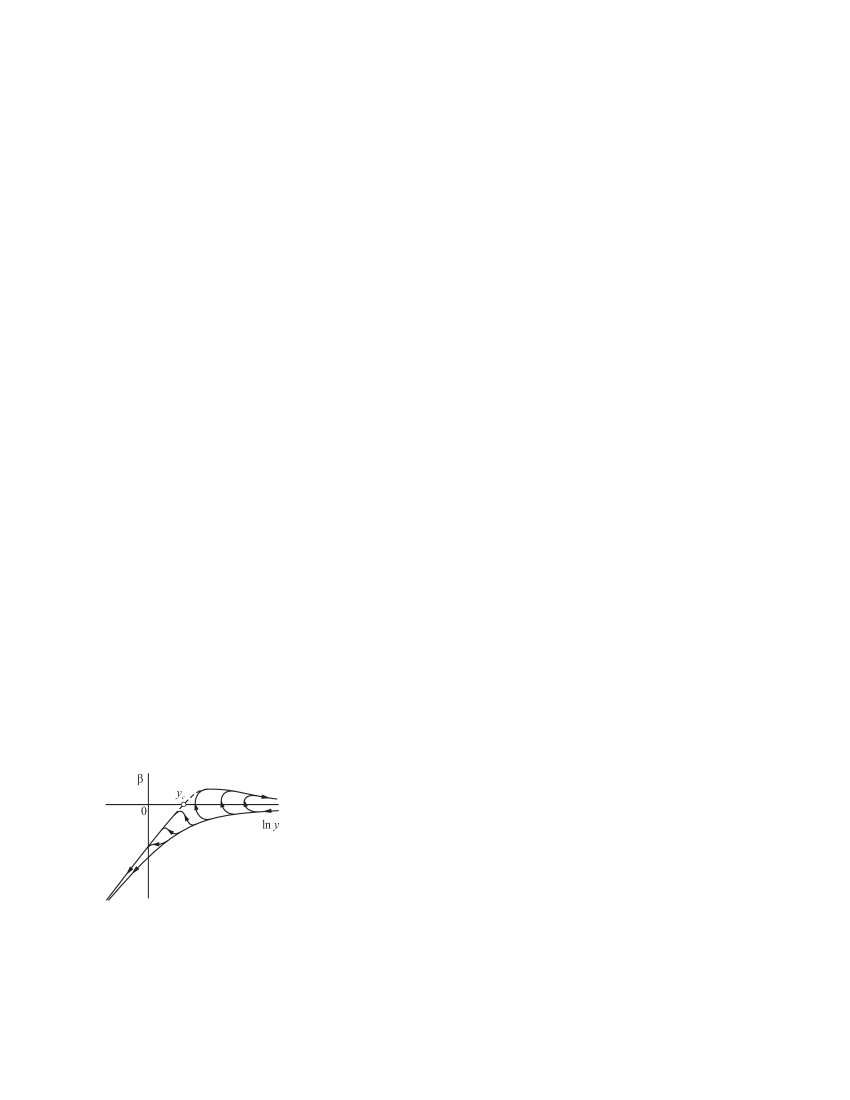
Figure 11: Flow diagram for a 2D electron gas with spin-orbit interaction.

We now take a sample of size $L$ of a material with an intermediate value of $\tau_{\rm so}$,

$$\tau\ll\tau_{so}\ll\infty.$$

The size $L$ bounds the diffusion time $t$ of an electron in a 2D sample until the collision with boundary by the quantity $\tau_{L},t<\tau_{L}\sim\tau(L/l\,)^{2}$. Therefore, to describe weak localization in a sample of size $L$, we must replace the upper integration limit in Eqn (65) with $\tau_{L}$,

$$\tau_{ee}\rightarrow\tau_{L}\equiv\tau(L/l)^{2}.$$

Let $L$ be first very small $(L\,\\ gtrsim1)$ and the temperature $T=0$. Diffusion processes then have no time to develop; electron interference is virtually absent; the conductivity is equal to its classical value; and the image point is on the right on the axis $\beta=0$. As the size $L$ increases to

$$L_{so}=l\sqrt{\tau_{so}/\tau}$$ (66)

spin-flip collisions are insignificant and correction (65) to the conductivity is negative. The image point moves to the left along the lower envelope curve, as in Fig. 10 in the absence of the spin–orbit interaction. When the size $L$ becomes larger than $L_{\rm so}$, integral (65) and $\Delta\sigma_{2}$ change their sign and the image point moves to the upper envelope curve. If this passage occurs at $y<y_{\rm c}$, the film becomes an insulator at $L\rightarrow\infty$ in any case. But if the spin–orbit interaction is strong, $\tau_{\rm so}$ is small and the image point reaches the upper envelope curve at $y>y_{\rm c}$. Then, the image point continues to move along the upper envelope curve toward large $y$, and the film retains its metallic properties as $L\rightarrow\infty$. Thus, a metal–insulator transition could be observed in an experiment with the spin–orbit interaction used as a control parameter. So far, only the transformation of weak localization into antilocalization has been demonstrated this way Berg .

5.3. Gas of interacting electrons

We have to refine what is meant by the absence or presence of the electron–electron interaction. The interaction manifests itself differently in the properties of electron systems; for example, it determines the probability of electron–electron scattering. In the classical theory of metals, electron–electron scattering is considered not to contribute to conductivity, since the total momentum of the electron system and the drift velocity remain the same. When quantum effects are taken into account, this statement becomes invalid because the conductance depends on the dephasing length and electron–electron scattering changes this length. Nevertheless, if the electron–electron interaction affects the conductance only through scattering, the electron system is considered noninteracting, because the interaction affects the conductance as an external action, e.g., scattering by phonons.

Electron–electron scattering is not the only channel of the effect of the interaction on the conductance. The interaction is thought to be not the bare Coulomb interaction but the interaction between ‘dressed’ quasiparticles, i.e., the screened interaction that depends on the electron density, the diffusion coefficient of electrons, and (under certain conditions) the sample size or the quantum coherence length McMillan .

This interaction determines the structure of quantum levels and the ground-state energy, affecting the competition between phases in the vicinity of a phase transition. Electrons are mainly scattered by a screened impurity potential, whose properties depend on the effective electron–electron interaction. This interaction, in turn, depends on the diffusion coefficient and dephasing length, which results in the complex dependence of the effective interaction on all external parameters.

The case of spin–orbit interaction considered in Section 5.2 represents an example of interaction renormalization as the sample size $L$ changes: the spin–orbit interaction is actually turned on only when $L$ becomes larger than the value determined from Eqn (66).

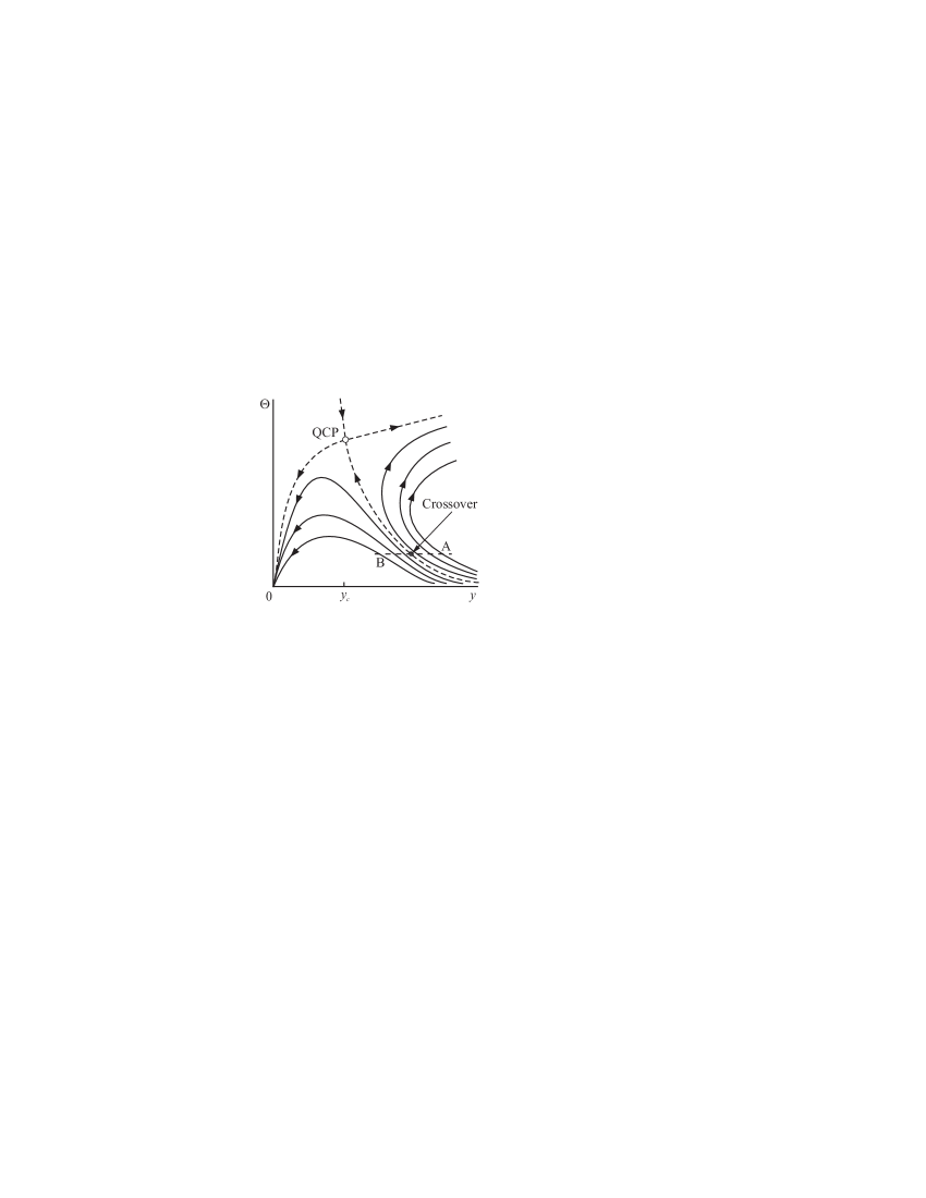
Figure 12: Part of a flow diagram plotted for a 2D electron gas with interaction Fink

As another example, we analyze the picture of possible states in the model with a multivalley electron spectrum developed by Punnoose and Finkel’stein Fink . In this model, a change in $L$ causes changes in both the conductance y and interaction $\Theta$. Therefore, an equation for $\Theta$ is added to Eqn (37). The flow diagram is a result of the solution of these two equations. Figure 12 shows part of this diagram calculated by the authors of Fink in slightly different coordinate axes. The variables were changed to facilitate a comparison of this diagram with those shown in FigsпїЅ6 and 10, although the quantitative information contained in the initial diagram in Fink is lost. The abscissa of the flow diagram shown in Fig. 12 is the conductance. Thus, the abscissa of all the diagrams in Figs 6 and 10 is the same. The ordinate $\Theta$ of the flow diagram in Fig. 12 reflects the effective interaction. A noninteracting electron gas, which was discussed in Section 5.1, corresponds to the straight line $\Theta=0$. As in all previous diagrams (Figs 6–10), the size is the parameter that determines system motion along the flow lines indicated by arrows. This size is given by the sample size $L$ if $T=0$ or by the dephasing length $L_{\varphi}$ (or $L_{\rm ee}$), i.e., the maximum size in which quantum coherence is retained in an electronic system.

The configurations of the flow lines in Fig. 12 clearly display the specific feature of the interaction $\Theta$ that was discussed at the beginning of this section: as the size $L$ or $L_{\varphi}$ changes, the interaction in the system changes (is renormalized), and this change is different in different flow lines. The diagram in Fig. 12 is a two-parameter diagram: two parameters are required to specify the flow line of the image point. The flow lines (trajectories) in this diagram occupy the entire half-plane.

We assume that the position of a point in a flow line is determined by $L_{\varphi}$, i.e., by the temperature. We assume that we are at point A in a flow line, that is metallic because it recedes to the region of high conductivity at $T\rightarrow 0$. We fix the interaction $\Theta$ and vary the conductance $y$; that is, we vary the degree of disorder. This process is shown by a dashed straight line in the diagram. When moving along this line, we can cross the separatrix and reach point B in a flow line that describes an insulator, because it tends to the point $y=0$ as $T\rightarrow 0$. To specify the position of a point in line AB, we can use a single parameter, which is called a control parameter. At another control parameter, the angle of intersection of the separatrix can be different. For example, we can initiate the crossover from a metallic to a nonmetallic flow trajectory by changing the electron concentration and, thus, simultaneously changing the effective interaction $\Theta$ and the conductance.

By changing the control parameter, we can pass from one flow trajectory to another, and, by changing the temperature (size), we can move along a flow trajectory. But because interaction $\Theta$ can change when any of two parameters changes, factorization is absent; that is, we cannot suppose that the length $\xi$ depends only on $\delta x$ and the length $L_{\varphi}$ depends only on temperature. The consequence of this ‘mixing’ of variables is clearly visible in the flow diagram in Fig. 12. As we move along the separatrix toward the quantum critical point (QCP), the conductance decreases and tends to $y_{\rm c}$. Hence, we can draw the following important conclusion, which is qualitatively shown in Fig. 13: the separatrix in the set of temperature dependence is not a horizontal line, as in Fig. 5.

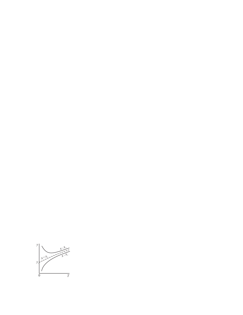
Figure 13: Qualitative scheme for the evolution of the conductance $y(T)$ curves with a control parameter in the model proposed in Fink

An indication of the presence of a metal–insulator transition in a 2D gas was first obtained in the inversion layer of a field-effect transistor on a Si surface Krav . The presence of the transition was questioned for a long time, because is was in conflict with the concepts formulated in b4 and because the transition was not reproduced in other materials. However, the uniqueness of silicon was found to be related to a high electron mobility, which allows performing experiments at a very low electron density, where the electron–electron interaction is especially important. With this fact, it was possible to interpret the experimental data using not the theory in b4 , which was developed for noninteracting electrons, but in accordance with the model in Fink . As a result, the presence of a metal–insulator transition was supported and a finite slope of the separatrix, which was predicted in Fink , was obtained (see Fig. 14a borrowed from Fink1 .

As is seen from the flow diagram in Fig. 12, the finite slope of the separatrix in the set of the temperature dependence of $\sigma$ or $R$ of a system of 2D electrons is controlled by the angle at which the separatrix in the flow diagram approaches the QCP. If the tangent to the separatrix is normal to the abscissa axis at the QCP due to any specific reason, the separatrix in the set of temperature dependence has a zero derivative at $T=0$. Thus, the horizontal position of the separatrix in the set of the temperature dependence of conductivity in the vicinity of the quantum phase transition results from the symmetry of the flow diagram of a certain system and is not an inherent property of all 2D systems. Conversely, a finite slope of the separatrix is not an indispensable consequence of a two-parameter flow diagram.

An inclined separatrix complicates scaling, i.e., the reduction of measurements performed along different flow lines to one universal curve by changing the scales. Nevertheless, the scaling of the resistance $R(T\,)$ data is possible. Figure 14b shows the scaling carried out in the metallic region of the transition displayed in Fig. 14a. The three lower curves in Fig. 14a are replotted in the coordinates $\rho/\rho_{\rm max}$ (instead of $\rho$ ) and $\rho_{\rm max}\ln{(T/T_{\rm max})}$ (instead of $T$; here, $\rho_{\rm max}$ is given in dimensionless units), and the values $\rho_{\rm max}$ and $T_{\rm max}$ correspond to the position of the maximum in each of the experimental curves, which are seen to merge into one curve and to coincide with the theoretical curve. This last curve was plotted using the calculations in Fink and the interaction parameter $\Theta$ determined in the same sample from the magnetoresistance data obtained in a field parallel to the 2D plane.

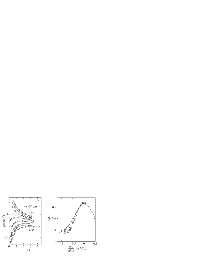
Figure 14: a) Temperature dependence of the resistivity of a 2D gas in a field-effect silicon transistor in a concentration range containing the metal–insulator transition Fink1 . b) Scaling of the three lower curves, which correspond to the concentrations 9.87 ($\square$), 9.58 ($\bigcirc$), and 9.14$\cdot 10^{10}$ cm^-2 ($+$). Theoretical results are shown by a solid line, Fink1

An analogous problem of an inclined separatrix is also often encountered during the experimental processing of the $R_{x}(T\,)$ temperature dependence ($x$ is a control parameter) in the vicinity of superconductor–insulator quantum phase transitions. In Ref. Scaling , a procedure was proposed for the ‘correction’ of the curves via the introduction of the additional linear term

$$R_{x}(T)\rightarrow R_{x}(T)-\alpha T,\qquad\alpha=\left.\frac{\partial R_{x_{c}}(T)}{\partial T}\right|_{T=0},$$ (67)

into each of them to make the separatrix horizontal and for performing subsequent standard scaling for 2D systems using scaling variable (35). The idea of this procedure is to compensate for the slope of the separatrix in a flow diagram. However, the correctness of this procedure has not been proved theoretically.

Figure 15: Critical region in the flow diagram of a 2D electron gas with interaction (indicated by a dotted curve)

Formally, the $(x,T\,)$ phase plane also has a meaning for a two-parameter flow diagram. However, the critical vicinity of the transition can also be directly plotted in the diagram (see Fig. 15). It should be noted that the two-parameter scaling becomes one-parameter in the region adjacent to the separatrix inside the critical region, where flow trajectories are parallel. Indeed, as noted above, one parameter is sufficient to specify the position of a point on line AB, and this parameter does not change when line AB shifts parallel to the separatrix, e.g., to position A₁B₁, since the flow lines are parallel to each other. As we move along the separatrix toward the quantum critical point, near-separatrix trajectories turn aside alternately, and the strip in which the flow trajectories are parallel, as well as the critical region, narrows.

VI 6. Quantum transitions between the different states of a Hall liquid

States in the plateaus of the quantum Hall effect are the specific phase states of a 2D electron gas with special transport properties described by the longitudinal $\sigma_{xx}$ and transverse $\sigma_{xy}$ conductivities

$$\sigma_{xx}\rightarrow 0\quad\mbox{at}\quad T\rightarrow 0,\qquad\sigma_{xy}=i(e^{2}/2\pi\hbar),\qquad i=0,1,2,3...\>.$$ (68)

Such phase states of a 2D electron gas are quantum Hall liquids with different quantum Hall numbers $i$, which are determined by the values of the Hall conductivity $\sigma_{xy}$, Eqn (68), in the plateaus,

$$i=\sigma_{xy}/(e^{2}/2\pi\hbar),\qquad i=1,2,3...\>.$$ (69)

The transitions from one plateau to another induced by a change in the magnetic field or the electron concentration are clearly visible in experimental curves. As can be seen from Fig. 16, $\sigma_{xy}$ jumps are accompanied by narrow $\sigma_{xx}$ peaks. These jumps are quantum phase transitions, and they should fit both theoretical versions compared in Section 5.

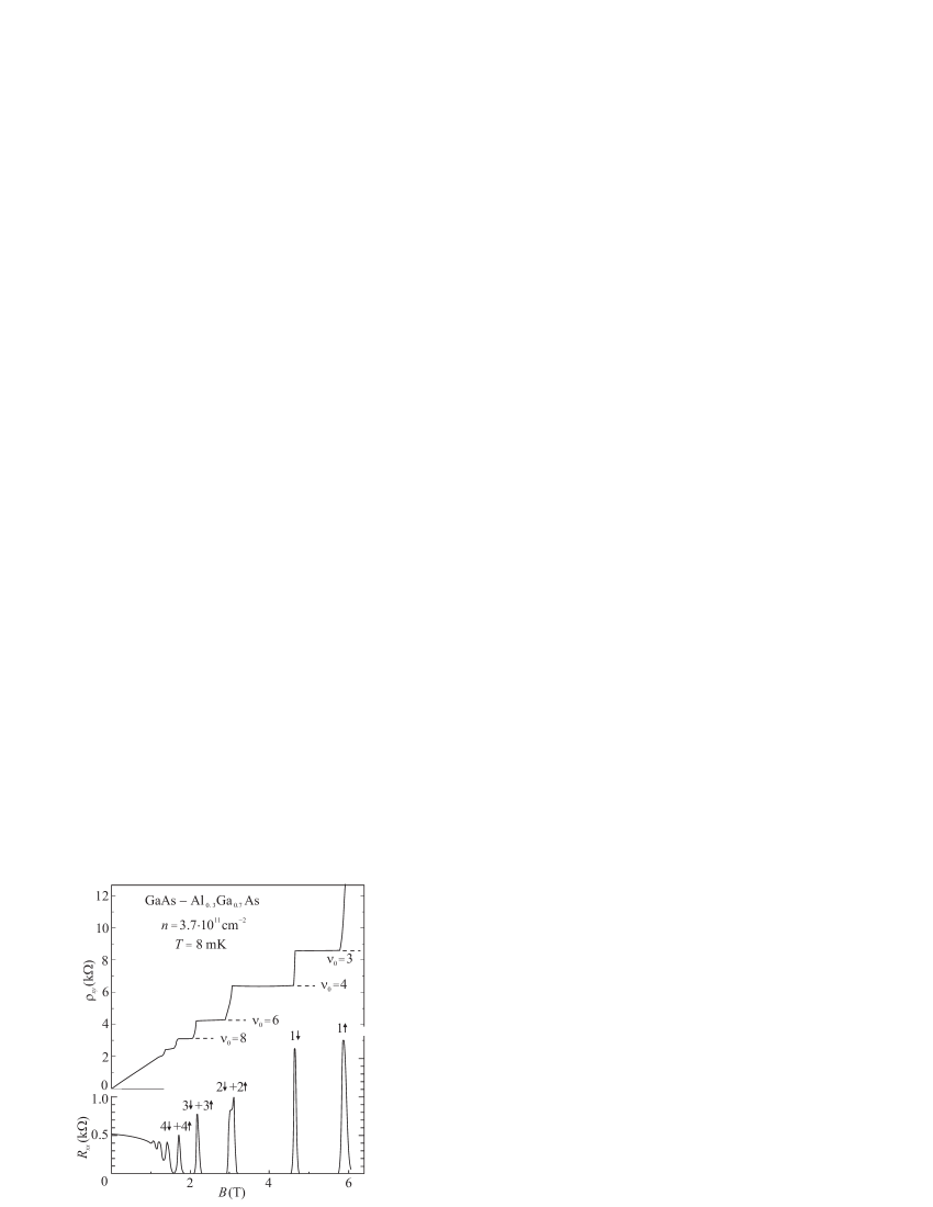
Figure 16: The magnetoresistance $R_{xx}$ and the Hall resistivity $\rho_{xy}$ versus the magnetic field $B$ in a GaAs–Al_xGa_1-xAs heterostructure at $T=8$ mK K1 . The electron density in the 2D layer is $3.7\cdot 10^{11}$ cm^-2, and the mobility is $\mu=4.1\cdot 10^{4}$ cm²/V$\cdot$s.

Figure 16 only displays the plateaus of the integer quantum Hall effect, which is considered below. The integer quantum Hall effect can also be realized in a noninteracting electron gas; therefore, it can be described without regard for interaction.

To construct the flow diagram of a 2D system of noninteracting electrons in a strong magnetic field, we need two conductance components that are equivalent to conductivity components $\sigma_{xx}$ and $\sigma_{xy}$. Correspondingly, Eqn (37) transforms into the set of two equations

$$\begin{array}[]{c}\frac{\textstyle d\ln\sigma_{xx}}{\textstyle d\ln L\rule{0.0pt}{8.53581pt}}=f_{1}(\sigma_{xx},\sigma_{xy}),\\ \frac{\textstyle d\ln\sigma_{xy}}{\textstyle d\ln L\rule{0.0pt}{8.53581pt}}=f_{2}(\sigma_{xx},\sigma_{xy})\rule{0.0pt}{22.76219pt},\end{array}$$ (70)

When eliminating the variable $L$ from two equations (70), we find a relation between $\sigma_{xx}$ and $\sigma_{xy}$, which can be displayed as curves in the $(\sigma_{xy},\sigma_{xx})$ plane Khmel1 . These curves make up a flow diagram for a 2D system of noninteracting electrons in a strong magnetic field (Fig. 17). The flow lines in this diagram are separated by separatrices periodically repeated along the $\sigma_{xy}$ axis. This diagram is again a two-parameter diagram, but due to a strong magnetic field rather than to interaction. As in the previous flow diagrams, we can move along arrows in flow trajectories by either increasing the sample size $L$ or decreasing the temperature at large $L$, i.e., increasing $L_{\varphi}$.

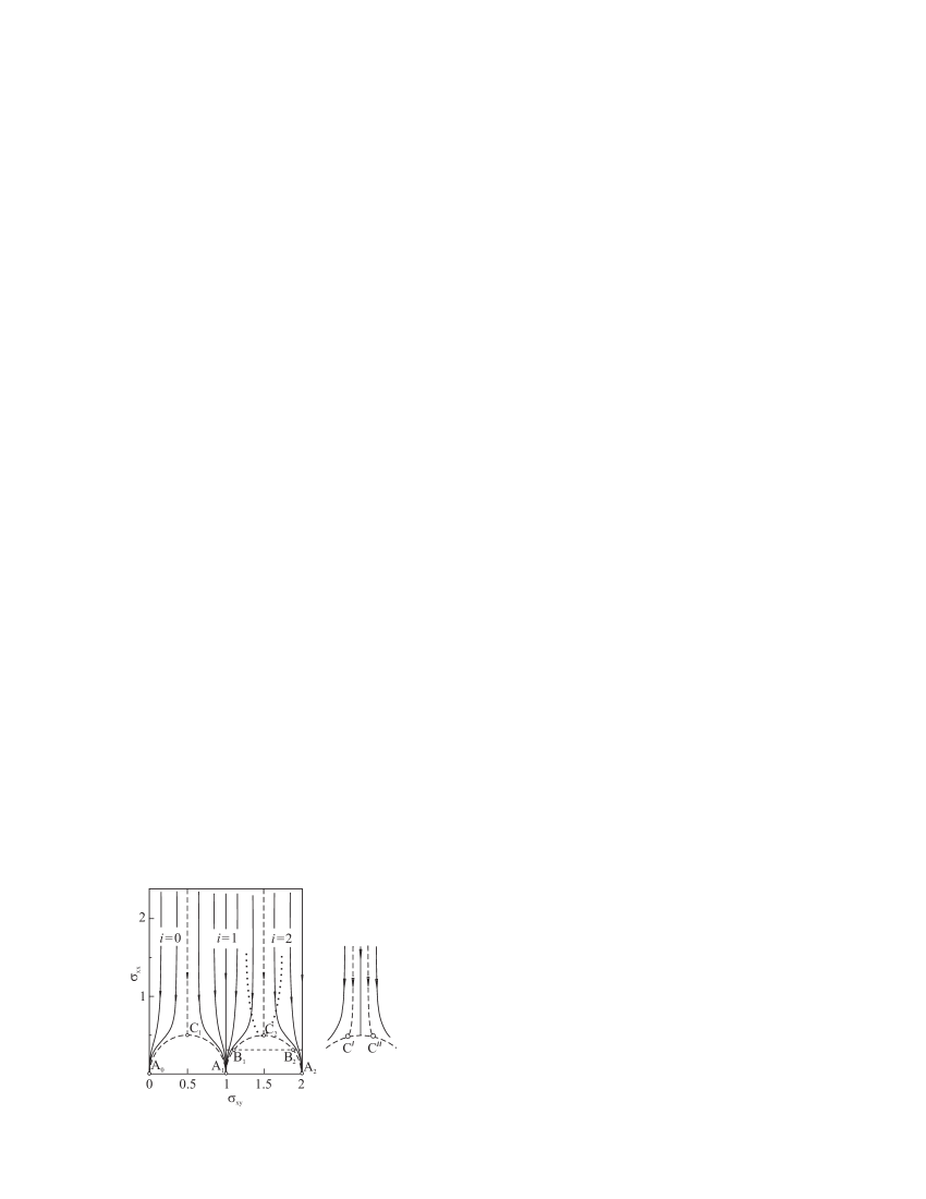
Figure 17: Flow diagram for a 2D electron gas in a strong magnetic field Khmel1 . The coordinates are represented by the conductivity tensor components $\sigma_{xy}$ and $\sigma_{xx}$ in the dimensionless units $e^{2}/2\pi\hbar$. Separatrices are indicated by dashed lines. A_i are stationary singular points, C_i are unstable singular points, which are quantum transition points similar to QCP in Fig. 12. The dashed line indicates the critical region near C₂. Horizontal dashed line $B_{1}$–$B_{2}$ indicates the image point hopping as the control parameter changes. The right-hand side of the figure shows the hypothetical flow diagram that corresponds to a split phase transition and the appearance of a metallic phase

In the region below points ${\rm C}_{i}$, the separatrix is split such that two equivalent points located at the same height $({\rm B}_{1}$ and ${\rm B}_{2})$ appear in it. The flow lines inside the semicircles in Fig. 17 are omitted because they are thought to exist separately from the flow lines outside these semicircles: as the control parameter in the region below points ${\rm C}_{i}$ changes, the motion leads to a hop between points $({\rm B}_{1}$ and ${\rm B}_{2})$ and to a sharp increase in $\sigma_{xy}$. Strictly speaking, the transfer should occur along a line located outside the semicircle and bypassing the point ${\rm C}_{i}$ above. However, for simplicity, it is indicated by a horizontal dashed line.

The control parameter in the quantum Hall effect regime is usually given by the electron concentration or the magnetic field. Their effect on the state of a real system depends on the random field of impurities and other defects, which transforms discrete Landau levels into minibands and specifies the energy structure and the character of wave functions in them. Because a magnetic field determines the magnetic length $r_{B}=\bigl{(}\hbar c/|e|B\bigr{)}^{1/2}$ as a characteristic scale, we can speak about two limiting types of random potential, a potential with large-scale fluctuations of characteristic sizes $\zeta\gg r_{B}$ and a short-range potential with $\zeta\ll r_{B}$. In the long-period potential model, an energy value $\varepsilon_{\rm c}$ exists near the center of each Landau miniband such that a delocalized electron wave function corresponds to this value. If the wave function is strictly delocalized only at $\varepsilon_{\rm F}=\varepsilon_{\rm c}$ and the random field lifts the degeneracy of energy levels, a smooth change in the electron concentration produces a jumplike transformation of the system from one phase state into another through an isolated energy state with a delocalized wave function at the Fermi level. This behavior is implied in the flow diagram in Fig. 17, where each isolated metallic state corresponds to a peculiar separatrix.

The actual width $\delta\varepsilon$ of the energy range with delocalized wavefunctions depends on finer processes, such as tunneling between two semiclassical trajectories that are close to each other in the vicinity of the saddle point (magnetic breakdown). In essence, $\delta\varepsilon$ is the energy uncertainty of any delocalized state. Another source of increasing the $\delta\varepsilon$ range is the finiteness of the lengths $L$ and $L_{\varphi}$. If the $\delta\varepsilon$ range is finite, a separatrix is split into two parallel lines and the phase transition is split into two transitions: a metallic state with a partly filled layer of extended states at the Fermi level should appear between two Hall-liquid states whose indices $i$ differ by unity. The corresponding hypothetical flow diagram is shown on the right-hand side of Fig. 17.

At first glance, it seems that experiment can distinguish between these two hypothetical possibilities. For definiteness, we assume that the electron concentration $n$ changes in experiment (considerations for a change in the magnetic field are similar). As the concentration changes, the Fermi level moves along the energy scale. When states at the Fermi level are delocalized, the $\sigma_{xx}$ conductivity is finite, and the $\sigma_{xy}$ conductivity is in the intermediate region between two plateaus. Therefore, the temperature dependence of the concentration range of the intermediate region (i.e., the $\sigma_{xx}$ peak width, the $\partial\sigma_{xy}/\partial n$ derivative at the center of the intermediate region, etc.) extrapolated to $T=0$ must determine the energy range $\delta\varepsilon$ of the delocalized states.

However, the experimental results were found to be ambiguous. On the one hand, the comprehensive experiments in D1 ; Balaban give a finite value of $\delta\varepsilon$. For example, Fig.18 shows the transition width measured from the $\rho_{xx}$ resistivity peak width of a 2D gas in the GaAs/AlGaAs heterojunction. The measured function is seen to be reliably extrapolated to $\Delta B_{0}\approx 0.35$ as $T\rightarrow 0$. However, as we see below, many experiments give the opposite result: as the temperature decreases, the transition width tends to zero (see, e.g., Fig. 20). The factor that determines $\delta\varepsilon$ has not yet been revealed. In any case, there is no unique relation between $\delta\varepsilon$ and mobility. The statistical characteristics of the random potential, which are poorly controlled, are likely to play a key role.

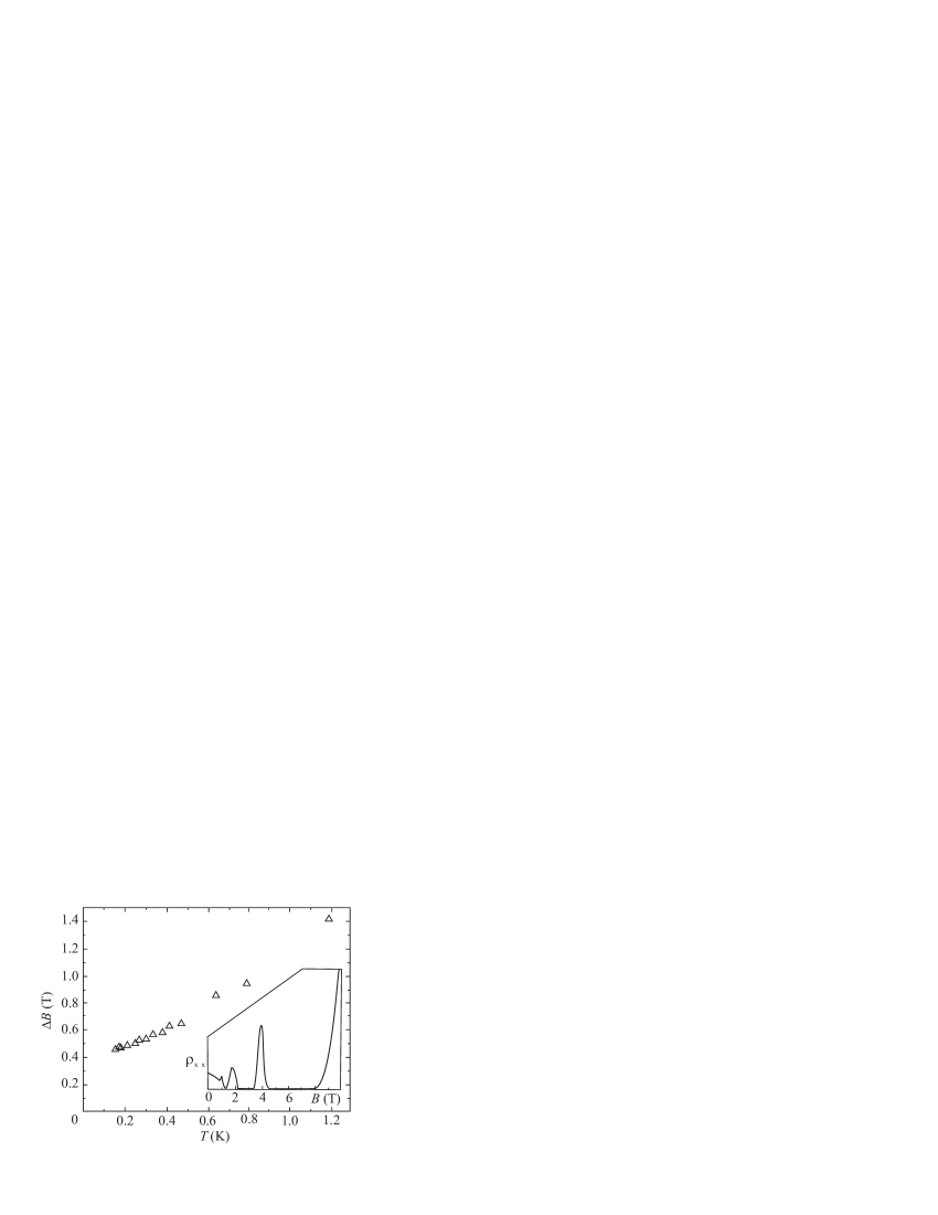
Figure 18: Temperature dependence of the peak width of the longitudinal resistivity $\rho_{xx}$ of a 2D electron gas in the GaAs/AlGaAs heterojunction during the $2\rightarrow 1$ transition in the magnetic field about 4 пїЅ Balaban . The carrier mobility and concentration at $T=1.5$ K are $\mu=34000$ cm²/V s and $n=1.4\cdot 10^{11}$ cm^-2. The inset shows $\rho_{xx}(B)$ curve recorded at 150 mK

We now move to experiments that do not exhibit a finite energy layer with delocalized states. Although the flow diagram of $i\rightarrow i+1$ transitions between different states of a Hall liquid has two parameters (see Fig. 17), it is symmetric with respect to both the $\sigma_{xy}=(i+1/2)(e^{\,2}/2\pi\hbar)$ and $\sigma_{xy}=i(e^{\,2}/2\pi\hbar)$ axes. Therefore, we may use the version of the general theory of quantum phase transitions that is based on Eqns (25), (26) and assumes that scaling formulas of type (34) are valid. As far as we consider only 2D electronic systems, all resistances have the same dimension [$\Omega$] and must have the form

$$R_{uv}=F_{uv}(L_{\varphi}/\xi)=F_{uv}\left(\frac{\delta x}{T^{1/z\nu}}\right),$$ (71)

in the vicinity of the transition. Here, the $u$ and $v$ subscripts stand for the $x$ and $y$ coordinates, $F_{uv}$ is an unknown function, and the argument of the arbitrary $F$ function is written using the last form in Eqn (35).

In contrast to the case of metal–insulator transitions, we analyze experimental results instead of calculating or predicting the values of $\nu$ and $z$. As an example, Fig. 19 shows the magnetic-field dependence at various temperatures of the longitudinal $R_{xx}$ and transverse $R_{xy}$ resistances of a Hall bar in a GaAs-based heterostructure Tsui .

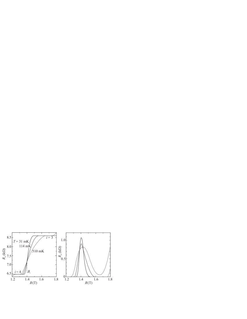
Figure 19: Transverse $R_{xy}$ and longitudinal $R_{xx}$ resistances of an Al_xGa_1-xAs$-$Al_0.33Ga_0.67As heterostructure, $x=0.85\%$, at various temperatures. The critical magnetic field of the 4-3 transition determined from the point of intersection of the $R_{xy}(T)$ curves is $B_{c}=1.40$ T, Tsui

According to Eqn (71), the scaling variable

$$u=\delta x/T^{1/z\nu}$$ (72)

is identically zero at all temperatures in the case where the control parameter takes a critical value; correspondingly, we have

$$R_{uv}(x_{c},T)={\rm const}.$$ (73)

Therefore, separatrix (73) must be horizontal, and all isotherms $R_{uv}(x,T={\rm const})$ must intersect at one point $x=x_{\rm c}$. This is the first test of the applicability of Eqn (71).

We first focus on the $R_{xy}(T\,)$ curves. As is seen from Fig. 19, the $R_{xy}(T\,)$ isotherms obtained for an Al_xGa_1-xAs–Al_0.33Ga_0.67As heterostructure with $x=0.85\%$ Tsui do intersect at one point, $B_{\rm c}=1.40\,$T. Near the intersection point, all the $R_{xy}(T\,)$ curves can be expanded into a series and replaced by straight lines $(\partial R_{xy}/\partial B)_{B_{\rm c}}(B-B_{\rm c})$. As the slopes of these lines are changed from $(\partial R_{xy}/\partial B)_{B_{\rm c}}$ to $(\partial R_{xy}/\partial B)_{B_{\rm c}}/T^{\;\kappa}$, where $\kappa=1/z\nu$, all the straight lines must merge into one line. The choice of the value of $\kappa$ at which the relation

$$(\partial R_{xy}/\partial B)_{B_{c}}(T)/T^{\kappa}={\rm const},$$ (74)

holds is the second step in the application of the scaling procedure, and the possibility of this choice is the second condition for the applicability of the theory. To choose $\kappa$, we plot $(\partial R_{xy}/\partial B)$ versus $T$ on a $\log\!-\!\log$ scale (Fig. 20).

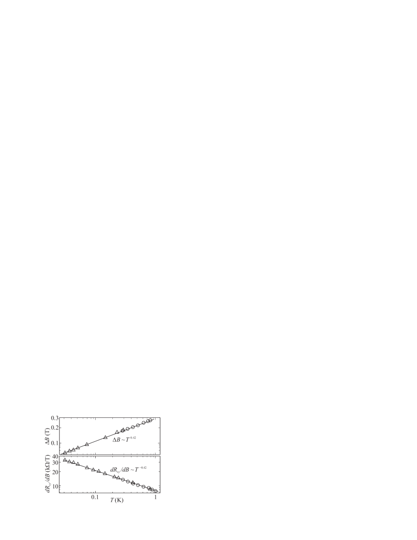
Figure 20: Determination of the critical index $\kappa=1/z\nu$ for transition 4-3 using the $R_{xx}(T)$ peak width (a) and matching the slopes of the intersecting $R_{xx}(T)$ curves (b). The data were obtained from the sample used for Fig. 19 in a dilution refrigerator (triangles) and a liquid ³He cryostat (circles) [33]

Formally, Eqn (71) can be applied to both longitudinal ($R_{xx}$) and transverse ($R_{xy}$) resistances. However, the peak height depends on the temperature; that is, the point of the maximum does not satisfy condition (73). Leaving aside the reasons for this fact, we can use the longitudinal resistance data for scaling analysis by accounting for the integral property of the $R_{xx}(B)$ functions in the vicinity of the transition, namely, the peak half-width $\Delta B$ determined by a certain algorithm. In Fig. 20, $\Delta B$ is determined as the distance between the two maxima of the $(\partial R_{xx}/\partial B)$ derivative.

As can be seen from Fig. 20, an analysis of both families of the functions gives the same value of the critical index $\kappa=0.42$, which is an additional argument for our scaling procedure.

This value of the critical index $\kappa=0.42$ was repeatedly obtained in heterostructures made from various materials. However, contrary to expectations, this value is not universal: other values in the range from 0.2 to 0.8 were also detected in a number of experiments on various heterostructures. This scatter calls for explanations, since scaling relations and critical indices are usually universal.

At $T=0$, transition occurs when the condition $\varepsilon_{\rm F}=\varepsilon_{\rm c}$ is satisfied and therefore the difference $\delta\varepsilon=|\varepsilon_{\rm F}-\varepsilon_{\rm c}|$ is the only ‘internal’ control parameter of the system, with the correlation length $\xi$ depending on it in accordance with a power law:

$$\xi\propto(\delta\varepsilon)^{\nu_{1}}.$$ (75)

From this standpoint, the magnetic field $B$ or the 2D electron concentration $n$, which depends on the gate voltage $V_{\rm g}$, are ‘external’ control parameters $x$,

$$\delta x\equiv|B_{c}-B|\propto(\delta\varepsilon)^{\nu_{2}}\qquad\mbox{or}\qquad\delta x\equiv|n_{c}-n|\propto|V_{gc}-V_{g}|\propto(\delta\varepsilon)^{\nu_{2}}.$$ (76)

In both cases, the exponent $\nu_{2}$ is the same. This is supported by the fact that the $R_{uv}(B)$ and $R_{uv}(V_{\rm g})$ experimental curves recorded using the same sample under equivalent conditions differ only in the scales on the abscissa axis. Eventually, we can write Eqn (25) as

$$\xi\propto(\delta x)^{\nu}\qquad(\nu=\nu_{1}\nu_{2}),$$ (77)

where the relation between the control parameter $\delta x$ and the correlation length $\xi$ consists of the following two links: $\xi$ depends on the position of the Fermi level $\varepsilon_{\rm F}$ with respect to the delocalized level $\varepsilon_{\rm c}$, and the difference $\varepsilon_{\rm F}-\varepsilon_{\rm c}$, in turn, depends on $\delta x$. Correspondingly, according to Eqn (77), the index $\nu$ turns out to be the product of $\nu_{1}$ and $\nu_{2}$. The relation between $\xi$ and $\delta\varepsilon$ and the related index $\nu_{1}$ are likely to be universal and the same for all transitions between different quantum Hall liquids. But the index $\nu_{2}$ is determined by the density of states $g(\varepsilon)$ in the vicinity of the energy $\varepsilon_{\rm c}$ and, hence, depends on the specific features of the random potential; this potential can be long- or short-range, statistically symmetric or asymmetric with respect to the mean value, and so on. The authors of Tsui , whose curves are used in this section, just studied the effect of specific features of the random potential on $\kappa$.

The $\Delta B(T\,)$ curve in Fig. 20 differs radically from the curve in Fig.18; in the latter case, a free term $\Delta B_{0}$ was introduced for the experimental data to be approximated by a power function. Nevertheless, we can also perform scaling analysis of the experimental data in this case using the second hypothetical version of the flow diagram (see Fig. 17). For this interpretation, the presence of the $\Delta B_{0}$ term means that in the $2\Delta B_{0}$ range of the control parameter $B$, the image point in the flow diagram moves across the metallic-phase corridor and falls on a separatrix not at $B_{0}$ corresponding to a maximum of $\sigma_{xx}(B)$ and the derivative $\partial\sigma_{xy}/\partial B$ but at $B_{0}+\Delta B_{0}$. This problem is discussed in detail in review Shash . Here, we only note that Fig. 18 actually contains this scaling analysis. By extrapolating the $\Delta B(T\,)$ dependence to $T=0$, we can determine the delocalized-state layer width in units of magnetic field $2\Delta B_{0}$ and find that $\Delta B(T\,)-\Delta B_{0}$ depends linearly on $T$. This means that $\kappa=1$ in this experiment. The same value of $\kappa$ was obtained earlier in D1 .

VII 7. Conclusion

All the considered cases of metal–insulator transitions were found to be adequately described by flow diagrams. The list of theoretical works that have successfully used this technique begins with work b4 , where a theoretical model for noninteracting electrons in a zero magnetic field was developed. The last achievement in this field is the construction of a flow diagram for a 2D model system of interacting electrons and the demonstration of the possibility of a metal–insulator transition in this system .

As regards the general theory of quantum phase transitions, a phase transition in a 3D system of noninteracting electrons demonstrates that, in principle, this theory can be used to describe localized–delocalized electron transitions. Neither conductance, which is used as a physical quantity specifying the state of the system, nor disorder, which is the main control parameter, are substantial obstacles for this theory. However, as usual, various particular cases require theoretical versions of various degrees of complexity. For example, the version described in this review cannot be applied to the model proposed in Fink .

The relative role and possibilities of both theoretical approaches are demonstrated when the integer quantum Hall effect is described. The flow diagram in Fig. 17 is very convenient for the discussion of the types of transitions that are possible in a system and for the formulation of questions to be experimentally checked. Many of these questions are still open. For example, it is unclear which of the versions of the flow diagram in Fig. 17 is realized in reality and whether the transition between the states with quantum indices $i$ and $i\pm 1$,

$$i\rightleftarrows i\pm 1,$$ (78)

is split [$i$ is determined by Eqn (69)). There are also problems related to the topology of the flow diagram. According to Fig. 17, transitions where quantum number $i$ changes by more than unity are impossible Kiv ; Huck10 . However, when theorists interpret many experimental data, they state that such transitions occur (see, e.g., review Shash and the references therein).

The general theory of quantum phase transitions does not consider the problem of the relative position of various transitions in the phase plane. This theory describes the critical vicinity of one certain transition. Proceeding from the assumptions that (a) a transition exists and (b) the factorization $\xi=\xi(\delta x)$, $L_{\varphi}=L_{\varphi}(T\,)$ occurs in its critical region, the resistivity can be described by Eqns (34)–(36) (see Sections 2.3 and 5.3). Then, the transition point $x=x_{\rm c}$ and critical indices can be determined by processing the $R(x,T\,)$ curves. This procedure was performed in paper Tsui , which was discussed in Section 6. The value of the results obtained in Tsui becomes clear after the questions formulated above and following from flow diagrams are answered.

Acknowledgments

We thank A. Finkel’shtein and D. Khmel’nitskii for the useful discussions. This work was supported by the Program for the Support of Leading Scientific Schools (project no. NSh-5930.2006.2) and the Russian Foundation for Basic Research.

References

- (1) S.Sachdev, Quantum Phase Transitions (Cambridge University Press, Cambridge 2000)
- (2) S.L.Sondhi, S.M.Girvin, J.P.Carini, and D.Shahar, Continuous quantum phase transitions, Rev.Modern Phys. 69, 315 (1997)
- (3) T.Vojta, Quantum phase transitions, in: K.H. Hoffmann and M. Schreiber (Eds) Computational Statistical Physics, Springer, Berlin (2002); cond-mat/0010285
- (4) D.J.Thouless, Phys. Rep. 13C, 93 (1974)
- (5) A.Z.Patasinskii and V.L.Pokrovskii, Fluctuation Theory of Phase transitions. (oxford: Pergamon Press) 1979
- (6) N.Goldenfeld, Lectures on Phase Transitions and the Renormalization Group (Addison-Wesley, Reading, 1992)
- (7) E.Abrahams, P.W.Anderson, D.C.Licciardello, and T.W.Ramakrishnan, Phys.Rev.Lett. 42, 673 (1979)
- (8) M.E.Fisher, Renormalization group theory: its basis and formulation in statistical physics. Rev. Modern Phys. 70, 653 (1998)
- (9) P.A.Lee and T.V.Ramakrishnan, Disordered electronic systems, Rev. Modern Phys. 57, 287 (1985)
- (10) V.F. Gantmakher, Electrons and Disorder in Solids (Oxford University Press) 2005
- (11) B.I.Altshuler and A.G.Aronov. Electron-electron interaction in disordered conductors, in Electron-electron Interactions in Disordered Systems. (Eds.: A.L.Efros and M.Pollak). North-Holland, 1985
- (12) Y.Imry, J.Appl.Phys. 52, 1817 (1981)
- (13) B.I.Altshuler and A.G.Aronov, JETP letters 37, 410 (1983)
- (14) B.W.Dodson, W.L.McMillan, J.M.Mochel, and R.C.Dynes, Phys.Rev.Lett. 46, 46 (1981)
- (15) Y.Imry and Z.Ovaduahu, J.Phys.C 15, L327 (1982)
- (16) M.C. Maliapaard, M.Pepper, R.Newbury, and G.Hill, Phys.Rev.Lett. 61, 369 (1988)
- (17) V.M.Teplinskii, V.F.Gantmakher, and O.I.Barkalov, JETP 74, 905 (1992)
- (18) I.Shlimak, M.Kaveh, R.Ussyshkin, et al., Phys.Rev.Lett. 77, 1103 (1996); J.Phys.: Cond.Matt. 9, 9873 (1997)
- (19) T.G.Castner. Hopping conduction in the critical regime approaching the metal-insulator transition, in Hopping Transport in Solids (Eds.: M.Pollak and B.Shklovskii). North-Holland, 1985
- (20) A.I.Larkin and D.E.Khmel’nitskii, JETP 56, 647 (1982)
- (21) V. Dobrosavljevic, E. Abrahams, E. Miranda, and S. Chakravarty Phys. Rev. Lett. 79, 455 (1997)
- (22) G.Bergmann, Phys.Rep. 107, 1 (1984)
- (23) S.Hikami and A.I.Larkin, Y.Nagaoka, Progr.Theor.Phys. 63, 707 (1980)
- (24) W.L. McMillan Phys.Rev. B 24, 2739 (1981)
- (25) A.Punnoose and A.Finkel’stein, Science 310, 289 (2005)
- (26) S.V.Kravchenko, G. V. Kravchenko, J. E. Furneaux, V. M. Pudalov and M. DпїЅIorio, Phys.Rev. B 50, 8039 (1994)
- (27) S.Anissimova, S.V.Kravchenko, A.Punnoose, A.Finkel’stein, and T.M.Klapwijk, Nature-Physics 3 707 (2007); cond-mat/0609181
- (28) V.F. Gantmakher, M.V. Golubkov, V.T. Dolgopolov, G.E. Tsydynzhapov, and A.A. Shashkin, JETP Lett. 71, 160 (2000)
- (29) G.Ebert, K.v.Klitzing, C.Probst, and K.Ploog, Solid State Commun. 44, 95 (1982)
- (30) D.E.Khmel’nitskii, JETP Lett. 38, 552 (1983)
- (31) A.A.Shashkin, V.T.Dolgopolov, and G.V.Kravchenko, Phys.Rev. B 49, 14486 (1994)
- (32) N.Q.Balaban, U.Meirav, and I.Bar-Joseph, Phys.Rev.Lett. 81, 4967 (1998)
- (33) Wanli Li, G.A.Csathy, D.C.Tsui, L.N.Pfeiffer, and K.W.West, Phys.Rev.Lett. 94, 206807 (2005)
- (34) A.A.Shashkin, Physics — Uspekhi 48, 129 (2005)
- (35) S.Kivelson, D.-H.Lee, and S.-C.Zhang, Phys.Rev. B 46, 2223 (1992)
- (36) B.Huckestein, Rev.Mod.Phys. 67, 357 (1995)