Spherically averaged versus angle-dependent interactions in quadrupolar fluids

Abstract

Employing simplified models in computer simulation is on the one hand often enforced by computer time limitations but on the other hand it offers insights into the molecular properties determining a given physical phenomenon. We employ this strategy to the determination of the phase behaviour of quadrupolar fluids, where we study the influence of omitting angular degrees of freedom of molecules via an effective spherically symmetric potential obtained from a perturbative expansion. Comparing the liquid-vapor coexistence curve, vapor pressure at coexistence, interfacial tension between the coexisting phases, etc., as obtained from both the models with the full quadrupolar interactions and the (approximate) isotropic interactions, we find discrepancies in the critical region to be typically (such as in the case of carbon dioxide) of the order of 4%. However, when the Lennard-Jones parameters are rescaled such that critical temperatures and critical densities of both models coincide with the experimental results, almost perfect agreement between the above-mentioned properties of both models is obtained. This result justifies the use of isotropic quadrupolar potentials. We present also a detailed comparison of our simulations with a combined integral equation/density functional approach and show that the latter provides an accurate description except for the vicinity of the critical point.

I INTRODUCTION

The study of fluid phase equilibria by computer simulation methods 1 ; 2 ; 3 ; 4 ; 5 has become an extremely active field, since accurate information on thermodynamic properties of simple and complex fluids and their mixtures is of enormous importance for a variety of applications 6 ; 7 ; 8 . The problem of understanding the phase behavior of such fluids is a fundamental problem of statistical mechanics, too 9 ; 10 . While such properties in principle can be found from experiments, particularly for mixtures such data still are rather incomplete, since a cumbersome study of a large space of control parameters (temperature $T$, pressure $p$, and mole fraction(s) $x$ $(x_{\alpha})$ in the case of binary (multicomponent) mixtures) needs to be made.

In simulations an economical use of computational resources often dictates the use of models that are as simple as possible. The standard approach for the simulation of fluids is to apply classical Monte Carlo and Molecular Dynamics methods 1 ; 2 ; 11 that require effective potentials (usually of pairwise type). Thus, both quantum effects associated with the finite mass of the nuclei are ignored as well as the degrees of freedom of the electrons (sometimes the latter are considered, when the effective potentials are derived by “ab initio” quantum chemistry methods, see e.g. 12 ; 13 , but sometimes these potentials are postulated on purely empirical grounds 14 ; 15 ).

Now, even when the above approximations are accepted, there the question remains whether an all-atom model is needed for the description of intermolecular forces, or whether further degrees of freedom may be eliminated. For example, consider carbon dioxide (CO₂), which is an extremely important fluid due to its use as supercritical solvent 6 ; 8 . Models used for the simulation for CO₂ are truly abundant 14 ; 16 ; 17 ; 18 ; 19 ; 20 ; 21 ; 22 ; 23 ; 24 ; 25 ; 26 ; they include all-atom models with either flexible or rigid intermolecular distances, as well as models where a CO₂ molecule is reduced to a point particle, with 27 or even without 28 a quadrupolar moment. While the latter case, where the molecules are described as simple point particles interacting with Lennard-Jones forces, is computationally most efficient, it is also the least accurate. Recently it was suggested 27 ; 29 that a significant gain in accuracy with almost no loss in computational efficiency can be obtained by using perturbation theory to construct an effective isotropic quadrupolar potential SRN-74 . While very promising results for a variety of molecular fluids, including carbon dioxide and benzene, 27 have been obtained, it still needs to be established to what extent the isotropic quadrupolar potential actually reproduces the physical effects of the actual angle-dependent quadrupolar interactions.

In the present paper we fill this gap, using the case of CO₂ as an archetypical example. Applying the same grand-canonical Monte Carlo techniques in conjunction with successive umbrella sampling 30 and finite-size scaling analysis 31 ; 32 that were used for the work applying the isotropic quadrupolar potential 27 , we obtain for the present model (which is described in Sec. 2) the phase diagram in the temperature-density and temperature-pressure planes, as well as the interfacial tension (Sec. 3). In Sec. 4 we discuss the optimized choice of the Lennard-Jones parameters, and show that the differences between the models with the full and averaged quadrupolar interactions are rather minor, when the critical temperatures and densities are matched. Sec. 5 presents a comparison with integral equation/density functional calculations and shows that the latter approach can describe isotherms as well as the coexistence curve of the model very accurately, but is not applicable very near to the critical point. Sec. VI summarizes our conclusions.

II Model and Simulation Methods

II.1 Models with Full and Averaged Quadrupolar Interaction

We start from a system of uncharged point particles which have a quadrupole moment $Q$ and interact also with Lennard-Jones (LJ) forces,

$$U_{ij}^{LJ}=4\epsilon\Bigg{[}\Big{(}{\sigma\over r_{ij}}\Big{)}^{12}-\Big{(}{\sigma\over r_{ij}}\Big{)}^{6}\Bigg{]}\;,$$ (1)

with $r_{ij}=|\vec{r}_{i}-\vec{r}_{j}|$ being the distance between particles $i$ and $j$ at sites $\vec{r}_{i}$, $\vec{r}_{j}$, and the range and strength of the LJ potential are denoted as $\sigma$ and $\epsilon$, respectively.

The quadrupole-quadrupole interaction is

$$U_{ij}^{QQ}=\frac{3Q^{2}}{4r_{ij}^{5}}f_{ij}^{QQ}\quad,$$ (2)

with 33

$$f_{ij}^{QQ} = 1-5\cos^{2}\Theta_{i}-5\cos^{2}\Theta_{j}+17\cos^{2}\Theta_{i}\cos^{2}\Theta_{j}+2\sin^{2}\Theta_{i}\sin^{2}\Theta_{j}\cos^{2}(\Phi_{i}-\Phi_{j})$$ (3)

$$- 16\sin\Theta_{i}\cos\Theta_{i}\sin\Theta_{j}\cos\Theta_{j}\cos(\Phi_{i}-\Phi_{j})\;,$$

where ($\Theta_{i},\Phi_{i})$ are the polar angles characterizing the orientation of the uniaxial molecule relative to the axis connecting the sites $\vec{r}_{i},\vec{r}_{j}$ of the two particles.

In order to speed up the Monte Carlo simulation, we wish to introduce a cutoff $r_{c}$ such that the total potential is zero for $r>r_{c}$. This needs to be done such that the total potential is continuous for $r=r_{c}$, and the same condition should apply for the equivalent isotropic quadrupolar potential, resulting from treating the quadrupole-quadrupole interaction in second order thermodynamic perturbation theory in the partition function 29 ; SRN-74 . As a result, we use the following potential (“F” stands for “full potential”)

$$U_{ij}^{F}=\left\{\begin{array}[]{r@{\quad, \quad}l}4\epsilon\Bigg{[}\Big{(}\frac{\sigma}{r_{ij}}\Big{)}^{12}-\Big{(}\frac{\sigma}{r_{ij}}\Big{)}^{6}-\frac{3}{16}q_{F}\sqrt{\Big{(}\frac{\sigma}{r_{ij}}\Big{)}^{10}-\Big{(}\frac{\sigma}{r_{c}}\Big{)}^{10}}f_{ij}^{QQ}+S_{0}\Bigg{]}&r\leq r_{c}\\ 0&r\geq r_{c}\;,\end{array}\right.$$ (4)

where $S_{0}=(\sigma/r_{c})^{6}-(\sigma/r_{c})^{12}$. For $r_{ij}\ll r_{c}$ (and large enough $r_{c}$) Eq. (4) reduces to Eqs. (1)-(3), noting the abbreviation

$$q_{F}={Q^{2}\over(\epsilon\sigma^{5})}.$$ (5)

Following previous investigations 5 ; 27 ; 28 we use $r_{c}=2\cdot$${}^{6}\sqrt{2}\,\sigma$. Indeed in this work we will use some results of Ref. 27 , like the critical lines, which depend on the choice of the cutoff. Differences in the thermodynamic properties arising from a different choice of the cut-off are minor at least for simple Lennard-Jones potentials (and a suitable renormalization of the LJ parameters) 27 .

Note that the potential in Eqs. (1)-(3) is cut off in Eq. (4) in such a way that the cutoff $r_{c}$ does not depend on the angles ${\phi_{i},\Theta_{i}}$. The corresponding isotropic spherically averaged, potential is (“A” stands for “averaged potential”) 29

$$U_{ij}^{A}=\left\{\begin{array}[]{r@{\quad, \quad}l}4\epsilon_{A}\Bigg{[}\Big{(}{\sigma_{A}\over r_{ij}}\Big{)}^{12}-\Big{(}{\sigma_{A}\over r_{ij}}\Big{)}^{6}-\frac{7}{20}q_{A}\Big{(}{\sigma_{A}\over r_{ij}}\Big{)}^{10}+S_{A}\Bigg{]}&r\leq r_{c}\\ 0&r\geq r_{c},\end{array}\right.$$ (8)

where again the constant $S_{A}$ is chosen such that the potential is continuous for $r=r_{c}$ 27 . Note that for the potential, Eq. (8), the forces at $r_{c}$ are discontinuous but do not diverge there. This is a requirement if one wishes to estimate the pressure from the virial theorem, when one does a simulation in the $\mu$VT or NVT ensemble, respectively 1 ; 2 .

In Ref. 27 we investigate extensively the use of potential (8) for modeling quadrupolar substances like carbon dioxide and benzene. These results were compared with prior investigations of a simple LJ model 28 without quadrupolar moment in which we only match critical temperature and density with corresponding experimental values to obtain $\epsilon_{A}$ and $\sigma_{A}$. (In principle, $\epsilon_{A}$ and $\sigma_{A}$ could also be matched at any point in the phase diagram, which by definition would improve agreement around this point - however, at the cost of imposing an inaccurate description of the critical region.) The introduction of a spherically averaged quadrupolar moment improves agreement with the experimental phase behaviour significantly, especially for carbon dioxide. (Compare with Figs. 6, 7 and 8).

The optimal choice of the parameters $\epsilon_{A},\sigma_{A}$ and $q_{A}$ is somewhat subtle. A straightforward choice simply requires that the two potentials are strictly equivalent for temperatures $T\rightarrow\infty$, where the perturbation expansion becomes exact. This would imply

$$\epsilon_{A}=\epsilon,\qquad\sigma_{A}=\sigma,\qquad q_{A}={Q^{4}\over k_{B}T\epsilon\sigma^{10}}={\epsilon\over k_{B}T}q^{2}_{F}.$$ (9)

Note that for the potential $U_{ij}^{A}$ the parameter $q_{A}$ is not a constant, but inversely proportional to temperature $T$.

However, the physically most interesting region of the system is clearly not the regime $T\rightarrow\infty$, but rather the vicinity of the critical temperature $T_{c}$. Thus, in our previous work on carbon dioxide (CO₂) 27 where Eq. (8) was used, we have chosen the parameters $\epsilon_{A},\sigma_{A}$, such that both $T_{c}$ and the critical density $\rho_{c}$ of the model precisely coincide with their experimental counterparts 34 $T_{c,\exp}$ and $\rho_{c,\exp}$. Using also the experimental value of the quadrupole moment for CO₂, $Q=4.3$ D$\mathrm{\AA}$, this implies 27

$$\epsilon_{A}=3.491\times 10^{-21}\,\mathrm{J},\quad\sigma_{A}=3.785\,\mathrm{\AA},\quad q_{A,c}\equiv q_{A}(T_{c})=0.387,\quad q_{F}=0.682.$$ (10)

In Sec. 3, we shall present numerical results for thermodynamic properties of the full model, Eq. (4) and (5) with this choice of parameters, Eq. (10), and compare them to the corresponding results based upon Eq. (8) (some of the latter results have been compared in 27 to both experiment and simulations of CO₂ using other models).

As we shall see in Sec. 3, in the critical region both models, Eqs. (4) (5) and Eq. (8) are no longer strictly equivalent to each other, as expected since the accuracy of perturbation theory deteriorates the lower the temperature. Being interested in the critical region, it is more natural to choose the parameters $\epsilon,\sigma$ and $\epsilon_{A},\sigma_{A}$ of both models such that $T_{c},\rho_{c}$ of both models match their experimental counterparts. This requires necessarily a choice of $\epsilon$ and $\sigma$ different from the choice implied by Eqs. (9), (10), since the latter choice would yield (choosing Lennard-Jones units $\varepsilon$, $\sigma$ of Eq. 10)

$$T_{c}^{*(F)}=1.167,\quad\rho_{c}^{*(F)}=0.340,$$ (11)

$$T_{c}^{*(A)}=1.203,\quad\rho_{c}^{*(A)}=0.347,$$ (12)

as shall be discussed in more detail in Sec. 3.

Since the relation between $q_{F}$ and $Q$ (Eq. 5) or $q_{A}$ and $Q$ (Eq. 9) depends on $\epsilon$ and $\sigma$ as well, finding the choice of the latter parameters which yields $T_{c}=T_{c,\exp}$ and $\rho_{c}=\rho_{c,\exp}$ is a self consistency problem 27 . In principle, one needs to record the functions $T^{*}_{c}(q_{F})/T^{*}_{c}(q_{F}=0)$ and $\rho^{*}_{c}(q_{F})/\rho^{*}_{c}(q_{F}=0)$, similarly as described in 27 . However, since the differences between the results of Eqs. (11) and (12) are rather small, it is a very good approximation to simply keep the value of $q_{F}$ as found in Eq. (10) and just recompute the appropriate values of $\epsilon$ and $\sigma$, which we shall denote as $\epsilon_{F}$ and $\sigma_{F}$, in order to distinguish them from the choice of Eqs. (9,10). This procedure immediately yields

$$\epsilon_{F}=3.598\times 10^{-21}\,\mathrm{J}\;,\quad\quad\sigma_{F}=3.760\,\mathrm{\AA}\quad.$$ (13)

A good test of possible errors introduced by this approximation is provided by using Eq. (5) together with Eq. (13) to check the precise value of the physical quadrupole moment strength $Q$ this corresponds to. This yields $Q_{\textrm{new}}=4.292$ D$\mathrm{\AA}$ instead of the value used in 27 , $Q=4.300$ D$\mathrm{\AA}$ (note that the actual quadrupole moment of CO₂ is negative, but since only the square of $Q$ actually matters, cf. Eq. (2), we suppress the sign of $Q$ throughout). If one uses this slightly modified value $Q_{\textrm{new}}$ instead of $Q$ in Eq. (9) together with the master-curves $T^{*}_{c}(q_{A}(T_{c}))/T^{*}_{c}(0)$ and $\rho^{*}_{c}(q_{A}(T_{c}))/\rho^{*}_{c}(0)$ calculated in 27 , instead of Eq. (10) slightly revised estimates of $\epsilon_{A}$ and $\sigma_{A}$ would result

$$\epsilon_{A}=3.494\times 10^{-21}\,\mathrm{J}\quad,\quad\sigma_{A}=3.784\,\mathrm{\AA},\quad q_{A}(T_{c})=0.385\quad.$$ (14)

But in view of the large error with which the actual quadrupole moment strength of CO₂ is known 34 , $Q=4.3\pm 0.2$ D$\mathrm{\AA}$, Eq. (14) is as good as a representation of reality as the choice of 27 (as quoted in Eq. (10)) has been.

In Sec. 4, we shall compare the result of the model with the full quadrupolar interaction Eq. (4), using Eq. (13) as LJ parameters, with the averaged interaction, Eq. (8), using Eq. (14) as choice for the LJ parameters, since then all physical parameters $(T_{c},\rho_{c},Q)$ that coincide with their experimental counterparts, have precisely the same values.

II.2 Simulation Methods and Tools for the Analysis of the Simulation Data

In this section, we summarize our procedures for carrying out the simulations and their analysis only very briefly, since more detailed descriptions for similar models can be found in the literature 5 ; 27 ; 28 .

The estimation of vapor-liquid coexistence curves and critical parameters is done in the grand canonical ($\mu$VT) ensemble, varying the chemical potential $\mu$ and recording the density distribution $P_{L}(\rho)$, and analyzing carefully the dependence on the linear dimension $L$ of the simulation box (as usual, we take $V=L^{3}$ at the critical point, while deep into the coexistence region we use an elongated box $V=2\cdot L^{3}$. For both geometries periodic boundary conditions are applied). For $T<T_{c}$, the value of $\mu_{\textrm{coex}}(T)$ where phase coexistence between vapor and liquid occurs is found from the “equal weight rule” 30 ; 31 ; 32 ; 35 . For an accurate sampling of $P_{L}(\rho)$ including the densities inside the two phase coexistence region that also need to be studied for an accurate estimation of the weights of the vapor and liquid phases, successive umbrella sampling methods 28 ; 30 are used, as well as re-weighting procedures 30 ; 31 ; 32 ; 36 . Note that the presence of the orientational degrees of freedom in Eqs. (3,4) does not constitute any principal difficulty here. The acceptance rate for the insertion of particles with a randomly chosen orientation is of the same order as for the isotropic potential, Eq. (8), where this degree of freedom has been eliminated. This fact is understood easily, since the strength of the quadrupolar interaction, Eq. (2), is distinctly smaller than the strength of the Lennard-Jones interaction, Eq. (1), for the present choice of $q_{F}$. However, the time required to compute the energy change caused by such a particle insertion or deletion is about an order of magnitude larger when Eq. (4) rather than Eq. (8) is used, due to the complicated angular dependence of the quadrupole-quadrupole interaction (Eq. 3).

Nevertheless it is still feasible for this model, Eq. (4), to obtain sufficiently accurate information on $P_{L}(\rho)$ for a variety of temperatures $T$ and lattice linear dimensions $L$, following a path along the coexistence curve $\mu=\mu_{\textrm{coex}}(T)$ in the $(\mu,T)$ plane, and its continuation for $T>T_{c}$ (there the path is defined by the condition that the derivative $(\partial\rho/\partial\mu)_{T}=L^{3}(\langle\rho^{2}\rangle_{T,\mu}-\langle\rho\rangle_{T,\mu}^{2})$ is maximal). Fig. 1 shows, as an example, second and fourth order cumulants $U_{2}$ and $U_{4}$ along such a path as a function of temperature. These cumulants are defined by

$$U_{2}=\langle M^{2}\rangle/\langle|M|\rangle^{2},\qquad U_{4}=\langle M^{4}\rangle/\langle M^{2}\rangle^{2},\qquad M=\rho-\langle\rho\rangle,$$ (15)

where now we have omitted the subscripts $(T,\mu)$ from the averages $\langle\ldots\rangle$. As is well known 4 ; 5 ; 11 ; 31 ; 32 , accurate estimates for $T_{c}$ can be obtained from the common intersection point of either $U_{2}(L,T)$ or $U_{4}(L,T)$ for different $L$. The justification of this simple recipe follows from the theory of finite size scaling 37 ; 38 ; 39 . Note also that the ordinate values $U^{*}_{2},U^{*}_{4}$ of these common crossing points should be universal for all systems belonging to the Ising model universality class, to which both models Eq. (4) and (8) should belong, and are known with very good accuracy 4 ; 40 .

From Fig. 1 it is evident that this intersection property does not work out perfectly well, in particular, the curve for $L=6.74\,\sigma$ is somewhat off. However, finite size scaling should become exact only in the limit where both $L\rightarrow\infty$ and $T\rightarrow T_{c}$, while otherwise corrections come into play. Systematic improvements (taking the so-called “field mixing” 4 and “pressure mixing” effects 41 into account) are possible, but are not considered to be necessary here, since the relative accuracy of our estimate for $T_{c}$ extracted from Fig. 1 is clearly not worse than 3$\cdot$10^-3, and this suffices amply for our purposes. A recent comparative study of different finite size scaling based approaches for the study of critical point estimation of Lennard Jones models 41p is in full agreement with this conclusion. Note that the accuracy of the data in Fig. 1 is comparable to data taken for a pure LJ model 28 or for Eq. (8) 27 , respectively (we estimate the relative accuracy of the curves in Fig. 1 to be of the order of 0.5% or better). We have used 7$\cdot$10⁶, 3$\cdot$10⁶, 6$\cdot$10⁶ and 9$\cdot$10⁶ Monte Carlo steps (respectively for the $L/\sigma=6.74$, 9, 11.3 and 13.5 system) for each simulation point ($T^{*}$,$\Delta\mu_{\mathrm{coex}}(T^{*})$), for which the data for $P_{L}(\rho)$ were sampled, and applied histogram extrapolation methods (see 27 ; 28 ; 32 for details) to obtain the smooth curves drawn in Fig. 1. In every step 100 attempts to insert or delete particle plus local moves are done.

For $T<T_{c}$ the densities $\rho_{\textrm{coex}}^{(1)},\rho_{\textrm{coex}}^{(2)}$ of the two coexisting vapor and liquid phases can be simply read off from the peak positions of $P_{L}(\rho)$, and from the density minimum in between the peaks the interfacial tension $\gamma(T)$ can be estimated, using the relation

$$\gamma(T)/k_{B}T=0.5L^{-2}\ln[P_{L}(\rho_{\textrm{coex}}^{(1,2)})/P_{L}(\rho_{d})],\qquad\qquad L\rightarrow\infty$$ (16)

where $\rho_{d}=(\rho_{\textrm{coex}}^{(1)}+\rho_{\textrm{coex}}^{(2)})/2$ denotes the density of the “rectilinear diameter”. All these methods work well for fluid models with simple isotropic potentials 27 ; 30 and their extension to the present model (Eqs. 3, 4) is fairly straightforward.

For a comparison between the two models defined by Eqs. (4) and (8) outside of the critical region it is also of interest to apply NVT and NpT ensembles. Then no particle insertions or deletions occur, but rather a particle is selected at random and a move is attempted where one puts it in a randomly chosen position inside a sphere of radius $\delta r$ around its old position. Simultaneously the orientation of its molecular axis is chosen inside a cone of angle $\delta\Theta$ around its old orientation 1 ; 2 . The choices of $\delta r$ and $\delta\Theta$ were adjusted to have an acceptance rate of 40% for such moves.

III Direct Comparison Between Results for the Full and Corresponding Averaged Quadrupolar Potential

As noted in Sec. 2.1, Eq. (8) results from Eqs. (3,4) when one carries out a second order thermodynamic perturbation theory and interprets the result as being due to an average potential 29 . Since thermodynamic perturbation theory is basically a high temperature expansion in powers of $1/T$, it is a matter of concern how accurate such a procedure really is in the temperature region around criticality and below.

As a first test, we have carried out a NVT simulation using the averaged model, Eq. (8), at a density that is much larger than the critical density, namely $\rho^{*}=0.544$, and we have recorded the corresponding pressure $p^{*}(T)$ from the virial formula (Fig. 2a). This pressure then was used as an input for a NpT simulation of the full model, Eqs. (3,4). Fig. 2(b) shows the corresponding comparison: one sees that for large $T^{*}$ (i.e., $T^{*}\geq 2.5$), the data obtained from the full potential indeed converge against the density $\rho^{*}$ that was chosen, while for $T^{*}\leq 1.5$ there are rather pronounced deviations. Of course, if an NpT simulation is carried out using Eq. (8), the chosen density $\rho^{*}=0.544$ is reproduced over the entire temperature interval shown in Fig. 2(b) with negligibly small errors, since with the chosen volume ($L/\sigma_{A}=10.3$) systematic discrepancies between the different ensembles of statistical mechanics are completely negligible (although such discrepancies will occur in the two-phase coexistence region or near the critical point). The deviations seen in Fig. 2(b) simply represent the higher order terms of the $1/T$ expansion, by which the averaged and full potentials differ. Similar discrepancies between the full and averaged potential were also seen on the vapor side of the coexistence curve (not shown here).

As a result, coexistence densities in the $(T^{*},\rho^{*})$ plane are rather different as well for the two models, Fig. 3, as expected from the differences noted in Eqs. (11,12), and a similar discrepancy occurs between the predictions for the pressure along the coexistence curve (Fig. 4) and the interfacial tension (Fig. 5).

IV Comparison between Results for the Full and Averaged Quadrupolar Potentials with Optimized Parameters

Now we present a comparison between the full quadrupolar plus Lennard-Jones potential (Eqs. 4, 5) and the spherically averaged one (Eq. 8) choosing the parameters as given in Eq. (13) for the full potential and in Eq. (14) for the averaged one, for which critical temperatures $T_{c}$ and critical densities $\rho_{c}$ coincide with their experimental counterparts in both cases.

Fig. 6 shows that along the vapor branch of the vapor-liquid coexistence curve the averaged potential slightly underestimates the experimental vapor densities, while the full potential slightly overestimate them. However, these deviations are of the same order in both cases, and hardly visible (on the scale of Fig. 6) anyway. Recalling also the fact that the coexistence curves (and other data extracted from the simulation) still may suffer from systematic effects (residual finite size effects) and statistical errors, see Sec. II, of the order of up to 0.5%, one should not pay too-much attention to the residual differences. We conclude that both models describe the vapor branch of the coexistence curve equally well, over the studied range of temperatures (which extends from $T_{c}$ down to about $T=250$ K).

However, for the liquid branch of the coexistence curve the model with the averaged interaction performs distinctly better. Of course, there is no physical reason known to us why this should be the case. We believe that this more accurate description of the isotropically averaged model is only due to a fortunate compensation of errors.

With respect to the vapor pressure at phase coexistence (Fig. 7), we see, however, that at low temperature (250 K $\leq T\leq$ 280 K) the model with the full quadrupolar interaction performs slightly better than the isotropically averaged model. Near the critical point, however, the isotropic quadrupolar interaction performs slightly better, since it predicts the critical pressure a bit more accurately. Thus, we conclude that the vapor pressure at coexistence is predicted by both models about equally well.

Fig. 8 finally compares both model predictions with the data 34 for the surface tension between both phases. In this case there is a clear preference for the model with the isotropically averaged quadrupolar interaction. Taking the results from Figs. 6-7 together, we conclude that for a description of phase coexistence the model Eq. (8) is clearly the better ”effective” model. Also for a supercritical isobar (Fig. 10 presents an example) the model Eqs. (4,5,13) does not have an advantage. The comparisons presented in this section thus fully justify the use of Eq. (8) for practical purposes.

An additional interesting test now concerns the temperature dependence of the density that results when we compare NVT simulations for the averaged potential with NpT simulations for the full potential (similarly to what was done in Fig. 2), choosing the parameters of Eq. (13) and (14). We have also included a comparison with two analytical approaches, namely an integral equation/density functional theory (IE/DF), see the following section, and perturbation theory combined with mean spherical approximation (MSA), see Ref. 27 for a description of this method in the current context. Both approaches agree with our results very well. Fig. 9(a) is the counterpart of Fig. 2(a); again it is seen that the pressure at $\rho=0.733$ g/cm³ for the full model is in very good agreement with the corresponding experimental data and averaged potential. However in this case the full model is superior with respect to the averaged model. Fig. 9(b) shows that indeed the NpT results for the full potential now converge rapidly to a somewhat higher density (near $\rho\approx 0.75$ g/cm³) as the temperature is raised from the critical region to higher temperatures. Of course, as expected, it is not possible to fit the critical region (as done in Fig. 6-9) and the high temperature region (as done in Figs.2-5) simultaneously.

V Integral Equations with Reference Functionals

In this section we summarize a combined integral equation/density functional method to calculate equations of state. A novel approach to avoid unphysical no–solution domains near the critical point is outlined and data for the equation of state of the averaged model defined by Eq. (8) are compared with the simulation results.

The pair correlation function $h(r)$ and the direct correlation function (of second order) $c(r)$, which contain all thermodynamic information of a given homogeneous model system of density $\rho_{0}$ and interacting with an isotropic pair potential $U_{ij}(r)$, fulfill the following general relations Mor60 ; Ste64 ; Per64 :

$$h(r)-c(r) = \rho_{0}\int d^{3}r^{\prime}\;h(|{\bf r}-{\bf r}^{\prime}|)\,c(r^{\prime})\;,$$ (17)

$$\ln[1+h(r)]-\beta U_{ij}(r) = h(r)-c(r)-b(r)\;.$$ (18)

The first relation is known as the Ornstein–Zernike equation, while the second is the general closure relation in terms of a yet unknown bridge function $b(r)$. For a solution, it is necessary to specify the bridge function $b$ in terms of $h$ and $c$. Thermodynamics is obtained either through the virial route Han06 , giving the pressure $p$,

$$\frac{\beta p}{\rho_{0}}=1-\frac{2}{3}\,\pi\,\rho_{0}\,\beta\int_{0}^{\infty}dr\,r^{3}\,(1+h(r))\frac{dU_{ij}(r)}{dr}\;,$$ (19)

or through the compressibility route Han06

$$\beta\frac{\partial p}{\partial\rho_{0}}=1-4\pi\rho_{0}\int_{0}^{\infty}dr\,r^{2}\,c(r)\;.$$ (20)

Both routes are not necessarily identical for a given approximation for the bridge function.

For one–component systems, advanced methods exist which yield good agreement with simulations for the pressure in the whole $\rho-T$ plane and for the whole coexistence curve, e.g. the SCOZA (self–consistent Ornstein–Zernike approximation) Pin02 or the HRT (hierarchical reference theory) Par95 . A drawback of these methods is their “non–locality” in the $\rho-T$ plane, i.e. for a SCOZA solution a partial differential equation has to be solved on this plane and for a HRT solution a renormalization flow equation has to be solved on a specified isotherm.

Therefore we treat our problem within a formalism which is close to the reference hypernetted-chain (RHNC) method. In its original version Lad83 (developed for repulsive core fluids), the bridge function $b$ was taken from a reference hard sphere system with suitably optimized reference packing fraction (or hard sphere diameter). Since the RHNC closure equation (18) can be derived from an approximate bulk free energy functional, a closed expression for the chemical potential $\mu$ also exists. Near the critical point, however, there exists a no–solution domain (extending into the supercritical region $T>T_{c}$) where no real solution to the RHNC closure can be found. As shown below, this problem can be eliminated by a method (FHNC) where a generating functional for the bridge function is adopted from a suitable reference system.

V.1 Bridge functions from a reference functional

The FHNC generalization of RHNC within the framework of density functional theory was proposed in Ref. Ros93 . By making a Taylor expansion of the free energy functional around bulk densities the general closure equation is derived and the bridge function in the bulk is determined via a density functional for a suitably chosen reference system of hard spheres. To be more explicit, the excess free energy functional

$${\cal F}^{\rm ex}[\rho({\bf r})]={\cal F}^{\rm HNC}[\rho({\bf r})]+{\cal F}^{\rm B}[\rho({\bf r})]$$ (21)

is split into a part (${\cal F}^{\rm HNC}$) which generates the hypernetted-chain (HNC) closure ($b=0$) and a remainder (${\cal F}^{\rm B}$) which generates a non-zero bridge function. The HNC part ${\cal F}^{\rm HNC}$ is a Taylor expansion of the excess free energy up to second order in the deviations from the bulk density $\rho_{0}$, $\Delta\rho({\bf r})=\rho({\bf r})-\rho_{0}$:

$${\cal F}^{\rm HNC}=F(\rho_{0})+\mu^{\rm ex}\int d^{3}r\,\Delta\rho({\bf r})-\frac{1}{2\beta}\int d^{3}r\int d^{3}r^{\prime}c(|{\bf r}-{\bf r}^{\prime}|)\,\Delta\rho({\bf r})\,\Delta\rho({\bf r^{\prime}})\;.$$ (22)

There the defining relations for the excess chemical potential $\mu^{\rm ex}(\rho_{0})$ and the direct correlation function $c$ have been used:

$$\left.\frac{\delta{\cal F}^{\rm ex}}{\delta\rho({\bf r})}\right|_{\rho({\bf r})=\rho_{0}}=\mu^{\rm ex}(\rho_{0}),\qquad\beta\left.\frac{\delta^{2}{\cal F}^{\rm ex}}{\delta\rho({\bf r})\delta\rho({\bf r^{\prime}})}\right|_{\rho({\bf r})=\rho({\bf r^{\prime}})=\rho_{0}}=-c(|{\bf r}-{\bf r}^{\prime}|;\rho_{0})\;.$$ (23)

The general closure equation follows by employing the test particle method: the grand potential

$$\Omega[\rho({\bf r})] = {\cal F}^{\rm id}[\rho({\bf r})]+{\cal F}^{\rm ex}[\rho({\bf r})]-\int d^{3}r\,(\mu-V({\bf r}))\rho({\bf r})$$

$$\left(\beta{\cal F}^{\rm id}[\rho({\bf r})]=\int d^{3}r\,\rho({\bf r})(\ln[\Lambda^{3}\rho({\bf r})]-1)\;\right)$$

is minimized in the presence of a fixed test particle of the same species which exerts the external potential $V({\bf r})\equiv U_{ij}(r)$ onto the fluid particles Ros93 ; Oet05 ($\Lambda$ is the thermal de-Broglie wavelength). The precise form of the closure equation (Eq. 18), is recovered upon the following identifications:

$$h(r)={\Delta\rho(r)\over\rho_{0}},\qquad b(r)=\beta\left.\frac{\delta{\cal F}^{\rm B}}{\delta\rho({\bf r})}\right|_{\rho({\bf r})=\rho_{0}(h(r)+1)}\;.$$ (25)

In general, the excess free energy functional beyond second order, the bridge functional ${\cal F}^{\rm B}$, is not known. Therefore the key step of the present method is to approximate ${\cal F}^{\rm B}$ by a density functional for a reference system in the following manner:

$${\cal F}^{\rm B}[\rho]\approx{\cal F}^{\rm B,ref}[\rho] = {\cal F}^{\rm ref}[\rho]-{\cal F}^{\rm HNC,ref}[\rho]\;,$$ (26)

where the second order HNC contribution is defined as in Eq. (22) with the replacements $F(\rho_{0})\to F^{\rm ref}(\rho_{0})$, $\mu^{\rm ex}\to\mu^{\rm ex,ref}$ and $c\to c^{\rm ref}$. For fluids with repulsive cores, the reference functionals of choice are hard–sphere functionals which are known with high accuracy (such as e.g. the ones in Refs. Ros89 ; Rot02 ). In such a manner the system of equations (17) and (18) is closed and amenable to numerical treatment. According to Ref. Oet05 the optimal reference hard sphere packing fraction $\eta^{\rm ref}=(\pi/6)\,\rho_{0}\,d_{\rm ref}^{3}$ is determined through the (local) condition

$$\frac{\partial}{\partial d_{\rm ref}}\left({\cal F}^{\rm B,ref}[\rho_{0}\>(h(r)+1);d_{\rm ref}]-{\cal F}^{\rm B,ref}[\rho_{0}\>(h^{\rm ref}(r)+1);d_{\rm ref}]\right)\stackrel{{\scriptstyle!}}{{=}}0\;,$$ (27)

which corresponds to extremizing the free energy difference between the fluid and the reference system with respect to the reference hard sphere diameter $d_{\rm ref}$. The chemical potential of the fluid can also be expressed as a functional of $h$ locally in the $\rho-T$ plane Oet05 . Thus a coexistence curve for a given fluid can be determined straightforwardly by the equality of $p$ and $\mu$ on the fluid and the gas side, respectively, and no thermodynamic integrations are necessary.

V.2 The critical region

Similarly to RHNC and HNC, the FHNC method outlined above, together with the optimization criterion for $\eta^{\rm ref}$, Eq. (27), exhibits a no–solution domain in the $\rho-T$ plane which stretches into the supercritical region ($T>T_{c}$). This can be attributed to a failure of the optimization criterion in the critical region which assigns a wrong long–range behavior to the direct correlation function $c$. Consider the asymptotic expansion of the closure, Eq. (18), where $h$, $c$ and $b$ are small:

$$-\frac{h^{2}(r)}{2}+\frac{h^{3}(r)}{3}+\dots=-c(r)-b(r)\qquad(r\to\infty)\;.$$ (28)

(Here we assume that the potential $U_{ij}(r)$ is cut off.) In HNC (RHNC) the bridge function $b$ is zero (short–ranged), therefore we find to leading order $c(r)\approx h^{2}(r)/2$. However this is inconsistent with the critical behavior of the correlation functions. In three dimensions, this critical behaviour is approximately described by the Ornstein–Zernike form Stanleybook

$$h^{\rm OZ}(r)\to\frac{\exp(-r/\xi)}{r}$$ (29)

Through the Ornstein–Zernike equation (17) it follows that in this limit $c^{\rm OZ}(r)$ stays short ranged in the sense that its Fourier transform $\tilde{c}^{\rm OZ}(q)=c_{0}+c_{2}\,q^{2}+\dots$ permits an expansion around $q=0$. In Eq. (29), $\xi$ is the correlation length which goes to infinity upon approaching the critical point and is related to $\tilde{c}^{\rm OZ}$ through $\xi^{2}=-\rho_{0}c_{2}/(1-\rho_{0}c_{0})$. Assuming $h\to h^{\rm OZ}$, the asymptotic HNC (RHNC) closure $c\approx h^{2}/2$ is in conflict with the requirement of $c$ staying short–ranged upon approaching the critical point, i.e. it cannot be a solution of the Ornstein–Zernike equation. On the other hand, within FHNC the bridge function $b$ itself depends on $h$ as

$$b(r)\approx(\eta^{\rm ref})^{2}\frac{\beta}{2}\frac{\partial^{2}\mu^{\rm ex,ref}}{\partial(\eta^{\rm ref})^{2}}\;h^{2}(r)+{\cal O}(h^{3})\qquad(r\to\infty)\;.$$ (30)

and the asymptotic closure, Eq. (28) reads

$$c(r)=\frac{1}{2}\left(1-(\eta^{\rm ref})^{2}\beta\frac{\partial^{2}\mu^{\rm ex,ref}}{\partial(\eta^{\rm ref})^{2}}\right)\;h^{2}(r)+{\cal O}(h^{3})\;.$$ (31)

Thus we see that upon requiring $\beta(\eta^{\rm ref})^{2}\frac{\partial^{2}\mu^{\rm ex,ref}}{\partial(\eta^{\rm ref})^{2}}\stackrel{{\scriptstyle!}}{{=}}1$ the closure is consistent with $h\to h^{\rm OZ}$ and $c$ staying short–ranged. This condition is fulfilled for $\eta^{\rm ref}\approx 0.13$ and in the critical region, this condition on the reference system packing fraction replaces Eq. (27). Incidentally, this condition is consistent with the intuition that the reference hard sphere diameter $d_{\rm ref}$ is roughly equal to the Lennard–Jones diameter $\sigma$ for densities close to the critical density. We checked for various supercritical isotherms that the modified optimization criterion indeed removes the no–solution domains. (For a different approach to this problem within FHNC, see Ref. Amo06 .)

V.3 Numerical results

Numerical data for the coexistence curve (virial route) of the averaged model (Eq. 8) are given in Fig. 3 ($q_{A}=0.387$) and Fig. 6 ($q_{A}=0.385$). The overall agreement with the simulation results is good, except for temperatures within 5% of the critical temperature $T_{c}$ where a noticeable shift of the coexisting gas densities towards higher values can be observed. This is also the reason why the pressure on the coexistence curve is somewhat larger than the pressure determined by the simulations (Fig. 7). Analyzing the behavior of the solutions in the critical region more closely, we find that there (as many other integral equation approaches) the FHNC method suffers from the inconsistency between the virial and the compressibility route to the equation of state. Indeed, the compressibility route (for $q_{A}=0.387$) gives a critical temperature of $T_{c}^{\rm com}\approx 1.14$ and critical density $\rho_{c}^{*}\approx 0.36$ with a behavior of the correlation function $h$ consistent with the Ornstein–Zernike form, Eq. (29), confirming the applicability of the reasoning in the previous subsection. Therefore, the virial route coexistence data for temperatures above $T_{c}^{\rm com}$ are not reliable.

We remark that the FHNC method is not particularly designed to capture the correct critical behavior. With respect to the prediction of the coexistence curve and coexistence pressure only, it is not particularly superior in accuracy to the (simpler and faster) perturbative Mean Spherical Approximation (MSA) whose results have been discussed in 27 (for a detail description of the Equation of State used in 27 , we refer to MMVB00 ; MVMB02 ). Clearly, in this respect renormalization–group based methods such as HRT perform much better. However, supercritical properties of CO₂ are reproduced quite accurately as the comparison of the $p-\rho$ isotherms ($T=316.36$ K) between the experimental data for CO₂, FHNC and MSA shows (Fig. 11). While the experimental data and the FHNC results are almost on top of each other, the perturbative MSA results exhibit a van–der–Waals loop due to the underlying mean–field approximation which results in a too large $T_{c}$ 27 . Additionally we observe very good agreement with simulations for the supercritical isochore $\rho=0.733$ g/cm³ (Fig. 9) and the supercritical isobars p=100 bar and 200 bar (Fig. 10).

A problem of the FHNC approach seems to be the accurate prediction of surface tensions. Although the technique can be extended to compute this quantity, the results are much less satisfactory, since the simulation results are about 40% lower than the FHNC results, in the temperature region around T=270 K where the coexistence curve is predicted rather satisfactorily by FHNC (Fig. 6). A similar problem was noted in a recent comparison of Monte Carlo and density functional theory results for phase separation in colloid-polymer mixtures 50p .

In concluding this section, we find that the presented FHNC method allows a fast and precise determination of the equation of state except for the vicinity of the critical point. Within FHNC, the pressure $p$ and the chemical potential $\mu$ are obtained through local relations in the $T-\rho$ plane. It appears as an advantage that FHNC is straightforwardly generalizable to mixtures since the functionals for the reference hard–sphere mixtures are known. First studies of Lennard–Jones mixtures Kah96 confirm the accuracy of the approach. Besides the computation of the pair structure in fluids, the connection to density functional theory makes FHNC also a versatile tool to study wetting/drying phenomena Oet05 and effective depletion potentials in dilute colloidal solutions Amo01 ; Oet04 ; Aya05 ; Amo07 .

VI Conclusion

In the present work, two coarse-grained models of quadrupolar fluids were compared with each other (and with both experiment and a theory (IE/DF) combining an integral equation approach with density functional theory). The aim of our works is to develop some understanding for which region of parameters such coarse grained models are accurate, and also to clarify the applicability of the analytic theory. While we use experimental data for carbon dioxide as a prototype example of a quadrupolar fluid for comparison, our aim is not to provide a chemically realistic modeling description of this substance or any other material. Recalling that there is a lot of interest to use supercritical carbon dioxide as a solvent and for chemical processing 6 ; 7 ; 8 , and that other quadrupolar fluids such as benzene also find widespread applications, there is a need for efficient coarse-grained models of such simple molecular fluids. (A chemically realistic modeling of systems like polystyrene-carbon dioxide mixtures would be far beyond reach). Due to the fact that critical fluctuations invalidate simple analytic theories extending the Van-der-Waals approach (see 56 for a discussion), a simulation approach as presented here is well-suited to include a sufficiently accurate description of the critical region.

We model the quadrupolar fluid by spherical point particles carrying a quadrupole moment (the strength of this quadrupole moment being taken from experiment), so that the total interaction between two molecules is the sum of a Lennard-Jones interaction (Eq. 1) and the quadrupole-quadrupole interaction (Eqs. 2, 3). Possible three-body forces are not at all included explicitly, but to some extent implicitly, since the Lennard-Jones parameters of our effective potential are chosen such that the actual critical temperature and density of the material (CO₂ in the chosen example) are reproduced. For the sake of computational efficency, the potential is truncated at a cutoff distance $r_{c}$ and shifted to zero there (Eq. 4).

As a second model we chose a closely related one, where the angular dependence of the quadrupolar interaction is averaged perturbatively, Eq. (8). This isotropic potential can as easily be treated numerically (sec. V) as other simple isotropic pairwise potentials.

By construction, the two models have to agree at very high temperatures, but this is not the region of interest for applications. In the critical region, discrepancies of the order of 4% are typically found, in the case of carbon dioxide.

However, when we determine the effective Lennard-Jones parameters for both models such that they reproduce the same critical temperature and density (namely the critical parameters of carbon dioxide in our case), we find that both models give a similarly accurate description of the equation of state over a rather wide region of parameters (Fig. 6, 7, 10). Considering also the surface tension (Fig. 8), the simpler model with the averaged interactions is in better agreement with experiments, despite the fact that at high enough temperatures, relative deviations of the averaged model from experiment of the order of 1-2% can be identified (see Fig. 9 for example). But even for quantities such as isobars at p=100 bar and 200 bar (Fig. 10), about three times the critical pressure, the experimental results are very well reproduced over the full density region of interest (from 0.1 g/cm³ to 1.0 g/cm³). For such data outside of the critical region, our IE/DF theory yields a quantitatively accurate description without any adjustable parameter whatsoever, provided we use the Lennard-Jones parameters obtained from the Monte Carlo study as an input (fitting the Lennard-Jones parameter to the critical parameters of the analytic theory is not appropriate, of course, since the latter is inaccurate).

Of course the fact that the simple isotropic model is even slightly ”better” than the more complicated one, as far as the comparison with experiment goes, must be attributed to some lucky cancellation of errors. In particular, the temperature dependence of the interface tension (Fig. 8) suggests that the full model might itself be too simple for an optimal description of the fluid, and it may be necessary to include additional effects like the non-spherical shape of the molecule. (The model with the angular-dependent interaction is still far from a full description of chemical reality, of course: but the comparison presented in 27 shows that many very sophisticated atomistic models do not perform better than the current simple isotropic model either). A possible explanation of this could stay in the fact that the physical quadrupolar moment used in coarse grained interactions (Eqs. 4 and 8) could require some effective corrections related to the truncation of our potentials. However, also in view of our need of efficient coarse grained models, the fact that the averaged model is definitively faster than the model in which angular degrees of freedom are taken into account, leads to the conclusions of the present work, namely we strongly support the use of the averaged models 27 ; 29 .

We hence suggest that the present approach using effective isotropic models for quadrupolar fluids in spite of the angular dependence of the interactions in such systems is useful and we plan to extend it to binary fluid mixtures as well.

ACKNOWLEDGEMENTS
B.M.M. thanks the BASF AG (Ludwigshafen) for financial support, while M.O. was supported by the Deutsche Forschungsgemeinschaft via the Collaborative Research Centre (Sonderforschungsbereich) SFB-TR6 ”Colloids in External Fields” (project section D6-NWG). CPU times was provided by the NIC Jülich and the ZDV Mainz. Useful and stimulating discussion with F.Heilmann, L.G.MacDowell, M.Müller and H.Weiss are gratefully acknowledged.

FIG. 1: Second and fourth order cumulants plotted vs. $T^{*}=T/\epsilon$ for $q_{F}=0.682$ using the model defined by Eqs. (3,4), for four choices of $L$, namely $L/\sigma=6.74,9,11.3$ and 13.5 (note that the slope of these curves increases with $L$). The dotted horizontal lines indicate the theoretical values for the 3d-Ising universality class 40 .

FIG. 2: (a) Reduced pressure $p^{*}(T)$ (in units of the parameters of Eq. 10) plotted vs. reduced temperature $T^{*}$ for the reduced density $\rho^{*}=0.544$, as obtained from the averaged potential, Eq. (8) (see $\times$). (b) Reduced density $\rho^{*}$ plotted versus reduced temperature, when one takes the pressure from part (a), as input for an NpT simulation, using the full potential, Eqs. (3), (4), with the parameters chosen as given in Eq. (10) (see $\diamond$). Note that the statistical errors are estimated not to exceed the size of the symbols.

FIG. 3: Vapor-liquid coexistence curve in the $(T^{*},\rho^{*})$ plane as predicted by Eq. (8) (full line), using the parameters as quoted in Eq. (10), and as predicted by Eqs. (3), (4) (broken line), using the corresponding parameters (Eqs. 9, 10) implying exact agreement between both models in the limit $T\rightarrow\infty$. For the averaged model, we also report results of the integral equation/density functional theory described in Sec. V (see $\ast$). The relative accuracy of the curves representing simulation results in this figure and in the following is estimated to be better than 0.5%.

FIG. 4: Vapor-liquid coexistence curve in the $(p^{*},T^{*})$ plane, for the same choices as in Fig. 3. For the averaged model, we report also results of the integral equation/density functional theory described in Sec. V (see $\ast$).

FIG. 5: Interfacial tension plotted vs. $T^{*}$, for the two models as specified in Fig. 3.

FIG. 6: Same as Fig. 3, but choosing the parameters of Eq. (13) for the model with full quadrupolar interaction (broken line) and of Eq. (14) for the model with the averaged interaction (full line). Experimental data from Ref. 34 are included (broken-dotted line). With respect to Fig. 3, critical temperature and density for both models now coincide with the experimental values. We also include the LJ predictions of Ref. 28 (dotted line). We notice that the spherical and averaged model in this reparametrized plot produces coexistence densities that are in good agreement. Indeed differences are comparable to the two models used to describe CO₂ in our previous paper 27 (i.e. $q_{\mathrm{A,c}}=0.387$ and $q_{\mathrm{A,c}}=0.470$) and with discrepancies of the Lennard Jones model in predicting the phase diagram for noble gases (see Fig. 11 of Ref. 27 ). Finally we note a better agreement of the averaged model with experimental results. For the averaged model, we also report results of the integral equation/density functional theory described in Sec. V (see $\ast$).

FIG. 7: Coexistence pressure. We report the results for the full model with simulation parameters given in Eq. (13) (broken line), the results for the averaged model with simulation parameters reported in Eq. (14) (full line) and the experimental results 34 (broken-dotted line). We also include the LJ predictions of Ref. 28 (dotted line). We observe that at low temperatures the full model gives better results with respect to the averaged model. This is due to the fact that for high densities the orientational part of the quadrupolar interaction becomes more important. On the other hand, near the critical point the averaged model performs better than the full model. For the averaged model, we report also results of the integral equation/density functional theory described in Sec. V (see $\ast$).

FIG. 8: Prediction of interface tension. We report the results for the full model with simulation parameters given in Eq. (13) (broken line), the results for the averaged model with simulation parameters reported in Eq. (14) (full line) and the experimental results 34 (broken-dotted line). We also include the LJ predictions of Ref. 28 (dotted line). The averaged model is in perfect agreement with experimental results.

FIG. 9: (a) Supercritical isochore ($\rho$=0.733 g/cm³) for the averaged model with parameters given in Eq. (13) (full line) and for the full model with parameters given in Eq. (14) (broken line). Experimental results are also included 34 (broken-dotted line). We observe a very nice agreement between the experimental results and the full potential. The small discrepancy between the averaged model and the full model at high temperatures can be understood in the light of the results of Fig. 2. Indeed, due to the fact that the use of the same $\epsilon$ and $\sigma$ for the averaged and full models (see Eq. 10) produces the same equilibrium states at high temperature (see Fig. 2), the new choice of parameters Eqs. (13) (14) produces a systematic discrepancy at high temperature. For the averaged model, we also report results of the integral equation/density functional theory described in Sec. V ($\ast$) and the results of the perturbative MSA theory described in 27 (gray line). The inserted picture shows as both the theory are in very nice agreement with the MC results.
(b). Similarly as in Fig. 2(b) we report the prediction for the densities for the full model (diamond) obtained in an NpT simulation taking as input the pressures plotted in Fig. 9(a) for the averaged model (full line). The resulting densities agree well with experiments 34 . The small deviation at high temperature (between the two models) can be explained by considerations discussed for Figs. 2 and 9(a).

FIG. 10: Supercritical isobars (p=100 and p=200 bar). We report the results for the full model with simulation parameters given in Eq.  (13), the results for the averaged model with simulation parameters reported in Eq. (14) and the experimental results 34 . The agreement is very good. For a comparison with two other averaged models we refer to Fig. 8 of our previous paper 27 . For the averaged model, we report also results of the integral equation/density functional theory described in Sec. V.

FIG. 11: Comparison between the Integral Equation/Density Functional (IE/DFT) theory ($\ast$) and an equation of state in the perturbative Mean Spherical Approximation (MSA) described in 27 ; MMVB00 ; MVMB02 (full line) for the supercritical isotherm T=316.36 K. IE/DFT, if compared to experiments 34 , performs better for intermediate densities 0.3 g/cm³ $<\rho<$0.8 g/cm³. However for $\rho>0.8$ g/cm³ the two theory predict almost the same equilibria states.

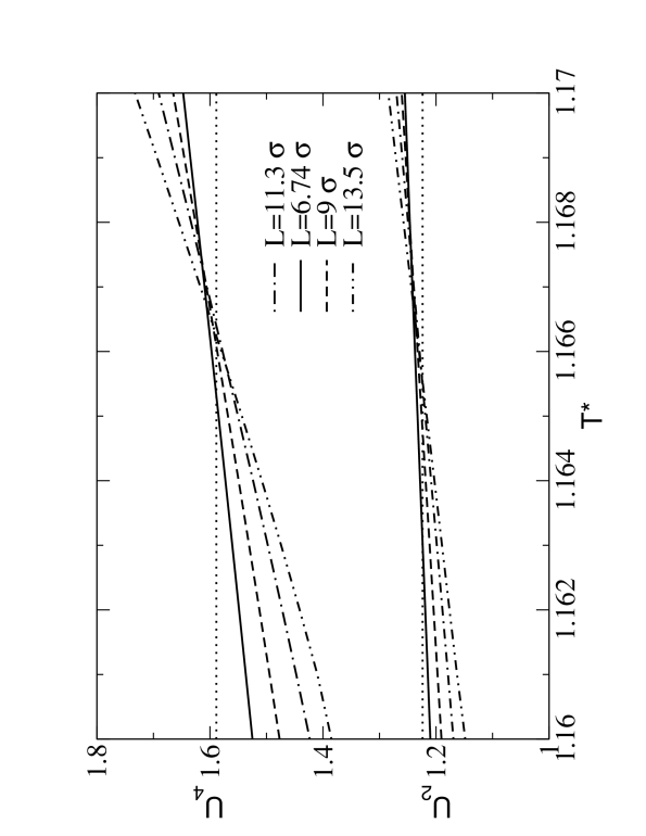
Figure 1:

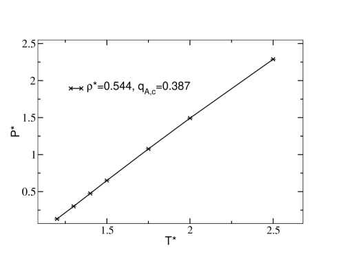
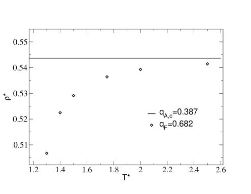
Figure 2:

Figure 3:

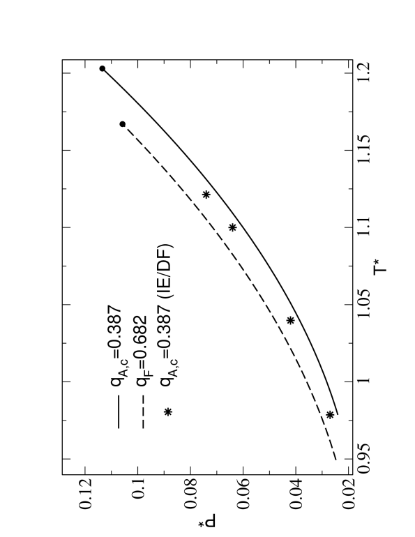
Figure 4:

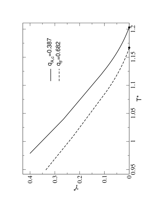
Figure 5:

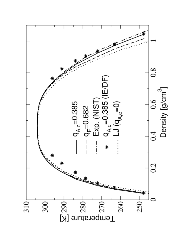
Figure 6:

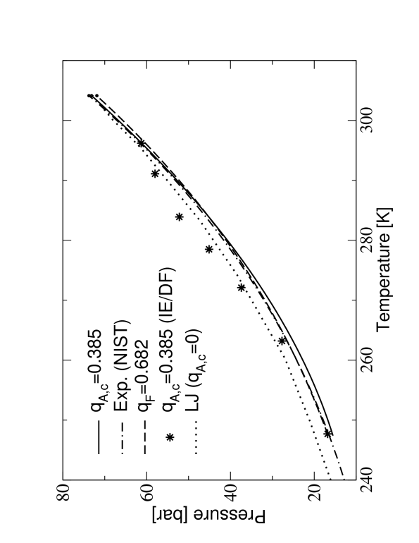
Figure 7:

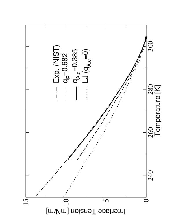
Figure 8:

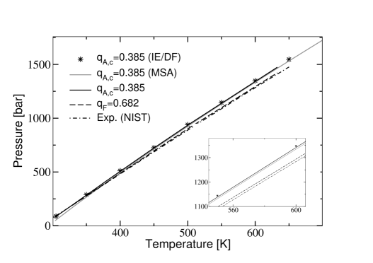
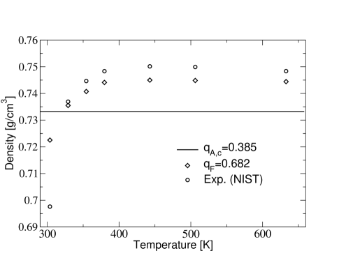
Figure 9:

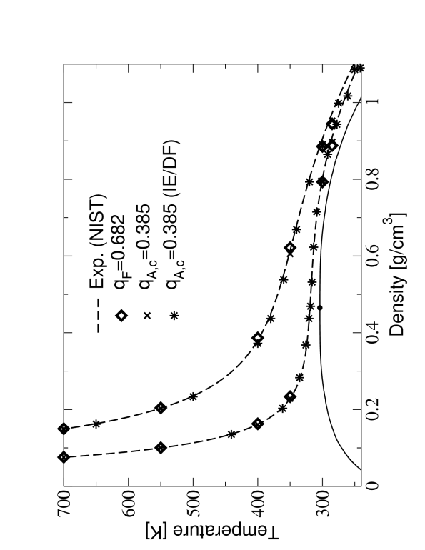
Figure 10:

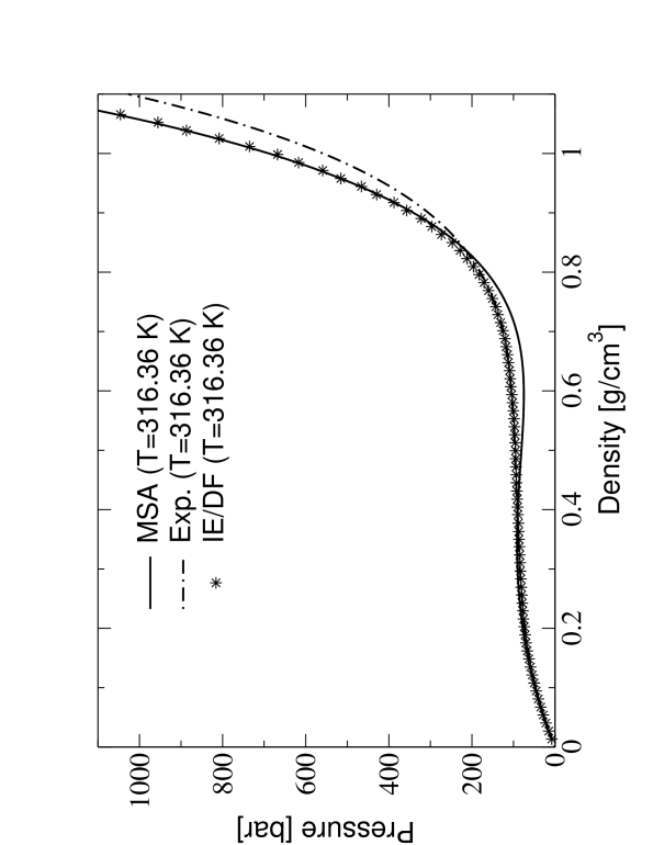
Figure 11:

References

- (1) M. P. Allen and D. J. Tildesley, Computer Simulation of Liquids (Clarendon Press, Oxford, 1987).
- (2) D. Frenkel and B. Smit, Understanding Molecular Simulation: From Algorithms to Applications, 2nd ed. (Academic Press, San Diego, 2002).
- (3) A. Z. Panagiotopoulos, Mol. Phys. 61, 813 (1987); Mol. Sim. 9, 1 (1992).
- (4) N. B. Wilding, J. Phys.: Condens. Matter 9, 585 (1997).
- (5) K. Binder, M. Müller, P. Virnau, and L. G. MacDowell, Adv. Polym. Sci. 173, 1 (2005).
- (6) E. Kiran and J. M. H. Levelt-Sengers (eds) Supercritical Fluids (Kluwer, Dordrecht, 1994).
- (7) J. J. McKetta (ed) Encyclopaedia of Chemical Processes and Design (Marcel Dekker, New York, 1996).
- (8) M. F. Kemmere and Th. Meyer (eds.) Supercritical Carbon Dioxide in Polymer Reaction Engineering (Wiley-VCH, Weinheim, 2005).
- (9) I. M. Prausnitz, R. N. Lichtenthaler, and E. G. de Azevedo, Molecular Thermodynamics of Fluid Phase Equilibria, 2nd ed. (Prentice Hall, Englewood Cliffs, 1986).
- (10) J. S. Rowlinson and F. L. Swinton, Liquids and Liquid Mixtures (Butterworths, London, 1982).
- (11) K. Binder and G. Ciccotti, Monte Carlo and Molecular Dynamics of Condensed Matter (Societa Italiana di Fisica, Bologna, 1996).
- (12) S. Bock, E. Bich and E. Vogel, Chem. Phys. 257, 147 (2000).
- (13) R. Bukowsky, J. Sadlej, B. Jeziorski, P. Jankovski, K. Szalewicz, A. Kucharski, H. L. Williams and B. M. Rice, J. Chem. Phys. 110, 3785 (1999).
- (14) C. S. Murthy, S. Singer and I. R. McDonald, Mol. Phys. 44, 135 (1981).
- (15) G. C. Maitland, M. Rigby, E. B. Smith, and W. A. Wakeham, Intermolecular forces, their origin and determination (Clarendon Press, Oxford, 1981).
- (16) H. J. Böhm, C. Meissner, and R. Ahlrichs, Mol. Phys. 53, 651 (1984).
- (17) H. J. Böhm and R. Ahlrichs, Mol. Phys. 55, 445 (1985).
- (18) S. B. Zhu and G. W. Robinson, Comp. Phys, Commun. 52, 317 (1989).
- (19) R. D. Etters and B. Kuchta, J. Phys. Chem. 90, 4537 (1989).
- (20) L. C. Geiger, B. M. Ladanyi and M. E. Clapin, J. Chem. Phys. 93, 4533 (1990).
- (21) B. J. Palmer and B. C. Garrett, J. Chem. Phys. 98, 4047 (1993).
- (22) J. G. Harris and K. H. Yung, J. Phys. Chem. 99, 12021 (1995).
- (23) J. Vorholz, V. I. Harismiadis, B. Rumpf, A. Z. Panagiotopoulos and G. Maurer, Fluid Phase Equilib. 170, 203 (2000).
- (24) J. Stoll, J. Vrabec, H. Hasse and J. Fischer, Fluid Phase Equilib. 179, 339 (2001).
- (25) J. Vrabec, J. Stoll and H. Hasse, J. Phys. Chem. B 105, 12126 (2001).
- (26) Z. Zhang and Z. Duan, J. Chem. Phys. 122, 214507 (2005).
- (27) B. M. Mognetti, L. Yelash, P. Virnau, W. Paul, K. Binder, M. Müller, and L. G. MacDowell, J. Chem. Phys. 128, 104501 (2008).
- (28) P. Virnau, M. Müller, L. G. MacDowell and K. Binder, J. Chem. Phys. 121, 2169 (2004).
- (29) E. A. Müller and L. D. Gelb, Ind. Eng. Chem. Res. 42, 4123 (2003); S. Albo and E. A. Müller, J. Phys. Chem. B 107, 1672 (2003).
- (30) G. Stell, J. C. Rasaiah and H. Narang, Mol. Phys. 27, 1393 (1974)
- (31) P. Virnau and M. Müller, J. Chem. Phys. 120, 10925 (2004).
- (32) K. Binder, Rep. Progr. Phys. 60, 487 (1997).
- (33) D. P. Landau and K. Binder, A Guide to Monte Carlo Simulations in Statistical Physics, 2nd ed. (Cambridge Univ. Press, Cambridge, 2005).
- (34) C. G. Gray and K. E. Gubbins, Theory of Molecular Fluids, Vol. I: Fundamentals. Clarendon Press Oxford (1984).
- (35) NIST website: http://webbook.nist.gov/chemistry/
- (36) K. Binder and D. P. Landau, Phys. Rev. B30, 1477 (1984); C. Borgs and R. Kotecky, J. Stat. Phys. 60, 79 (1990).
- (37) A. M. Ferrenberg and R. H. Swendsen, Phys. Rev. Lett. 61, 2635 (1988).
- (38) M. E. Fisher, in Critical Phenomena, ed. M. S. Green (Academic Press, London, 1977) p. 1.
- (39) K. Binder, Z. Physik B 43, 119 (1981).
- (40) K. Binder, in Computational Methods in Field Theory, ed. C. B. Lange and H. Gausterer (Springer, Berlin, 1992).
- (41) K. Binder and E. Luijten, Phys. Rep. 344, 179 (2001).
- (42) Y. C. Kim, M. E. Fisher, and E. Luijten, Phys. Rev. Lett. 91, 065701 (2003); Y. C. Kim and M. E. Fisher, Computer Phys. Commun. 169, 295 (2005).
- (43) J. Pérez-Pellitero, P. Ungerer, G. Orkoulas, and A. D. Mackie, J. Chem. Phys. 125, 054515 (2006).
- (44) T. Morita and K. Hiroike, Prog. Theor. Phys 23, 1003 (1960).
- (45) G. Stell, in The Equilibrium Theory of Classical Fluids edited by H. L. Frisch J. L. Lebowitz (Benjamin, New York 1964) p. II-171.
- (46) J. K. Percus, in The Equilibrium Theory of Classical Fluids edited by H. L. Frisch and J. L. Lebowitz (Benjamin, New York 1964) p. II-33.
- (47) J.–P. Hansen and I. R. McDonald, Theory of simple liquids (Academic Press, London 2006).
- (48) D. Pini and G. Stell, Physica A 306, 270 (2002).
- (49) A. Parola and L. Reatto Adv. Phys. 44, 211 (1995).
- (50) F. Lado, S. M. Foiles, and N. W. Ashcroft, Phys. Rev. A 28, 2374 (1983).
- (51) Y. Rosenfeld, J. Chem. Phys. 98, 8126 (1993).
- (52) M. Oettel, J. Phys.: Condens. Matter 17, 429 (2005).
- (53) Y. Rosenfeld, Phys. Rev. Lett. 63, 980 (1989).
- (54) R. Roth, R. Evans, A. Lang, and G. Kahl, J. Phys.: Condens. Matter 14, 12063 (2002); Y.-X. Yu and J. Wu, J. Chem. Phys. 117, 10156 (2002).
- (55) H. E. Stanley, Introduction to Phase Transitions and Critical Phenomena, Oxford University Press (Oxford 1987), chapter 7.
- (56) S. Amokrane, A. Ayadim, and J. G. Malherbe, Mol. Phys. 104, 3419 (2006).
- (57) L. G. MacDowell, M. Müller, C. Vega, and K. Binder, J. Chem. Phys. 113, 419 (2000).
- (58) L. G. MacDowell, P. Virnau, M. Müller, and K. Binder, J. Chem. Phys. 117, 6360 (2002).
- (59) R. L. C. Vink and J. Horbach, J. Phys.: Condens. Matter 16, S3807 (2004).
- (60) G. Kahl, B. Bildstein, and Y. Rosenfeld, Phys. Rev. E 54, 5391 (1996).
- (61) S. Amokrane and J. G. Malherbe, J. Phys.: Condens. Matter 13, 7199 (2001).
- (62) M. Oettel, Phys. Rev. E 69, 041404 (2004).
- (63) A. Ayadim A, J. G. Malherbe, and S. Amokrane S, J. Chem. Phys. 122, 234908 (2005).
- (64) S. Amokrane, A. Ayadim, and J. G. Malherbe, J. Phys. Chem. C 111, 15982 (2007).
- (65) A. Kostrowicka Wyczalkowska, J. V. Sengers and M. A. Anisimov, Physica A334, 482 (2004).
FIG. 1:
Second and fourth order
cumulants plotted vs. for using the
model defined by Eqs. (3,4), for four choices of
, namely and 13.5 (note that the
slope of these curves increases with ). The dotted horizontal
lines indicate the theoretical values for the 3d-Ising universality
class 40 .