Deterministic excitable media under Poisson drive: power law responses, spiral waves and dynamic range

Abstract

When each site of a spatially extended excitable medium is independently driven by a Poisson stimulus with rate $h$, the interplay between creation and annihilation of excitable waves leads to an average activity $F$. It has recently been suggested that in the low-stimulus regime ($h\sim 0$) the response function $F(h)$ of hypercubic deterministic systems behaves as a power law, $F\sim h^{m}$. Moreover, the response exponent $m$ has been predicted to depend only on the dimensionality $d$ of the lattice, $m=1/(1+d)$ [T. Ohta and T. Yoshimura, Physica D 205, 189 (2005)]. In order to test this prediction, we study the response function of excitable lattices modeled by either coupled Morris-Lecar equations or Greenberg-Hastings cellular automata. We show that the prediction is verified in our model systems for $d=1$, 2, and 3, provided that a minimum set of conditions is satisfied. Under these conditions, the dynamic range — which measures the range of stimulus intensities that can be coded by the network activity — increases with the dimensionality $d$ of the network. The power law scenario breaks down, however, if the system can exhibit self-sustained activity (spiral waves). In this case, we recover a scenario that is common to probabilistic excitable media: as a function of the conductance coupling $G$ among the excitable elements, the dynamic range is maximized precisely at the critical value $G_{c}$ above which self-sustained activity becomes stable. We discuss the implications of these results in the context of neural coding.

I Introduction

Sensory stimuli impinge continuously onto the peripheral nervous system, where they are transduced into electrical activity of sensory neurons. Understanding how those and subsequent neurons encode and process the information of the stimulus remains a formidable challenge for neuroscience since the pioneering work of Adrian Adrian (1926), and is the subject of ongoing research (see, e.g., Ref. Bhandawat et al. (2007) for recent progress on olfaction).

One of the most remarkable achievements of the nervous systems of multicellular organisms is their large dynamic range, i.e., their ability to cope with stimulus intensities which vary by many orders of magnitude. Experimental evidence in this direction is abundant, the simplest example being the century-old psychophysical laws: the psychological perception $F$ of a given stimulus intensity $h$ has been shown to be a power law for weak stimuli, $F\sim h^{m}$. This behavior of the response curve $F(h)$ is known as Stevens’ law, and the response exponent $m$ is called Stevens’ exponent in the psychophysical literature Stevens (1975). Microscopic (i.e., neural) data also confirm this scenario: the activity of relay stages in sensory processing also increases as a power law of the stimulus intensities (e.g. glomeruli and mitral cells for olfaction Friedrich and Korsching (1997); Wachowiak and Cohen (2001), or ganglion cells of the retina Deans et al. (2002); Furtado and Copelli (2006)). In both cases (psychophysical and neural), the response exponents are typically less than $1$, which indicates (as we will see below) a large dynamic range of the response curves.

That large dynamic ranges should be evolutionarily favorable is generally agreed upon, owing to the fact that natural stimuli indeed span several decades of intensity. However, experimental results show that the dynamic range of the very first sensory neurons which perform the initial transduction is usually small, their firing rate varying essentially linearly with stimulus intensity (see, e.g., Ref.Rospars et al. (2000) for the case of olfaction). Therefore, what remains to be explained is how those apparently conflicting results can be reconciled. In other words, how can large dynamic ranges be implemented by neurons?

Two main mechanisms have long been proposed. The first one is adaptation, by which neurons manage to adjust their range of operation according to the statistics of the ambient stimulus Normann and Werblin (1974); Werblin (1974); Werblin and Copenhagen (1974); Kim and Rieke (2003); Borst et al. (2005). The second one is the intrinsic variation of firing thresholds among a population of sensory neurons, which would allow them to cover a wide range of stimuli (in spite of each of them having a small range) Cleland and Linster (1999). Both mechanisms can indeed contribute to an enhancement of dynamic range. However, note that neither adaptation nor threshold variation requires interactions among neurons to work, insofar as adaptation has been understood as a dynamical process which neurons undergo individually and the firing threshold of a sensory neuron in principle does not depend on the activity of other sensory neurons. Therefore, if these were the only mechanisms responsible for enhancement of sensitivity and dynamic range, there should be no significant change in those properties if lateral connections among neurons were blocked.

Experimental data, however, suggest otherwise. Deans et al. Deans et al. (2002) have measured the response function (firing rate vs light intensity) of retinal ganglion cells of mice. For wild-type mice, they found a class of cells that responded with large dynamic range. When the same experiment was repeated with connexin36 knockout mice (i.e., mice that lack electrical synapses), they found that both sensitivity and dynamic range were significantly reduced. This suggests a third mechanism for dynamic range enhancement, based on the interaction among neurons.

This third mechanism is the subject of the present contribution. Previous work has revealed that, when excitable neurons are coupled (via chemical or electrical synapses), the response function of the resulting excitable medium indeed has much enhanced sensitivity and dynamic range Copelli et al. (2002, 2005); Copelli and Kinouchi (2005); Kinouchi and Copelli (2006); Furtado and Copelli (2006); Copelli and Campos (2007); Wu et al. (2007); Assis and Copelli (2008), as compared to those of isolated neurons. The underlying mechanism relies on very general properties of excitable media: incoming stimuli generate excitable waves which will disappear (due to the nonlinearity of their dynamics) upon collision with one another and/or with the system boundaries. For weak stimuli, waves are rare and can propagate a long way before annihilation, therefore amplification is large (as compared with what would be observed for uncoupled neurons); for strong stimuli, waves contribute little to the overall network activity (since most neurons are being externally driven), therefore amplification is small. As a result, the medium as a whole has much larger sensitivity and enhanced dynamic range as compared to those of its building blocks Copelli et al. (2002, 2005); Copelli and Kinouchi (2005); Kinouchi and Copelli (2006); Furtado and Copelli (2006); Copelli and Campos (2007); Wu et al. (2007); Assis and Copelli (2008).

The above reasoning has been tested and confirmed in a variety of models. In Refs. Kinouchi and Copelli (2006); Copelli and Campos (2007); Wu et al. (2007); Assis and Copelli (2008) the coupling among excitable elements was probabilistic (say, via a transmission rate $\lambda$). In such a scenario, low-stimulus amplification as described above occurs via stochastic excitable waves, whose (finite) lifetimes are essentially proportional to $\lambda$ (for small $\lambda$). The dynamic range then initially increases with increasing $\lambda$, up to a critical value $\lambda=\lambda_{c}$, where the system undergoes a nonequilibrium phase transition. Above $\lambda_{c}$ self-sustained activity becomes stable (i.e., small fluctuations can lead to non-zero density of active sites even in the absence of external stimuli). This hinders the coding of weak stimuli (just as a whisper cannot be heard in a sound system dominated by audio feedback), a problem that only worsens if the coupling is further increased. The dynamic range then decreases above $\lambda_{c}$ and one concludes that the maximum dynamic range is obtained precisely at the phase transition Kinouchi and Copelli (2006).

Due to their probabilistic nature, the above cited systems were cast in a framework of stochastic lattice models, from which useful insights could be obtained by applying mean field approximations and relying on well-known results of the statistical physics of nonequilibrium phase transitions. For instance, the response exponent $m$ at criticality was shown to be a critical exponent Kinouchi and Copelli (2006); Copelli and Campos (2007); Wu et al. (2007); Assis and Copelli (2008) whose value has been known for over two decades Marro and Dickman (1999). This should be contrasted with the models employed in Refs. Copelli et al. (2002, 2005); Copelli and Kinouchi (2005), where the coupling among excitable elements was deterministic. In these papers, the models were such that no self-sustained activity was observed for vanishing stimulus rates. Besides, even if a transition to the self-sustained regime occurred, the standard results from statistical physics would not be easily applicable due to the deterministic nature of the excitable waves.

In this context, our aim here is to fill two gaps: first, we verify the existence of power law responses in deterministic excitable media without self-sustained activity; second, we probe the robustness of these power laws. To accomplish the first goal, we have chosen to simulate hypercubic excitable media. This allowed us to test a theoretical prediction which has recently been proposed (based on scaling arguments) for the dependence of the response exponent $m$ on the dimensionality $d$ Ohta and Yoshimura (2005). Moreover, it reveals important differences (regarding the dependence of $m$ on $d$) with systems where coupling is probabilistic (as recently studied Assis and Copelli (2008)). To accomplish the second goal, we employed the same model to show that, with a small change in its parameters, self-sustained activity can occur, thus setting limits on the validity of the theoretical prediction. As it turns out, this last result puts the deterministic and probabilistic cases in a similar state of affairs, where the dynamic range is maximized precisely at the transition to self-sustained activity.

This paper is organized as follows. In Sec. II, the two models employed are described. The response functions in the absence and presence of self-sustained activity are analyzed in Secs. III.1 and III.2, respectively. From these response functions we obtain the dynamic range, which is dealt with in Sec. IV. Our conclusions are summarized in Sec. V.

II Models

In our simulations, we make use of a lattice in which each excitable site $i$ is governed by the Morris-Lecar (ML) equations Morris and Lecar (1981); Rinzel and Ermentrout (1998)

$$C_{m}\dot{V}_{i} = -I^{ion}_{i}(V_{i},w_{i})+I^{syn}_{i}\left(V_{i},\{V_{j}\}\right)$$ (1)

$$+I^{stim}_{i}(t)\;,$$

$$\dot{w}_{i} = \phi\left[w_{\infty}(V_{i})-w_{i}\right]\cosh\left(\frac{V_{i}-10}{29}\right)\;,$$ (2)

$$I^{ion}_{i}(V_{i},w_{i}) = G_{Ca}m_{Ca}(V_{i})(V_{i}-E_{Ca})+G_{K}w_{i}(V_{i}-E_{K})$$ (3)

$$+G_{m}(V_{i}-V_{rest})\;,$$

$$m_{Ca}(V_{i}) = 0.5\left[1+\tanh\left(\frac{V_{i}+1}{15}\right)\right]\;,$$ (4)

$$w_{\infty}(V_{i}) = 0.5\left[1+\tanh\left(\frac{V_{i}-10}{14.5}\right)\right]\;,$$ (5)

where the membrane capacitance per unit area is $C_{m}=1\mu$F/cm², membrane voltages $V_{i}$ are measured in mV, current densities in $\mu$A/cm², $\phi=1/3$ ms^-1, and maximal conductances for calcium, potassium, and passive membrane leakage are respectively $G_{Ca}=1$ mS/cm², $G_{K}=2$ mS/cm², and $G_{m}=0.5$ mS/cm². The corresponding reversal potentials are $E_{Ca}=100$ mV, $E_{K}=-70$ mV, and $V_{rest}=-35$ mV. Note that the gating variable for calcium $m_{Ca}$ is assumed to be always in equilibrium, while $w$ (which gates potassium currents) obeys a first-order dynamics Rinzel and Ermentrout (1998) (both are dimensionless). All times are expressed in milliseconds.

Even though the ML equations were developed originally to describe the membrane potential of the barnacle muscle fiber, our aim here is not to model any specific biological tissue in particular, but rather to shed light on the influence of the network topology on its response properties, particularly the dynamic range. Here we study hypercubic lattices with dimensionality $d$, restricting ourselves to the simplest case of electrical coupling, for which the synaptic currents are given by Ohm’s law,

$$I^{syn}_{i}\left(V_{i},\{V_{j}\}\right)=\sum_{j}^{2d}G_{ij}\left(V_{j}-V_{i}\right)\;,$$ (6)

where $j$ runs over the first neighbors of $i$. The conductance $G_{ij}$ between sites $i$ and $j$ could account for gap junctions (e.g. as observed in axoaxonal contacts in the hippocampus Traub et al. (1999); Lewis and Rinzel (2000) or dendrodendritic contacts of mitral cells in the olfactory glomeruli Kosaka and Kosaka (2005)) or ephaptic interactions (as modeled by Bokil et al. to occur in the olfactory nerve Bokil et al. (2001)).

The external current $I^{stim}_{i}(t)$ accounts for the stimuli arriving in the network, which we model as a Poisson process. Each neuron independently receives current pulses at constant rate $h$ (measured in ms^-1). Each pulse has duration $D$ and intensity $I_{0}$ (so that for $h\gtrsim D^{-1}$ the regime of a continuous external current is approached).

To test the robustness of the results and to allow for larger system sizes, we also simulate lattices in which each excitable element is modeled by the $n$-state deterministic Greenberg-Hastings cellular automaton (GHCA) Greenberg and Hastings (1978). In this case, each site $i$ at discrete time $t$ can be in states $x_{i}(t)\in\{0,1,2,\ldots,n-1\}$, where $x=0$ and $1$ represent a quiescent (polarized) and spiking (depolarized) neuron, respectively, whereas for $2\leq x\leq n-1$ the site is refractory. The dynamical rules are cyclical: if $x_{i}(t)\geq 1$, then $x_{i}(t+1)=[x_{i}(t)+1]\mod n$, i.e., after a spike the model neuron deterministically undergoes $n-2$ refractory steps before returning to the $x=0$ quiescent state. If $x_{i}(t)=0$, then $x_{i}(t+1)=1$ if at least one of its $2d$ nearest neighbors is spiking at time $t$ or if an external stimulus arrives at site $i$ [$x_{i}(t+1)=0$ otherwise]. The Poissonian external stimulus occurs independently at each site with probability $P=1-\exp(-h\delta)$, where $\delta=1$ ms is the time step adopted in this case.

For both models, $i=1,\ldots,N$, where $N=L^{d}$ is the total number of excitable elements in a network of linear size $L$.

III Response of hypercubic excitable media

Let $F$ be the mean firing rate, defined as the total number of spikes in an interval $T_{max}$, divided by the number $N$ of neurons and by $T_{max}$. To avoid undersampling in the low-stimulus regime, we have chosen $T_{max}=\max\{\bar{n}/(hN),100~{}\mbox{ms}\}$, where $\bar{n}$ is the approximate mean number of attempts to initiate an excitable wave (we have typically employed $\bar{n}=25$). We define the response function (or transfer function) of the network to the external stimulus as $F(h)$. In the following, we make use of a uniform coupling $G_{ij}=G$ and study how the response function changes with $G$.

III.1 Power laws

Figure 1 shows the results for a one-dimensional ML lattice with $D=0.3$ ms and $I_{0}=15$ $\mu$A/cm². As $G$ increases, three regimes are observed in the response of the network. For weak coupling [left panel in Fig. 1a, triangles in Fig. 1b], synaptic currents from spiking neighbors are not strong enough to generate spikes, so each stimulus event generates one spike, and the response function increases linearly (up to saturation at $F_{max}$, which is essentially the inverse of the refractory period). Above a certain value $G_{1}^{\prime}\simeq 0.14$ mS/cm², however, the conductance is strong enough to allow the propagation of excitable waves. In this regime [middle panel in Fig. 1a, squares in Fig. 1b], which is observed up to a second transition at $G_{1}^{\prime\prime}\simeq 0.24$ mS/cm², excitable waves are created by external stimuli and annihilated by one another and by the boundaries (open boundary conditions have been employed throughout this paper). Above $G_{1}^{\prime\prime}$, current leakage to neighbors is so large that it typically prevents neurons from spiking upon the incidence of a single stimulus pulse. What we observe [right panel of Fig. 1a] is that a neuron will fire only if it is at the boundary (in which case it has fewer neighbors and consequently less leakage) or if two stimulus pulses happen to arrive nearly consecutively (in a mimicry of temporal summation). Note that in the three panels in Fig. 1a the seed of the pseudo-random-number generator is the same, so the spikes in the left panel coincide with stimulus pulses. In the right panel of Fig. 1a, however, only the stimulus pulses that happened to fall right at the borders generated waves (all other visible perturbations are subthreshold, not spikes). In this regime, inevitably poor statistics ensues, except for large stimulus rates, as reflected in the $G=0.3$ (circles) curve in Fig. 1b. Note, however, that if a spike is finally produced, propagation of an excitable wave does occur, which explains why the response in this case is larger than for $G<G_{1}^{\prime}$.

Figure 1: (Color online) (a) Membrane potentials of 100 ML neurons versus time with $h=10^{-2}$ ms^-1 for $G=0.1$ (left panel), $0.2$, (middle panel) and $0.3$ mS/cm² (right panel). The seed of the pseudo-random number-generator is the same for the three values of $G$. (b) Response function for a one-dimensional lattice of $L=1000$ ML excitable elements. Symbols (bars) represent averages (standard deviations) over 10 runs. Solid lines are power laws discussed in the text.

Figure 2: (Color online) (a) Snapshots of networks with $50\times 50$ ML neurons, with depolarized (spiking) membrane potentials coded as white. From left to right, $G=0.1$, $0.5$, and $0.9$ mS/cm², with $h=2\times 10^{-3}$ ms^-1 and $t=3.0$ ms ($3.5$ ms) for top (bottom) row. The seed of the pseudo-random-number generator is the same for the three values of $G$. (b) Response function for a network of $200\times 200$ ML excitable elements. Symbols (bars) represent averages (standard deviations) over ten runs. Solid lines are power laws discussed in the text.

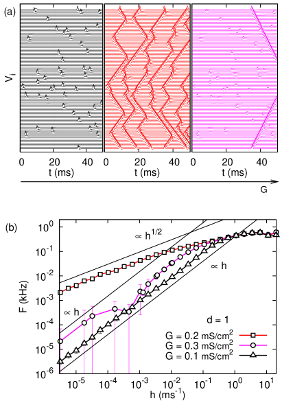
The response curves in Fig. 1b clearly show power laws $F\sim h^{m}$ in the low-stimulus regime. For $G<G_{1}^{\prime}$, the response is linear ($m=1$) and can be easily explained: for each stimulus pulse, a small number of spikes is generated (typically one) and excitable waves do not interact. For $G_{1}^{\prime}<G<G_{1}^{\prime\prime}$, however, excitable waves are created in randomly located points and annihilate upon encountering one another. To understand how this nonlinear interaction leads to a power law in the dependence of $F$ on $h$, Ohta and Yoshimura have recently proposed an elegant scaling reasoning Ohta and Yoshimura (2005). In the scaling regime, $F$ should depend on a dimensionless variable $A$. Since $h$ is small, the characteristic times for wave creation and wave annihilation are much smaller than the time of free propagation. Therefore, the only relevant parameters are the width $l$ of an excitation, the wave speed $c$, and the rate $h$. Recalling that $h$ is measured in events per unit time per site (thus having dimension of $t^{-1}L^{-d}$), we obtain $A=hc^{-1}l^{1+d}$. If we now assume a scaling relation $F\sim A^{m}$, the exponent $m$ can be obtained by noting that in the low-stimulus regime waves are sparsely distributed and the dependence of $F$ on $l$ must be linear; hence $m=1/(1+d)$ Ohta and Yoshimura (2005).

As shown in Fig. 1b, this prediction is confirmed in our one-dimensional ML simulations in the parameter region where excitable waves propagate ballistically. Particularly for $d=1$, the scaling relation $F\sim h^{1/2}$ had already been conclusively confirmed for the GHCA (in both simulations Copelli et al. (2002); Furtado and Copelli (2006) and analytical calculations Furtado and Copelli (2006)) and coupled map lattices Copelli et al. (2005). However, for more realistic models, it was only approximately verified for a chain of Hodgkin-Huxley model neurons Copelli et al. (2002) and a reaction-diffusion partial differential equation Ohta and Yoshimura (2005), with exponents around $m\simeq 0.4$. In Fig. 1b we fill this gap with an agreement over more than two decades.

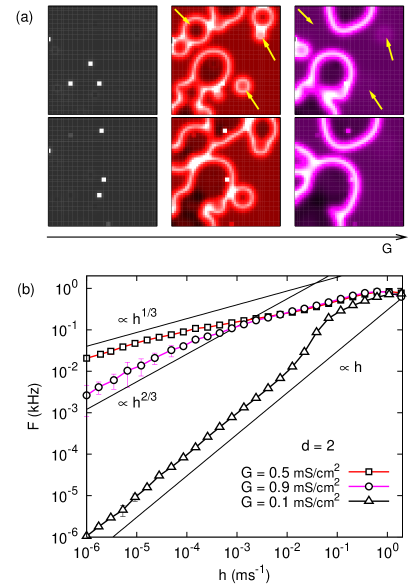
In two dimensions, simulations have been carried out with stronger stimulus pulses ($D=0.45$ ms and $I_{0}=150$ $\mu$A/cm²) to prevent excessive leakage owing to the larger number of neighbors. The same scenario has been observed. For small $G$, each stimulus pulse generates at most an evanescent wave with a radius of a few neighbors [left panel of Fig. 2a]. For $G>G_{2}^{\prime}\simeq 0.225$ mS/cm², however, generated waves can propagate ballistically with their radii increasing indefinitely. As shown in the middle panel of Fig. 2a, annihilation in this case is more complicated than for $d=1$, for now colliding waves may have different radii and their surfaces merge to form irregular-shaped excitations Lewis and Rinzel (2000); Copelli et al. (2005); Copelli and Kinouchi (2005). This regime breaks down for $G=G_{2}^{\prime\prime}\simeq 0.725$ mS/cm², above which current leakage is again too strong and spikes are generated with at least two nearly consecutive stimulus pulses or at the boundaries. Note that several waves that appear in the middle panel of Fig. 2a are absent in the right panel, as exemplified by the arrows (as in Fig. 1, the seed is the same for the three panels). Several waves in the right panel of Fig. 2a have been created at the borders (and propagate faster than those of the middle panel because $G$ is larger).

As for the response functions, Fig. 2b shows that Ohta and Yoshimura’s exponent $m=1/3$ for $d=2$ agrees (for two decades) with simulations for $G=0.5$ mS/cm² (and this holds true in the whole interval $G_{2}^{\prime}<G<G_{2}^{\prime\prime}$). Interestingly, another exponent (not predicted originally Ohta and Yoshimura (2005)) arises for $G>G_{2}^{\prime\prime}$: in this regime, waves typically require two nearly consecutive stimulus pulses to be created, and for weak stimuli this occurs approximately at a rate $h^{\prime}\sim h^{2}$. But once they are created, Ohta and Yoshimura’s reasoning is still valid, now with the dimensionless variable rewritten as $A=h^{\prime}c^{-1}l^{1+d}$. We therefore obtain the exponent $m=2/(1+d)$, which is reasonably confirmed for $G=0.9$ mS/cm² (circles) in Fig. 2b. Looking back to the analogous situation for the one-dimensional case, the circles in Fig. 1b are compatible with an exponent $m=1$ (the extremely poor statistics notwithstanding). Whether further increasing $G$ leads to other transitions (inducing the necessity of, say, $k>2$ nearly consecutive pulses to generate a wave) and new exponents [presumably $m=k/(1+d)$] is a question beyond the scope of this work, but perhaps worth pursuing. It is important to point out, however, that these transitions may have limited biological applicability: chemical synapses (which do not suffer from leakage) are not included in this model, yet abound in the nervous system.

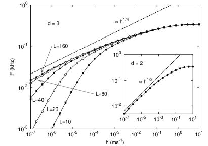
In order to test Ohta and Yoshimura’s prediction in three dimensions, we have performed simulations of the GHCA model. With the rules defined in Sec. II, an incoming stimulus pulse generates an excitable wave which propagates ballistically until annihilation with another wave or with the system borders Traub et al. (1999); Lewis and Rinzel (2000); Copelli and Kinouchi (2005), precisely as observed in the intermediate region $G^{\prime}<G<G^{\prime\prime}$ for the ML equations. The motivation for switching to a simpler model is that it allowed us to simulate much larger networks than would be feasible with the ML equations. As shown in the response functions of Fig. 3, finite-size effects are strong. However, for a network of $N=160^{3}$ automata (a system size beyond our computational resources for the ML equations), it is already possible to verify the power law $F\sim h^{1/4}$ for more than two decades. Incidentally, we note that the response function of two-dimensional GHCA networks has been studied in Ref. Copelli and Kinouchi (2005), but the power law has been missed. The inset of Fig. 3 confirms the predicted exponent.

Figure 3: Response curves of the GHCA model in $d=3$ for increasing system size ($n=3$). Inset: GHCA response function for $d=2$ ($L=2744$, averages over five runs). Dashed lines shows the response exponent $m=1/(1+d)$ for both cases.

III.2 Spiral waves

Figure 4: (Color online) Spiral waves with $\phi=0.4$ ms^-1. (a) Snapshots of networks with $50\times 50$ ML neurons, with depolarized (spiking) membrane potentials coded as white. From left to right, $G=0.15$, $0.25$, and $0.35$ mS/cm², with $h=4\times 10^{-3}$ ms^-1 and $t=20$ ms ($21$ ms) for top (bottom) row. The seed of the pseudo-random-number generator is the same for the three values of $G$. (b) Response function for a network of $200\times 200$ ML excitable elements. Symbols represent averages over five runs (standard deviations are smaller than symbol size). Firing rates were measured over 150 ms after a 50 ms transient. Horizontal and vertical lines illustrate the relevant quantities for calculating the dynamic range $\Delta$ (see Eq. (7) and text for details).

What we have described so far suggests that the response exponent is indeed $m=1/(1+d)$ whenever the following two conditions are satisfied: (A) every quiescent neuron (i.e., not only those at the borders) spikes upon the incidence of a single stimulus pulse and (B) this spike creates a deterministic excitable wave which will be annihilated at the borders or upon encountering other wave(s). In the examples shown in figures 1 and 2, these two conditions are simultaneously satisfied only for $G^{\prime}<G<G^{\prime\prime}$. For $G<G^{\prime}$, condition A is satisfied, but B is not; for $G>G^{\prime\prime}$, condition B is satisfied, but A is not.

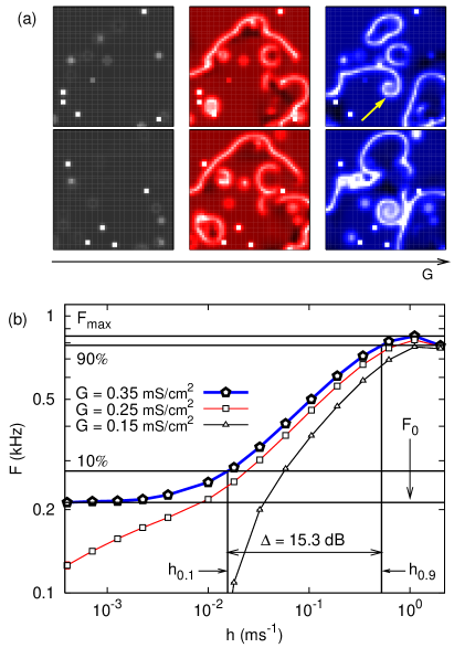
The above scenario, however, is not general. As has been known for many decades, excitable media can exhibit self-sustained activity in the form of spiral or scroll waves, a topic that has received much attention due to its relevance in different scientific branches such as cardiology Qu et al. (1999); Weiss et al. (2000), cytology Lechleiter et al. (1991), physics Merzhanov and Rumanov (1999), chemistry Winfree (1972); Petrov et al. (1997), and neuroscience Karma (1993), among others. In Fig. 2 the parameters of the ML system were such that spiral waves did not occur. With a slight deviation in parameter space, however, spiral waves may appear, even in a homogeneous lattice. As shown in the right panel of Fig. 4a, this is the case for $\phi=0.4$ ms^-1 and $G=0.35$ mS/cm² (all other parameters remaining the same), for instance. In this system, spiral waves emerge [see arrow in Fig. 4a] because of the local inhomogeneities created by the stochastic input Jung (1997) and, once established, they typically resist being destroyed by the same stochastic input (even though their shape is continuously perturbed by the Poisson pulses).

With this new phenomenon at play, how does the scenario evolve as the coupling $G$ changes? For low $G$ (say, $G<G_{2}^{\prime}$), the overall behavior of the system is the same as that of Fig. 2, i.e., a stimulus-induced spike at one site does not propagate too far [compare the left panels of Figs. 2a and  4a]. Correspondingly, the response function is linear. If $G$ is increased, a transition occurs which allows the wave radii to increase indefinitely [Fig. 2a and Fig. 4a, middle panels]. However, contrary to what was previously observed, this dynamic regime is no longer valid in a broad range of $G$ values. As $G$ is further increased, spiral waves quickly emerge. As for the second transition previously observed at $G_{2}^{\prime\prime}$, it now essentially loses meaning, for as soon as the waves are created — no matter whether by one or two incoming stimuli, or at the boundaries — the conditions are set for the spiral waves to dominate the network.

Regarding Ohta and Yoshimura’s conjecture in this scenario, the response function near the transition to self-sustained activity suffers from strong statistical fluctuations, as expected [see solid squares in the inset of Fig. 5d]. It seems compatible with a power law with exponent $m=1/3$, but for less than a decade only [note that even the self-sustained activity suffers from finite-size effects for low enough stimulus rate — see pentagons in the inset of Fig. 5d]. It is at present unclear whether larger system sizes or longer stimulus times would confirm the power law at the transition.

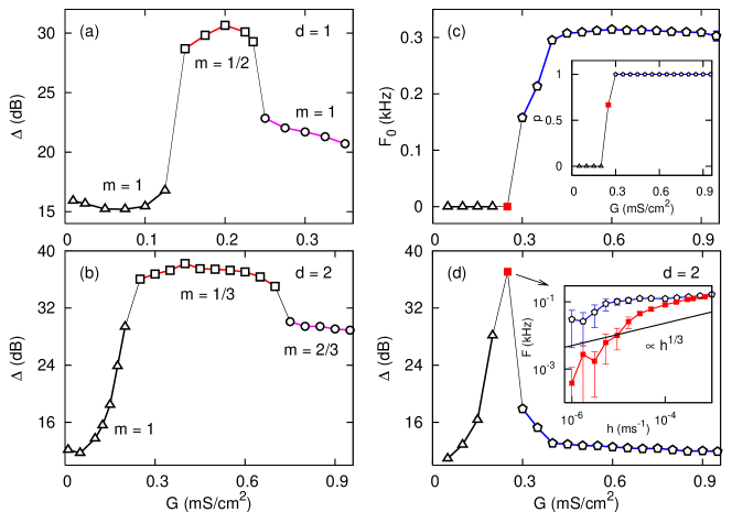
The drastic consequences of this self-sustained activity for the response curve are shown in Fig. 4b: the weak-stimulus response no longer decreases as a power law for decreasing $h$, but reaches instead a value $F_{0}$ which corresponds to the average firing rate when the lattice is dominated by spiral waves. To obtain a reasonable estimate of $F_{0}$, we simulated the following protocol: $150\times 150$ networks were stimulated during a period $T_{stim}=100$ ms with a constant rate $h=4\times 10^{-3}$ ms^-1. The stimulus was then switched off ($h=0$) and the mean activity of the network $F_{0}$ was measured after a transient $T_{trans}=900$ ms. Figure 5c shows how $F_{0}$ depends on $G$. A transition is clearly seen near $G\simeq 0.275$ mS/cm², above (below) which $F_{0}\geq 0$ ($F_{0}=0$). In the inset of Figure 5c we also show the probability $p$ that spiral waves survive after the transient, which was estimated by dividing the number of runs in which spiral waves survived by the total number of runs. The sharpness of the $p(G)$ curve also suggests a transition to a regime where self-sustained activity is stable.

This second scenario appears to be more general than the one described in Sec. III.1. We have simulated networks in which each element was modeled by the Hodgkin-Huxley equations Hodgkin and Huxley (1952) with standard parameters Koch (1999) and have obtained spiral waves. Moreover, one of the most studied causes of spiral wave creation is disorder and noise in the excitable dynamics Jung et al. (1998); García-Ojalvo and Schimansky-Geier (1999); Lindner et al. (2004), which are absent from the present study. We have nonetheless tested some ML networks where $\phi$ was distributed around $1/3$ ms^-1 with some variance, and have again obtained spiral waves. It is important to remark that, for the purposes of the present study, it is not enough that an excitable medium be able to sustain spiral waves in the absence of stimulus, say, for a given initial condition. The question is whether the Poisson stimulus is able to create spiral waves and, at the same time, allow them to survive. Consider, for instance, the limit of very weak stimuli ($h\to 0$). In this regime spiral waves hardly emerge (even for $\phi=0.4$ ms^-1) because fluctuations are not sufficiently strong [see, e.g., the open pentagons in the inset of Fig. 5d]. At the other extreme, a large value of $h$ can easily provide the necessary fluctuations, but then the created spiral waves will be statistically overshadowed by the very stimuli that generated them. Overall, the probability of self-sustained activity coexisting with the Poisson stimulus depends not only on the model parameters (in this case, $\phi$ or $G$) but also on the system size ($N$), stimulus rate ($h$), and duration ($T_{max}$). A more detailed study of this dependence would be welcome.

IV Dynamic range

Figure 5: (Color online) Left (right) column: absence (emergence) of spiral waves. Dynamic range versus coupling conductance for $\phi=1/3$ ms^-1 [(a) and (b)] and $\phi=0.4$ ms^-1 (d). Triangles denote $G<G^{\prime}$ and squares denote $G^{\prime}<G<G^{\prime\prime}$. Circles denote $G>G^{\prime\prime}$ in the absence of self-sustained activity (b), whereas pentagons denote the spiral wave regime (d). In (c), the self-sustained activity $F_{0}$ in the absence of stimulus is plotted against $G$ for fixed $\phi=0.4$ ms^-1. Inset of (c): estimated probability $p$ of spiral wave survival versus $G$ (see text for details). Inset of (d): response functions with $\phi=0.4$ ms^-1 for $G=0.25$ (solid squares) and $0.275$ mS/cm² (open pentagons). System sizes are $L=1000$ in (a); $N=200^{2}$ in (b) and (d); and $N=150^{2}$ in (c).

We can now return to the quantity that originally motivated this study. The dynamic range $\Delta$ of a response curve $F(h)$ is formally defined as Firestein et al. (1993)

$$\Delta=10\log_{10}\left(\frac{h_{0.9}}{h_{0.1}}\right)\;,$$ (7)

where $h_{0.1}$ ($h_{0.9}$) is the stimulus intensity such that the difference $F-F_{0}$ is $10$ % ($90$ %) percent of the response interval $F_{max}-F_{0}$. As depicted in Fig. 4b, $\Delta$ measures (in decibels) the range of stimulus intensities that can be “appropriately” coded by the mean firing rate of the system, discarding intensities whose corresponding responses are too close either to saturation ($h>h_{0.9}$) or to baseline ($h<h_{0.1}$). This measure of appropriateness is evidently arbitrary, but standard in the biological literature and very useful, since it is a dimensionless quantity that allows direct comparison with experimental results.

Figure 5 shows the behavior of the dynamic range (estimated numerically from the response curves) as a function of the coupling conductance. For $d=1$ [Fig. 5a], $\Delta$ changes very little for $G<G_{1}^{\prime}$, staying in the range of $16$ dB (which is comparable to experimental values of isolated olfactory sensory neurons Rospars et al. (2000) and retinal ganglion cells of connexin36 knockout mice Deans et al. (2002); Furtado and Copelli (2006)). The transition near $G_{1}^{\prime}$ seems abrupt, after which the dynamic range becomes substantially larger: the system attains $\sim 31$ dB, an enhancement of about $100$ % which had also been previously obtained with a cellular automaton model Furtado and Copelli (2006). This enhancement is clearly due to a change in the response exponent $m$, which greatly amplifies weak stimuli [recall the squares in Fig. 1b]. For $G>G_{1}^{\prime\prime}$ the dynamic range is reduced, once more because of the change in the weak-stimulus sensitivity [recall the circles in Fig. 1b]. It is important to remark that the poor statistics in Fig. 1b do not compromise the accuracy of the measured dynamic range, since the strong fluctuations occur below the sensitivity threshold $h_{0.1}$.

For $\phi=1/3$ ms^-1, the results in $d=2$ are similar [see Fig. 5b]. As $G_{2}^{\prime}$ is approached from below, the transition is somewhat smoother than for $d=1$. More importantly, since the response exponent for $G_{2}^{\prime}<G<G_{2}^{\prime\prime}$ ($m=1/3$) is smaller than for the corresponding regime in $d=1$ ($m=1/2$), the weak-stimulus amplification for $d=2$ is larger and so is the dynamic range, which reaches $\sim 38$ dB. The same trend in the dependence of $\Delta$ on $d$ is observed in the GHCA model: with a fixed system size $N=14^{6}$, by varying the dimensionality, we obtain $\Delta=31$, $43$ and $54$ dB for $d=1$, 2, and 3, respectively. Note that these values are comparable to those obtained in the ML model (the differences in $d=2$ being explained by finite-size effects, as extensively discussed in Ref. Copelli and Kinouchi (2005)).

This picture changes qualitatively when spiral waves come into play ($\phi=0.4$ ms^-1, rightmost column of Fig. 5). For $G<G_{2}^{\prime}$ the dynamic range increases monotonically with $G$, reaching a maximum near $G_{2}^{\prime}$. Increasing $G$ further, however, leads to the onset of spiral waves, and the nonzero baseline activity $F_{0}$ prevents the appropriate coding of weak stimuli. This is clearly seen in Fig. 4b (pentagons): an observer would have much difficulty in distinguishing the responses of any two points below $h=10^{-3}$ ms^-1, which leads to a drastic decrease in dynamic range. Moreover this problem becomes more and more severe as $G$ is further increased: since $F_{0}$ increases with $G$ for $G>G_{2}^{\prime}$ [see Fig. 5c], the dynamic range decreases with increasing $G$. Therefore, if a deterministic excitable medium supports spiral waves in some parameter region, its dynamic range will be maximum precisely at the transition where they become stable.

V Concluding remarks

We have simulated hypercubic networks of excitable elements modeled by the Morris-Lecar equations and Greenberg-Hasting cellular automata. We have studied how the collective response $F$ of the network to a Poisson stimulus with rate $h$ changes with the coupling $G$ and the dimensionality $d$. Two scenarios have been observed. In the first one, a broad range of $G$ values exists such that excitable waves are created and thereafter propagate ballistically, being annihilated upon encountering one another or the system boundaries. In this regime, the response function $F(h;d)$ is shown to be a power law $F\sim h^{m}$. Furthermore, we have confirmed that, if waves are created upon the incidence of a single stimulus pulse, the response exponent agrees with the theoretical prediction of Ohta and Yoshimura, $m=1/(1+d)$ Ohta and Yoshimura (2005). We have argued that in a regime where wave creation requires the incidence of two nearly consecutive stimuli, an exponent $m=2/(1+d)$ should be expected and is confirmed by our ML simulations in $d=2$ (also for a broad range of $G$ values).

If a system is such that the exponent $m=1/(1+d)$ holds, the dynamic range increases with the dimensionality $d$ (as confirmed here for $d=1$ and 2 in the ML model and $d=1$, 2, and 3 for the GHCA model). This is in stark contrast with probabilistic excitable systems, where the maximum dynamic range attained at a given dimension $d$ is a decreasing function of $d$. This happens because in that case $m$ corresponds to the critical exponent $\delta_{h}^{-1}$ (apparently belonging to the directed percolation universality class Assis and Copelli (2008)), and $\delta_{h}^{-1}$ increases with $d$.

In this context, one should not be misled by the apparent paradox posed by the assumption that a deterministic system is “just” a particular case of a probabilistic one. Consider, for instance, a probabilistic version of the $d$-dimensional GHCA in which a stimulus would be transmitted to its quiescent neighbors with probability $q$: the function $\Delta(q)$ has qualitatively the same shape as that of Fig. 5d and the maximum value of $\Delta$ attained at given $d$ is a decreasing function of $d$ Assis and Copelli (2008). Why then for $q=1$ do we have an increasing $\Delta(d)$? Remember that the main condition for the exponent $m=1/(1+d)$ to hold is the absence of self-sustained activity. In a probabilistic system, this requires not only that $q$ is precisely $1$, but also that the initial conditions are appropriately set Copelli and Kinouchi (2005); Lewis and Rinzel (2000). For $q$ infinitesimally smaller than $1$ or $q=1$ with random initial conditions, self-sustained activity ensues in the probabilistic GHCA. Therefore, in this particular model the result $m=1/(1+d)$ is obtained only under very artificial circumstances, at the edge of the parameter space and only for restricted initial conditions. In contrast, for the deterministic ML lattices studied here, the exponent holds in a broad region of the parameter space for any initial condition.

A substantially different scenario has been obtained with a change in a single parameter of the ML model, for which stable spiral waves were observed when the coupling was increased above a certain critical value (leading to a breakdown of Ohta and Yoshimura’s prediction). Given the ubiquity of spiral waves in studies of excitable media, this scenario is likely to be more general than the one previously described. In this case, a unifying picture emerges for both deterministic and probabilistic excitable media: the dynamic range in both cases is maximized at the critical value of coupling above which self-sustained activity becomes stable.

Put into a broader context, our results reinforce the idea that optimal information processing near criticality, a topic which has received much attention in recent decades Bak (1997), could have a bearing on the brain sciences. In fact, experimental results that are consistent with the hypothesis of neurons collectively operating near a critical regime have recently appeared Beggs and Plenz (2003, 2004); Eguíluz et al. (2005); Plenz and Thiagarajan (2007), joined by theoretical efforts aimed at understanding the computations themselves Bak and Chialvo (2001); Bertschinger and Natschläger (2004); Haldeman and Beggs (2005); Kinouchi and Copelli (2006) as well as the homeostatic mechanisms that could maintain the system at criticality de Arcangelis et al. (2006); Levina et al. (2007). These issues still pose remarkable challenges for the years to come, which opens the possibility of new lines of research connecting physicists with systems biology in general, and neuroscience in particular.