Density-density functionals and effective potentials in many-body electronic structure calculations

Abstract

We demonstrate the existence of different density-density functionals designed to retain selected properties of the many-body ground state in a non-interacting solution starting from the standard density functional theory ground state. We focus on diffusion quantum Monte Carlo applications that require trial wave functions with optimal Fermion nodes. The theory is extensible and can be used to understand current practices in several electronic structure methods within a generalized density functional framework. The theory justifies and stimulates the search of optimal empirical density functionals and effective potentials for accurate calculations of the properties of real materials, but also cautions on the limits of their applicability. The concepts are tested and validated with a near-analytic model.

I Introduction

Density Functional Theory (DFT) hohenberg ; kohn is based on the Hohenberg-Kohn proof of a functional correspondence between the ground state energy and the ground state density $E[\rho(r)]$. In the formulation of Kohn and Sham (K-S),kohn the interacting electron gas is replaced by non-interacting electrons moving in an effective potential. In this construction, the non-interacting density $\bar{\rho}(r)$ is equal to the interacting one $\rho(r)$ but no other property of the interacting ground state is in principle retained in the non-interacting wave function. Initially DFT was formulated to describe the total ground state energy of an interacting system and $\rho(r)$.hohenberg ; kohn ; practice Although progress towards more accurate density functionals is ongoing, current approximations such as the local density approximation (LDA)kohn ; perdew81 and more recent gradient-based extensionsRMMartinBook are already successful in predicting many electronic properties of real materials. This success has led to the use of DFT beyond its formal scope and unfortunately tempted some to believe that if we had the exact ground state density functional, we would only need to solve non-interacting problems even for properties not related to the ground state energy and density. While the virtues and limitations of the Kohn-Sham eigenvalues are discussed in textbooks,RMMartinBook ; parr the possible reasons for the success or failure of Kohn-Sham wave-functions in many-body problems are little understood and widely dispersed throughout the literature.

It is often assumed, without a formal proof, that the Kohn-Sham non-interacting ground state wave-function forms a good description of the interacting ground state wave-function to be used as the foundation of theories that go beyond DFT such as GW-Bethe Salpeter Equation (GW-BSE), Quantum Monte Carlo (QMC), or even configuration interaction (CI). This leads to an apparent contradiction in the literature since density functionals that provide wave-functions that are a good starting points in one field (as judged by comparison with experiment) are found inadequate in others. Broadly summarizing: for structural properties gradient corrected density functionalsPBE are nowadays preferred over LDA.kohn ; perdew81 Structural properties depend essentially of atomic forces which in turn are related to the density. However, for GW-BSE calculations of optical properties, an LDA-based ground state is preferredaulbur00 . In this approach a good initial approximation for the Green function is required. In QMC calculations a (non-interacting) Hartree-Fock (HF) ground state might be preferred over LDA, but the subject is still under debate. In CI calculations, instead, it is empirically claimed that the convergence with natural orbitalslowdin55 is more rapid than HF orbitals.

In Diffusion Quantum Monte Carlo (DMC) a trial wave function enforces the antisymmetry of the electronic many-body wave functionanderson79 and the nodal structure of the solution. The accuracy of the trial wave-function is critical and determines the success or failure of the method to accurately predict properties of real materials. The trial wave-function is usually a product of a Slater determinant $\Phi_{T}({\bf R})$ and a Jastrow factor $e^{J}({\bf R})$. $\Phi_{T}({\bf R})$ is often constructed with single particle Kohn-Sham orbitals or from other mean field approaches such as HF. The Jastrow, in turn, is a symmetric factor which does not change the nodes, but accelerates convergence and improves the algorithm’s numerical stability. The DMC algorithm finds the lowest energy of the set of all wave-functions that share the nodes of $\Psi_{T}({\bf R})$. The exact ground state energy is obtained only if the exact nodes are provided. Since any change to an antisymmetric wave-function must result in a higher energy than the antisymmetric ground state, the energy obtained with arbitrary nodes is an upper bound to the exact ground state energy.anderson79 Only in small systems is it possible to improve the nodes bajdich05 ; filippi00 ; umrigar07 ; rios06 ; luchow07 or even avoid the trial wave-function approach altogetherkalos00 ; zhang91 . Consequently, a general formalism that could alleviate the nodal error in large systemsalfe04 ; reboredo05 is highly desired. Quite recently it has been shown that within the single Slater determinant approach the computational cost of the DMC algorithm can have an almost linear scaling with the number of electronswilliamson ; alfe04 ; reboredo05 ; kolorenc . It is claimed, if not formally proved, that the nodes of the many-body wave-function are not too far from those of a wave function obtained via a mean field approach. However, this might not continue to hold as electron-electron interactions become more important. To improve the accuracy of these approaches and increase the range of materials to which they can be applied it is important to examine the advantages of different mean-field wave-functions.

In this paper, we demonstrate that density-density functionals can be obtained by finding the minimum of different cost functions relating the set of non-interacting $v$-representable ground state with an interacting many-body state. The minimum of these cost functions establishes a correspondence between the non-interacting and the interacting wave-functions and their associated densities and potentials. The cost function can be designed to retain selected properties of the many-body wave function in the non-interacting one. Crucially, for DMC applications the nodes can be optimized. Under certain conditions density-density functionals exist that can lead to standard scalar-density functionals. As in the case of standard DFT, this proof does not mean that we know the expression of each functional or associated potential but it will certainly stimulate the search of methods to find or approximate them. For DMC applications it is enough to prove that an optimal mean field potential for nodes exists. In order to test the theory, we find the ground state wave function of a model interacting system. Then we obtain (i) the exact DFT effective exchange correlation potential associated with the ground state density, (ii) the potential that maximizes the projection of $\Phi_{T}({\bf R})$ with the ground state. Finally, (iii) we optimize a potential to match the nodes and find that surprisingly, for this model, the non-interacting solution in the same potential as the interacting problem is a very good approximation for the nodes while the exact non-interacting Kohn-Sham ground state is particularly poor.

This paper is organized as follows: In Section II we demonstrate the existence of an different density-density correspondences associated with cost functions. We prove the existence of this functional correspondence for the case of optimal nodes required in DMC. In Section III we solve an interacting problem up to numerical precision and find its many-body ground state wave-function. Subsequently we optimize different cost functions to retain specific properties of the ground state. Finally in Section IV we discuss the relevance of our results for many-body electronic structure and give our conclusions.

II Generalized density-density functionals

Given an interaction in a many-body system, the Hohenberg-Kohn theoremhohenberg establishes a functional correspondence between densities $\rho({\bf r})$, external potentials $V(r)[\rho({\bf r})]$ and ground state wave-functions $\Psi({\bf R})[\rho({\bf r})]$; where $[\rho({\bf r})]$ denotes a functional dependence on the ground state density, and ${\bf R}$ denotes a point in the many-body $3N$ space. Since the density changes according to the strength and functional form of the interaction, this correspondence is different for different interactions. For a fixed interaction, the subset of densities $\rho({\bf r})$ corresponding to a ground state of an interacting system under an external potential $V(r)$ are denoted as pure state $v$-representable.parr A non-interacting pure state $v$-representable density is given instead by $\bar{\rho}({\bf r})=\sum_{\nu}|\phi_{\nu}\left({\bf r}\right)|^{2}$ where $\phi_{\nu}\left({\bf r}\right)$ are the Kohn-Sham-like single particle orbitals, or eigenvectors, of the Hamiltonian:

$$\left[-\frac{1}{2}{\bf\nabla}^{2}+\bar{V}\left({\bf r}\right)\right]\phi_{\nu}\left({\bf r}\right)=\varepsilon_{\nu}\phi_{\nu}\left({\bf r}\right),$$ (1)

where $\bar{V}\left({\bf r}\right)$ is an effective single particle potential. For simplicity we denote here a density to be $v$-representable if it is both pure state non-interacting and pure state v-representable. In the following we also imply pure state when we write only $v$-representable.

Each point in the sets of $v$-representable densities is associated with two different points in the wave-functions Hilbert space. In figure 1 we schematize the subset of $v$-representable densities and the functional correspondence with the subsets of the interacting and non-interacting ground state wave-functions. Note that, in principle, the two subsets of ground state wave-functions do not necessarily overlap. In the non interacting case the wave-function is given by a Slater determinant of Kohn-Sham-like orbitals but for interacting problems this simplification is not longer possible.

The Kohn-Sham scheme for density functional theory establishes a correspondence between interacting and non-interacting wave-functions represented as line (1) in Fig 1. This Kohn-Sham correspondence between wave-functions is implicit in the Khon-Sham construction for the external effective potential.kohn Figure 1 emphasizes that the wave-functions joined by line (1), while different, give the same electronic density. In more technical terms they both belong to the same Percus-Levy partition of the Hilbert spacepercus ; levy but they are the minimum energy wave-function for different interactions. The exchange-correlation potential is by construction the difference that one has to add to the external potential in a non-interacting problem so that its ground state density is the same as the interacting one. If the energy-density functional $E[\rho({\bf r})]$ is known, the effective non-interacting potential can be obtained following the standard Kohn-Sham approach. If the ground state density $\rho({\bf r})$ is known, the same correspondence between interacting and non-interacting densities can be achieved by minimizing the following function

$$K_{\rho}=\frac{1}{2}\int{\bf dr}\left[\bar{\rho}({\bf r})-\rho({\bf r})\right]^{2}.$$ (2)

within the subset of non-interacting $v$-representable densities. Formally, this could be done by exploring all values $\bar{V}\left({\bf r}\right)$ in Eq (1).

In practice, if the density of the interacting ground state is known, the potential $\bar{V}_{K_{\rho}}({\bf r})$ that minimizes Eq. (2) can be obtained numerically with a procedure similar in spirit to the optimized effective potential (OEP) method. The change in the density required to minimize Eq. (2) is

$$\Delta_{\rho}=-[\bar{\rho}({\bf r})-\rho({\bf r})].$$ (3)

Within linear response, the change in the potential required to produce $\Delta_{\rho}$ is

$$\Delta\bar{V}_{K_{\rho}}({\bf r})=\int{\bf dr^{\prime}}\left[\rho({\bf r^{\prime}})-\bar{\rho}({\bf r^{\prime}})\right]\frac{\delta V\left({\bf r^{\prime}}\right)}{\delta\rho\left({\bf r}\right)}$$ (4)

Adding recursively $\Delta\bar{V}_{K_{\rho}}({\bf r})$ we can find the potential $\bar{V}_{K_{\rho}}({\bf r})$ associated with $K_{\rho}=0$ (see an example below).

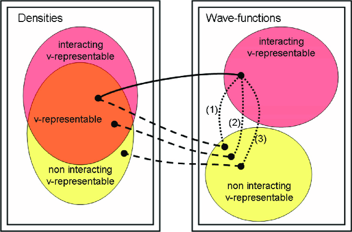
Figure 1: (Color online) a) Representation of the sets of pure state $v$-representable interacting densities. b) Sets of interacting and non-interacting ground state wave-functions. The Kohn-Sham formulation of DFT relates a $v-representable$ density with a pair interacting and a non-interacting wave-function. The same functional correspondence can be obtained minimizing Eq. (2) (line 1 in the figure). Different cost functions relate an interacting $v$-representable density with a different non-interacting-$v$ representable density (see lines 2 and 3).

II.1 Other density-density correspondences

It is often desirable o preserve properties in addition to the density of the many-body ground state $\Psi({\bf R})$ in a non-interacting wave-function $\Phi_{T}({\bf R})$ to be used as a starting point for theories that go beyond DFT. This task involves exploring all the non-interacting $v$-representable set in order to find a wave-function that best describes a given property. This is a typical optimization problem. One of the most common strategies in optimization is the design of a cost function. One example is Eq (2), a measure of the difference in two densities. Another example of a cost function is

$$K_{Det}=-\left|\left<\Psi\right.\left|\Phi_{T}\right>\right|^{2}$$ (5)

which involves a projection of the interacting ground state $\Psi$ in the set of non-interacting $v$-representable wave-functions $\{\Phi_{T}\}$. The minimum of Eq. (5) is the non-interacting ground state Slater determinant with maximum projection in the interacting ground state. We have claimed above that the interacting wave-functions might be in general very different from a single non-interacting Slater determinant. Accordingly, we expect $K_{Det}>-1$.

We expect to find a different minimum in the non-interacting ground state set, if we change the functional form of the cost function from Eq. (2) to Eq. (5) for the following reasons:

1) We can visualize the cost function as a scalar potential defined in the full Hilbert-space. Although different cost functions can share the same minimum in the complete Hilbert space, in the restricted subset of non-interacting ground state wave-functions, different cost functions can have a different minimum: the optimal point found depends on the functional form of the cost function. Accordingly, while all the cost functions we propose here would be minimized if we could reach the interacting many body state $\Psi$ ( where, of course, every property is retained exactly), because our search is constrained to non-interacting $v$-representable subset the minimum we would find will depend on the properties we wish to retain.

2) The Hohenberg Kohn theorem, when applied to the non-interacting $v$-representable case implies that, in the absence of degeneracy, there is at most one wave-function that has the same density as the interacting case. Therefore, once the minimum of an arbitrary cost function is found, its associated non-interacting density can no longer be equal to the interacting density unless the property enforced by the cost function can be related back to density. Enforcing the non-interacting density to remain equal to the interacting ground state density prevents all other properties of the non-interacting wave-function from being further improved. If we intend to optimize other properties, we have to relax the density constraint finding a different wave-function associated with a different density.

The minimization of different cost-functions, relating the interacting ground state $\Psi({\bf R})$ with the non-interacting $v$-representable set, provide in-principle different correspondences between interacting and non-interacting wave-functions represented as different lines in figure 1. Each cost function $K$ defines a correspondence different than the identity between pure state $v$-representable densities and non-interacting pure-state $v-$representable densities. As a consequence, the idealized optimization processes outlined here defines an operator $U_{K}$ that turns each $\rho({\bf r})$ into a non-interacting density corresponding to the wave-functions $\Phi_{T}({\bf R})$ which is the minimum of a cost function $K$.

$$\bar{\rho}_{K}({\bf r})=U_{K}\left[\rho({\bf r})\right].$$ (6)

Note that if the minimum of a given cost function $K$ is a single $\Phi_{T}({\bf R})$ for every $v$-representable density, then $U_{K}$ defines a density-density functional. When more than one non-interacting $v$-representable wave-function give the same optimal value for $K$, the degeneracy can be broken by additional requirements in the cost function [e.g. also minimizing Eq. (2), the difference between the current and pure state densities ]. Since we only need one optimal wave-function, any from a degenerate minimum can be chosen to construct the density-density functional $U_{K}$. When minimization of a cost function defines a one to one correspondence with an inverse, a more usual energy-density functional of the form $E\{U_{K}^{-1}[\bar{\rho}_{K}({\bf r})]\}$ can be constructed. Only a restricted class of cost functions lead to density transformations with an inverse. Minimization of the cost functions among all pure-state-non-interacting $v$-representable densities defines the optimal effective potential which is a function of this density.

Given a cost function, $K$, finding an approximation for the density transformation operator $U_{K}$ could certainly be as demanding as finding an approximation for the energy-density functional $E\left[\rho({\bf r})\right]$ required by DFT based methods. This task is beyond the goal of this paper. However, we will show that we can expect the operator associated to the best nodes for DMC ($U_{DMC}$) to be non-local and very different from the identity. Accordingly we can expect non-interacting wave-functions with good nodes to be a poor source of densities. Moreover, for the example considered below, we find, that the direction we might have to explore to optimize the potential might be surprisingly different than the attempts considered so farwagner03 ; kolorenc .

II.2 The Diffusion Monte Carlo case

We next show that optimization of the nodes for DMC among the set of $v-$representable wave-functions leads to a correspondence between pure state $v$-representable densities and pure state non-interacting $v$-representable densities of the class described above. These in turn demonstrate the existence of an optimal effective non-interacting nodal potential.

Since, the ground state density $\rho({\bf r})$ determines the ground state wave-function $\Psi({\bf R})[\rho({\bf r})]$,hohenberg $\rho({\bf r})$ defines also the points ${\bf R}$ of the nodal surface $S_{0}({\bf R})[\rho({\bf r})]$ where $\Psi({\bf R})[\rho({\bf r})]=0$. We can also classify the nodal surfaces in pure state v-representable and pure-state-non-interacting $v$-representable.

The DMC algorithm in the fixed node approximation finds the lowest energy of the set of all wave-functions that share the nodes or the trial wave-function. For Slater determinant Jastrow wave-functions, the nodes of the trial wave-function are by construction those of $\Phi_{T}({\bf R})$; that is they are pure-state non-interacting $v$-representable. The DMC energy, $E_{DMC}$ is also a function of the external potential which in turn is a function of the interacting ground state density $V(r)[\rho({\bf r})]$. Thus minimization of $E_{DMC}[\Phi_{T}({\bf R}),\rho({\bf r})]$ in the set of non-interacting $v$-representable wave-functions $\Phi_{T}({\bf R})$ determines one $\Phi_{T}({\bf R})$ with the best nodes. Every optimal $\Phi_{T}({\bf R})$ defines an optimal auxiliary density $\bar{\rho}_{DMC}({\bf r})$. As a consequence optimizing the nodes of the trial wave-function by perturbing the nodes of pure state non-interacting wave-functions implies finding another correspondence between interacting and non-interacting densities (another line in figure 1). The best cost function for optimal nodes is ultimately the DMC energy itself.

Since we restrict the search to pure-state non-interacting $v$-representable nodes, the minimum energy $E_{DMC}[\rho({\bf r}]$ will be larger than the true ground state energy $E[\rho({\bf r}]$, because of the upper bound theorem, unless $S_{0}({\bf R})$ is non-interacting $v$-representable.

Note that for an arbitrary interaction $S_{0}({\bf R})$ is not expected to be, in general, pure-state-not-interacting v-representable. However, if $S_{0}({\bf R})$ were non-interacting v-representable, the best Slater Determinant $\Phi_{T}({\bf R})$ for DMC could be formally found by finding the minimum of the cost function

$$K_{S_{0}}=\int_{S_{0}}{\bf dS}\left|\Phi_{T}({\bf R})\right|^{2}.$$ (7)

where $\int_{S_{0}}$ denotes a surface integral over the interacting nodal surface.

III Cost function minimization

To demonstrate the theoretical concepts above we solve a simple non-trivial interacting model as a function of the interacting potential strength and shape. We then optimize the wave-functions to minimize the cost functions in Eqs. (2), (5) and (7) so as to find the exact DFT wave-function, the wave-functions that maximize the projection on the interacting ground state and minimize the projection on the nodes. Subsequently, we estimate the volume of the Hilbert space enclosed between the nodes of the interacting wave-functions and the optimized non-interacting ones.

III.1 A model interacting ground state

For illustrative purposes we choose the interacting problem to be as simple as possible and yet not trivial. We solve the ground state of two spin-less electrons moving in a two dimensional square of side length 1 with a repulsive interaction potential of the form $V({\bf r},{\bf r^{\prime}})=8\gamma\cos{[\alpha\pi(x-x^{\prime})]}\cos{[\alpha\pi(y-y^{\prime})]}$. units While this potential is different than the Coulomb interaction, it shares some of its properties. For positive $\gamma$ and $|\alpha|<1$ the interaction is repulsive with a repulsion that increases monotonically when for shorter distances. The amplitude of the repulsion as compared to the kinetic energy can be changed by adjusting $\gamma$. Since the Coulomb interaction is self similar, changing $\gamma$ mimics what happens in a real system when we change the size of the system. The shape of the potential within the confined region can be altered by changing $\alpha$. In the limit of $\alpha\rightarrow 0$ the interaction potential is separable which allows several limits to be tested (such as the nodes). The functional form facilitates an analytical treatment of the problem by removing the singularity of the Coulomb interaction at short distances.

We expanded the many-body wave-function in a full CI on non-interacting Slater determinants with the same symmetry as the ground state. The ground state is degenerate because there are only two electrons. We chose one of the ground state wave-functions according to the $D_{2}$ subgroup of the $D_{4}$ symmetry of the Hamiltonian. With this choice, $\rho({\bf r})$ has $D_{2}$ symmetry ($x$ is not equivalent to $y$). The basis of Slater determinants was constructed with functions of the form $16\mathrm{sin}(n\pi x)\mathrm{sin}(m\pi y)$ with $n$ and $m<8$. Since parity is preserved by the interaction and Slater determinants of identical functions are zero, the size of the basis set is reduced to only 300 in our calculations.

Most of the calculations reported here were done analytically with the help of the Mathematica package, including all of the electron-electron interaction integrals.notebook The only source of errors are numerical truncation and the size of the basis, which was tested for convergence.

In Figure 2 we show the quadrants of densities corresponding to wave-functions that are even for reflections in the $y$ direction and odd in the $x$ direction for $\gamma=2$ and $\alpha=1$. Figure 2(a) shows the upper left quadrant of the density of the interacting ground state of two spin-less electrons obtained with full CI. Figure 2(b) shows the upper right quadrant of the non-interacting density corresponding to the effective potential obtained by adding recursively $\Delta V_{K_{\rho}}({\bf r})$ [Eq. (4)], which is exactly the reflection of $\rho({\bf r^{\prime}})$ Fig. 2(a) up to numerical precision [$K_{\rho}=0$ in Eq. (2)]. Because of the Hohenberg-Kohn theorem,hohenberg $V_{K_{\rho}}$ and the Kohn-Sham potential $V_{KS}(\rho)$ can only differ by a constant and thus the wave-functions coming from this potential are the exact DFT wave-functions for our interaction. The properties of the wave-functions will be discussed later in the text. The densities in Figs. 2(d) and 2(d) correspond to the minimum of the cost functions given in Eqs (5) and (7) obtained as described below.

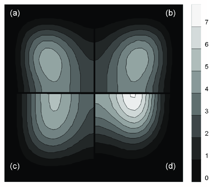
Figure 2: Ground state densities, in particles per unit area, for two interacting spin-less electrons in a square box. The complete density can be obtained by reflections (see also Fig 3). (a) Full CI ground state interacting density. (b) Exact DFT solution obtained minimizing Eq. (2). (c) Slater determinant with maximum projection with CI the ground state [see Eq. (5)]. (d) Slater determinant with minimum amplitude on the nodes of the CI ground state [see Eq. (7)].

III.2 Effective potential optimization

We now consider more difficult cost functions than density differences, Eq. (2). For non-interacting $v$-representable densities there are also functional correspondences between ground state wave-functions, potentials and densities. This concept has been exploited in the optimized effective potential (OEP) for exact exchange. xxtheory ; xxsemiconductors ; xx2deg ; us The exchange potential can be calculated in OEP xxtheory ; xxsemiconductors ; xx2deg ; us as:

$$V_{x}({\bf r})=\frac{\delta E_{x}}{\delta\rho\left({\bf r}\right)}$$ (8)

$$=\sum_{\nu}^{occ}\int\!\!\!\!\int\!\!{\bf dr^{\prime}}{\bf dr^{\prime\prime}}\left[\frac{\delta E_{x}}{\delta\phi_{\nu}\left({\bf r^{\prime\prime}}\right)}\frac{\delta\phi_{\nu}\left({\bf r^{\prime\prime}}\right)}{\delta V_{KS}\left({\bf r^{\prime}}\right)}+c.c.\right]\!\!\frac{\delta V_{KS}\left({\bf r^{\prime}}\right)}{\delta\rho\left({\bf r}\right)}.$$

In Eq. (8), the functional derivative $\delta E_{x}/\delta\phi_{\nu}\left({\bf r}\right)$ is evaluated directly from the explicit expression for the exchange energy $E_{x}$ in terms of $\phi_{\nu}\left({\bf r}\right)$. Next $\delta\phi_{\nu}\left({\bf r}\right)/\delta V_{KS}\left({\bf r^{\prime}}\right)$ is evaluated using first-order perturbation theory from Eq. (1). Finally ${\delta V_{KS}\left({\bf r^{\prime}}\right)}/{\delta\rho\left({\bf r}\right)}$ is the inverse of the linear susceptibility operator. If there are fixed boundary conditions such as the number of particles, the susceptibility operator is singular xxsemiconductors ; us . Excluding these null spaces it can be inverted numerically.xxsemiconductors We use earlier this susceptibility operator in Eq. (4). Equation (8) is by construction the gradient of the exchange energy in the set of pure-state-non-interacting $v$-representable densities. While we are not going to attempt an exact exchange approach in this paper, the ability to calculate gradients allow us to minimize cost functions as long as the cost function $K$ can be expressed in terms of non-interacting ground state wave wave-functions or eigenvalues. The potential that minimizes $K$ can be obtained by recursively applying the formula

$$\delta V_{K}({\bf r})=\epsilon\sum_{\nu}^{occ}\int\!\!{\bf dr^{\prime}}\!\!\frac{\delta K}{\delta\phi_{\nu}\left({\bf r^{\prime}}\right)}\frac{\delta\phi_{\nu}\left({\bf r^{\prime}}\right)}{\delta V_{KS}\left({\bf r}\right)}+c.c.$$ (9)

Equation (9) gives the direction we need to change the potential to minimize the cost function. The magnitude of the change is controlled by $\epsilon$, which can be adjusted as one reaches the minimum.

Replacing $K$ by $K_{Det}$ in Eq. (9) and using Eq (5) and first order perturbation theory we find

$$\delta V_{K_{Det}}({\bf r}) = \epsilon\left<\Psi\right.\left|\Phi_{T}\right>\sum_{\nu}^{o}\sum_{n}^{u}\left<\Psi\right|c^{{\dagger}}_{n}c_{\nu}\left|\Phi_{T}\right>\frac{\phi_{n}({\bf r})\phi_{nu}({\bf r})}{\varepsilon_{\nu}-\varepsilon_{n}}$$ (10)

$$+ c.c.$$

In equation (10) $\sum_{n}^{o}$ ( $\sum_{n}^{u}$ ) means sum over occupied (unoccupied) states, while $c^{{\dagger}}_{n}$ and $c_{\nu}$ are creation and destruction operators on the non-interacting ground state $\left|\Phi_{T}\right>$. One can understand also the state $c^{{\dagger}}_{n}c_{\nu}\left|\Phi_{T}\right>$ as the many body wave-function $\Phi_{T}^{n,\nu}(R)$ resulting from replacing the occupied state $\phi_{\nu}$ by the $\phi_{n}$. This is equivalent to creating an electron hole pair excitation in a non-interacting ground state. In Eq. (10) a term in the potential is added every time an electron hole pair excitation has no zero projection to the interacting ground state. Since the basis of products of wave-functions $\phi_{n}({\bf r})\phi_{\nu}({\bf r})$ is over-complete, there are linear combinations with non-zero coefficients that add up to zero. A minimum is found when the gradient of the cost function with respect to variations of the effective potential is zero. If the absolute minimum is found, the wave function can only be improved further by a multi-determinant expansion, that is, outside the set of pure-state non-interacting densities. Since we choose a basis expansion for the single particle orbitals to be sine functions, the products $\phi_{n}({\bf r})\phi_{nu}({\bf r})$ are linear combinations of sine products. These sine products can be transformed analytically to cosines. The change in the potential is thus written in a cosine basis which is complete. All coefficients must vanish in the cosine basis when a minimum is found. This allows us to verify that the gradient in the potential can be minimized up to numerical precision. The integrated effective potential is thus naturally expressed as a linear combinations of cosines, which allows the analytical calculation of the coefficients of the effective potential matrix in a basis of sines, where the kinetic energy is diagonal. The Slater determinant $|\Phi_{T}>$ is written in the same basis as the interacting ground state $|\Phi>$. The projections involved in Eq. (10) are then reduced to a scalar product of the vectors of coefficients.

In figure 2(c) we show the ground state density associated to minimization of Eq. (5) for the same parameters as the interacting ground state density in Fig 2(a). We see that while optimizing the cost function (2) allows matching the interacting density exactly, optimizing the wave-function projection requires a significant change in the resulting density.

Similarly, replacing $K$ by $K_{S_{0}}$ in Eq. (9) and using Eq (7) we get

$$\delta V_{K_{S_{0}}}({\bf r}) = \epsilon\sum_{\nu}^{o}\sum_{n}^{u}\int_{S_{0}}\;\;{\bf dS}\Phi_{T}^{n,\nu}({\bf R})\Phi_{T}({\bf R})\frac{\phi_{n}({\bf r})\phi_{nu}({\bf r})}{\varepsilon_{\nu}-\varepsilon_{n}}$$ (11)

$$+ c.c.$$

Unlike Eqs.4 and 10, a complication appears when evaluating the integral over the nodal surface $\int_{S_{0}}{\bf dS}$. This integral involves finding the points where the many-body wave-function is zero. The problem is simplified because the derivatives of the many body wave-functions can be obtained analytically. Consequently, starting from an arbitrary point ${\bf R}$ we can find a zero recursively with the Newton-Raphson method, ${\bf R}_{n+1}={\bf R}_{n}+\Psi({\bf R}){\bf\nabla}\Psi({\bf R})/\left|{\bf\nabla}\Psi({\bf R})\right|^{2}$. Next we make a random displacement ${\bf\Delta R}$ in the hyper-plane perpendicular to ${\bf\nabla}\Psi({\bf R})$ within a circle of radius 0.05 and find a node again. We repeat this process $50$ times and select an element of $\{{\bf R}\}_{S}$. With this parameters, the random position ${\bf R}_{n}$ can travel across the full size of the system so that the distribution is homogeneous. By repeating this process $N=500$ times, excluding points at the boundaries which are zero by construction, we generate an homogeneous distribution of points at the nodal surface $\{{\bf R}\}_{S}$. We approximate the integral in Eq. (7) as a sum on the values on the set $\{{\bf R}\}_{S}$. Note that while the total area of the surface would be in general involved as a factor, the value of this area is not relevant since we are interested in finding a minimum of the cost function and the position of the minimum of any function is not altered by a positive multiplicative constant. The sum over random points introduces a relative error of order $1/\sqrt{500}$ . Replacing the integral with a summation creates also many local minima in the landscape of Eq. (11). Accordingly, we tested different initial conditions; the best results are obtained starting from $V_{K_{S_{0}}}=0$.

The density resulting from minimization of Eq. (7) is plotted in Fig 2(d). We see here again a significant change as compared with the fully interacting CI ground state [see Fig 2(a)] and the the exact DFT non-interacting solution Fig 2(b).

Figure 2 is a clear example that corroborates our claim in Section II.1 that enforcing different properties on the non-interacting wave-function implies a density-density correspondence different than the identity between the interacting and non interacting systems. Similar results are observed as function of the strength and shape of the interaction [controlled by $\gamma$ and $\alpha$]

A comparison between Eqs. (10) and (11) clearly shows that the relative values of the coefficient multiplying $\phi_{n}({\bf r})\phi_{nu}({\bf r})$ depends fundamentally on the cost function. Therefore, even starting from the same effective potential and $\Phi_{T}({\bf R})$ the coefficient affecting each individual product $\phi_{n}({\bf r})\phi_{nu}({\bf r})$ depends on the functional form of the cost function. This change in the potential remains present when the potential is written in the complete cosine basis. Thus, the effective potential must change in accord with the property of the interacting ground state that one aims to enforce in the non-interacting ground state with a cost function.

Figure 3 shows the effective potentials used for the calculations shown in Fig 2. We show in Fig 3(a) a constant, since in the interacting problem solved with full CI no effective external potential was added. Figures 3(b) [minimum of Eq. (2)], 3(c) [minimum of Eq. (5)] and 3(d) [minimum of Eq. (7)] show a clear change in the effective potential depending on the cost functions. As argued earlier Fig. 3(b) shows the exact Kohn-Sham DFT potential for this interaction which implies that a different density functional must be used to obtain non-interacting wave-functions preserving properties other than the density.

Note that Eq. (7) could be zero only for a pure-state-non-interacting $v$-representable nodal surface. However, if the nodes are not, replacing in $K_{S_{0}}$ could result in a potential that simply prevents the non-interacting wave-function to reach regions of space where the nodes are more troublesome. The potential shown in Fig. 3(d) presents a maximum in regions where instead Figs. 3(b) and 3(c) develop a minimum. These are the regions where the electrons in the many-body wave-functions tend to localize because of correlation effects. The maximum in Fig 3(d) suggest the possibility of non-$v$ representability by a non-interacting wave-function in this model.

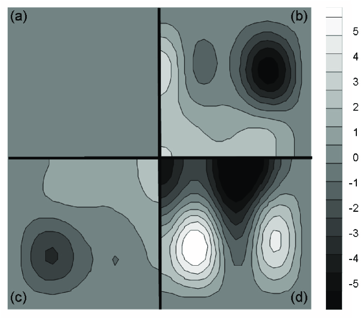
Figure 3: Optimized effective potentials corresponding to the densities in Fig. 2. The complete potentials can be obtained by reflection on the black lines. Gray level valuesunits are given on the right. The optimal effective potentials are strongly dependent on the property we target to retain in the wave-function.

III.3 Wave-function internal structure

In order to quantitatively test the quality of the nodes of the wave-functions found by minimization of Eqs. (2), (5) and (7) and to test the convergence of the nodes of the full CI calculations, we take advantage of the homogeneous distribution of points $\{{\bf R}\}_{S}$ at the nodal surface $S_{0}({\bf R})$ described earlier.

For each point ${\bf R}$ in $\{{\bf R}\}_{S}$ we can find the distance $\ell_{i}$ to the node of another wave-function $\Phi_{T}({\bf R})$ in the direction of ${\bf\nabla}\Psi({\bf R})$. Thus

$$\Delta V=\frac{1}{N}\sum_{i}\ell_{i}$$ (12)

is an approximated measure of the fraction of the Hilbert space volume between the nodal surface of $\Phi_{T}({\bf R})$ and $\Psi({\bf R})$ and

$$\delta\rho=\frac{1}{3N}\sum_{i}\ell_{i}\left|\Phi_{T}\left({\bf R}_{i}\right)\right|^{2}$$ (13)

measures the probability density inside $\Delta V$.

We can use Eqs. (12) and (13) to test the convergence of the CI ground state nodes as a function of the size of the basis set. While the ground state energy requires $40$ basis functions, the nodes are more difficult to converge requiring four times as many. The size of the basis required to converge the nodes was determined for $\gamma=2$ plotting $\delta\rho$ between the CI ground state with 300 wave-functions and the CI ground state obtained using a reduced basis.

The quantities in Eqs. (12) and (13) can be used also to characterize the nodes of different wave-functions as compared with the exact node. In figure 4 we show the volume enclosed between the nodes $\Delta V$ of different optimized $\Phi_{T}({\bf R})$ and the interacting ground state $\Psi({\bf R})$ as a function of the strength of the interaction potential $\gamma$. Note that the Kohn-Sham DFT solution gives a significantly larger volume than other optimized wave-functions. The difference increases as the interaction strength increases. The wave-function that results from minimizing Eq. (5) which targets wave-function projection fares very well over the range explored. In turn, minimization of $K_{S_{0}}$ [see Eq. (7)] results in nodes that are only sometimes marginally better. Surprisingly, the non-interacting solution, that is the non-interacting ground state in the absence of any effective potential, is remarkably good. Similar results are found by altering the shape of the potential with $\alpha$.

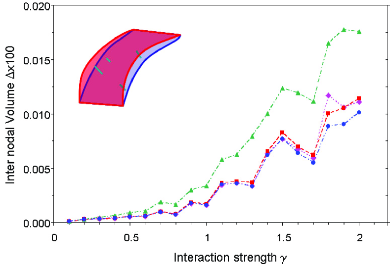
Figure 4: (Color online) Fraction of the Hilbert space $\Delta V$ between the full CI node and the nodes of different optimized wave-functions. Triangles correspond to the exact DFT wave-function [Eq. (2)], squares to maximum projection [Eq. (5)], rhombi to the minimum amplitude at the nodes [Eq. (7)] and circles to the non-interacting ground state. The inset shows the method used to estimate $\Delta V$

In figure 5 we plot the values $\delta\rho$ for different optimized wave-functions as a function of $\gamma$. We see again that the exact Kohn-Sham DFT solution is not the best. The quantity $\delta\rho$ is a measure on how much the error in the nodes would affect the probability density and thus it can be understood as the as a measure of the nodal error in the ground state energy. Again in this case the non-interacting ground state without any effective potential is the best approximation.

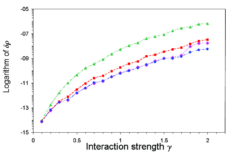
Figure 5: (Color online) Probability density inside the volume between the nodes of the full CI wave-function and optimized wave-functions. Same conventions and symbols as in Fig. 2

IV Discussion

Although the numerical investigation of the different density-density functionals described above required numerical representation of the many body ground state wave-function, the conclusions that we draw have general value. The model we explore is simplified but has the advantages that the results can be converged and are free of significant approximations. The simplified interaction used in the model retains essential features of the Coulomb interaction.

We have shown (Fig. 2 and 3) that the effective densities and potentials are explicit functions of a cost function. Potentials and densities very different to the exact DFT solutions are obtained if we enforce properties beyond $\rho({\bf r})$ in the cost function. The exact DFT wave-function matches $\rho({\bf r})$ with complete disregard to other elements of the many body wave-function structure. Since the Hohenberg-Kohn theoremhohenberg is valid, optimizing other properties of the non-interacting ground state in general requires changing the potential with a resulting impact on the density.

We find that mean field methods, while giving an accurate description of the density can mislead us in other aspects of the wave-function structure such as the nodal surface. In this paper we argue that, among the pure-state-non-interacting $v$-representable densities, there is at least one that more accurately describes the interacting ground state nodes. We can optimize the wave-function associated with this density with a cost function. The cost function form depends on the property we target to retain and also the optimal density we find. For the nodes, the optimal cost function is clearly the DMC energy. A fixed cost function establishes a density-density correspondence which can be described as an operator $U$ that transforms interacting densities into non-interacting ones.

While finding the functional form of $U_{DMC}$ is a task beyond the scope of this paper, we argue that we can expect this operator to be highly non-local and very different from the identity, in particular for strong electron-electron correlations. We find that we can improve the nodes with some simple cost functions, but the best nodes we found were obtained solving the non-interacting problem without the addition of any effective potential. We cannot exclude the possibility that this result might well be an accident of the model. Our result, however, shows that the popular expectation that the DFT solution is a good starting point for nodes is not valid in general.

Optimal wave-functions can be found by altering an external potential. This idea is not new. In practice wave-functions are optimized with the trial wave-function only minimizing the ground state energy $K_{VMC}=\left<\Phi_{T}\right|e^{-J}He^{-J}\left|\Phi_{T}\right>/(\left<\Phi_{T}\right|e^{-2J}\left|\Phi_{T}\right>)$, or the variance of the ground state energy. Replacing $K_{VMC}$ into Eq. (9) leads to a procedure similar to the optimization of Filippi and Fahy filippi00 providing additional support to that method. In the case of Refs. wagner03 ; kolorenc the nodes are selected by adjusting the mix of density functionals that gives the lowest DMC energy for a small system. The same mix is then used in a larger system. This procedure is in fact equivalent to optimizing the shape of the effective potential with the restriction of remaining a linear combination of two of more exchange-correlation potentials. We find that the change in the effective potential required to optimize the nodes could be of the order of the Hartree potential, since the wave-function with the best nodes is the non-interacting ground state, without any effective potential, for all the range of interaction strengths and shapes explored. Our results suggest that counter intuitive directions for potential optimizations should be explored to improve the nodes.

Potential optimization has also been applied for the prediction of electronic excitations. Since $\rho({\bf r})$ determines $V({\bf r})$ (but from a constant), the excitation spectra $\{E_{\nu,n}\}$ is a function of $\rho({\bf r})$. This allows defining cost functions $K_{ex}$ to match the spectra of a non-interacting system. In order to minimize $K_{ex}$ one should do the derivatives $\delta\varepsilon_{\nu}/\delta V_{KS}({\bf r})$ as in Ref us . When $\{E_{\nu}\}$ is taken from experiment, the search of a potential giving a non-interacting density that minimizes $K_{ex}$ is equivalent to the empirical potential method.wang95 . Unfortunately, in this case the electronic density can no longer be used to obtain the forces on the atoms. The existence of a single density functional that can be used to obtain the excitation spectra of any system is then a subject of debate.

In summary, although the popular languages of electronic structure theory all share the same quantum mechanical underpinnings, when applied by experts to physical systems we often reach different conclusions. Many experts in QMC prefer HF wave-functions, while in contrast calculations done within the GW-BSE approach often rely on LDA derived wave-functions and energiesaulbur00 , while some hybrid density functionals obtain single particle excitations in direct agreement with excitation spectrabarone05 . We argue that as different theories need to retain different properties of the same ground state wave-function to minimize errors, different functionals should also be used. In some cases these functionals correspond to the minimization of cost functions designed to retain properties of the many body ground state in the non-interacting wave-function. Since some properties are favored at the expense of others, it is unlikely that we can use the same functional universally: we find that a function designed for optimal nodes is a bad source of densities and vise versa. Here we give a qualitative picture of the size of the differences that one can expect as correlations start to dominate. With increasing interaction strength, the exact Kohn-Sham non-interacting wave-function becomes a much poorer description of several properties of the many-body ground state. Methods that go beyond DFT are limited to the nearly non-interacting limit if they depend strongly on DFT derived wave-functions.

Research performed at the Materials Science and Technology Division and the Center of Nanophase Material Sciences at Oak Ridge National Laboratory sponsored the Division of Materials Sciences and the Division of Scientific User Facilities U.S. Department of Energy. The authors would like thank R. Q. Hood, M. Kalos and M. L. Tiago for discussions.

References

- (1) P. Hohenberg and W. Kohn, Phys. Rev. 136, B864 (1964).
- (2) W. Kohn and L. J. Sham, Phys. Rev. 140, A1133 (1965).
- (3) In practice, an approximate exchange correlation potential is used. Due to this approximation and are in practice different.
- (4) J. P. Perdew and A. Zunger, Phys. Rev. B 23, 5048 (1981).
- (5) R. M. Martin, Electronic Structure, Basic Theory and Practical Methods Cambridge University Press, (2004).
- (6) R. G. Parr and W. Yang, Density-Functional Theory of Atoms and Molecules Oxford Science Publications (1989).
- (7) J.P.Perdew, et al., Phys. Rev. Lett. 77, 3865 (1996).
- (8) W.G. Aulbur, L. Jonsson, and J.W. Wilkins, Solid State Physics, eds. F. Seitz, D. Turnbull, and H. Ehrenreich, 54, 1 (2000).
- (9) P.-O. Löwdin, Phys. Rev. 97, 1474 (1955).
- (10) J. B. Anderson, Int. J. of Quantum Chem. 15, 109 (1979).
- (11) M. Bajdich, L. Mitas, G. Drobny, L.K. Wagner, Phys. Rev. B 72, 075131 (2005); L. Mitas, Phys. Rev. Lett. 96, 240402 (2006).
- (12) C. Filippi and S. Fahy in J. Chem. Phys. 112, 3523 (2000).
- (13) C. J. Umrigar, et al. Phys. Rev. Lett. 98, 110201 (2007).
- (14) P. LópezRios, et. al, Phys. Rev. E 74 066701 (2006).
- (15) A. Lüchow, etl al, J. Chem. Phys. 126 144110 (2007).
- (16) M.H. Kalos and F. Pederiva, Phys Rev. Lett. 85, 3547 (2000).
- (17) S. W. Zhang, M. H. Kalos, Phys. Rev. Lett. 67, 3074 (1991).
- (18) D. Alfe, M.J. Gillan, Phys. Rev. B 70, 161101(R) (2004).
- (19) F.A. Reboredo, A.J. Williamson, Phys. Rev. B 71, 121105(R) (2005).
- (20) A. J. Williamson, R. Q. Hood, J. C. Grossman, Phys. Rev. Lett. 87 246406 (2001).
- (21) J. Kolorenc̆. and L. Mitas http://arxiv.org/pdf/0712.3610.
- (22) J. K. Percus Int. J. Quantum Chem, 13, 89 (1978).
- (23) M. Levy, Proc Nat Acad. Sci. USA, 76, 6062 (1979).
- (24) L. Wagner and L. Mitas, Chem. Phys. Lett. 370, 412 (2003).
- (25) We define the energy unit to be .
- (26) The Mathematica notebook is available upon request.
- (27) A. Görling and M. Levy, Phys. Rev. B 47, 13105 (1993); A. Görling and M. Levy, Phys. Rev. A 50, 196 (1994); J. B. Krieger, Y. Li, and G. J. Iafrate, Phys. Rev. A 45, 101 (1992); S. Ivanov, S. Hirata, and R. J. Bartlett, Phys. Rev. Lett. 83, 5455 (1999); A. Görling, Phys. Rev. Lett. 83, 5459 (1999); F. Della Sala et. al, Phys. Rev. Lett. 89, 033003 (2002).
- (28) M. Städele, et. al. , Phys. Rev. Lett. 79, 2089 (1997); M. Städele, et. al Phys. Rev. B 59, 10031 (1999).
- (29) A. R. Goñi, et. al., Phys. Rev. B 65, 121313(R) (2004).
- (30) F. A. Reboredo and C. R. Proetto, Phys. Rev. B 67, 115325 (2003).
- (31) L.-W. Wang and A. Zunger, Phys. Rev. B 51, 17398 (1995).
- (32) V. Barone, et. al., Nano Lett 5, 1621 (2005).