SiFTO: AN EMPIRICAL METHOD FOR FITTING SN Ia LIGHT CURVES1
Abstract
We present SiFTO, a new empirical method for modeling Type Ia supernovae (SNe Ia) light curves by manipulating a spectral template. We make use of high-redshift SN data when training the model, allowing us to extend it bluer than rest frame . This increases the utility of our high-redshift SN observations by allowing us to use more of the available data. We find that when the shape of the light curve is described using a stretch prescription, applying the same stretch at all wavelengths is not an adequate description. SiFTO therefore uses a generalization of stretch which applies different stretch factors as a function of both the wavelength of the observed filter and the stretch in the rest-frame band. We compare SiFTO to other published light-curve models by applying them to the same set of SN photometry, and demonstrate that SiFTO and SALT2 perform better than the alternatives when judged by the scatter around the best fit luminosity distance relationship. We further demonstrate that when SiFTO and SALT2 are trained on the same data set the cosmological results agree.
Subject headings:
supernova:general1. INTRODUCTION
The importance of modeling Type Ia supernova (SN Ia) light curves is clear from the large number of methods that have been developed for this purpose. An incomplete sample includes MLCS/MLCS2k2 (Riess, Press, & Kirshner, 1996; Jha, Riess, & Kirshner, 2007), stretch (Perlmutter et al., 1997; Goldhaber et al., 2001; Knop et al., 2003), super stretch (Wang et al., 2006), (Hamuy et al., 1996b; Prieto, Rest, & Suntzeff, 2006), BATM (Tonry et al., 2003), CMAGIC (Wang et al., 2003), SALT (Guy et al., 2005), and SALT2 (Guy et al., 2007, hereafter G07). For some SNe the different techniques produce quite different results, but when applied to a moderately sized sample the overall results appear to be fairly similar (Wood-Vasey et al., 2007). These packages are most frequently used to derive relative distances which can then be used to constrain the cosmological parameters. Depending on the data set, current methods give relative distances to a precision of . The potential reward for any small improvement in how well distances can be extracted from SN data is large.
This paper presents the details of SiFTO, a light-curve analysis tool developed for use with data from the Supernova Legacy Survey (SNLS; Astier et al., 2006, hereafter A06). SNLS follows a two-pronged analysis approach: most of the steps are carried out twice using independent methods, and the results are compared. This includes spectroscopic typing, photometry, calibration, light-curve fitting, and the extraction of the cosmological parameters. The details of the complementary light-curve fitting method (SALT/SALT2) are described in Guy et al. (2005) and G07. By design, SiFTO takes a simpler algorithmic approach than SALT2, which should make the results somewhat more robust to the details of the training sample. SALT2, however, should have more growth potential as future data sets become available.
The features of SiFTO are:
-
•
The shape of the light-curve is described by a single stretch parameter, the stretch in the rest-frame band, . However, the model is generalized so that different observed filters stretch by different amounts as a function of wavelength and (§ 2.3).
-
•
SN Ia colors are handled by allowing the normalization of the fit in each observed filter to vary independently. The resulting colors are then combined to form a single color parameter when the results of the light-curve fit are transformed into a distance (§ 2.4).
-
•
For the A06 data sample, the RMS of the SiFTO-derived distances around the best fit cosmological parameters is 0.16 mag. This is identical to SALT2 on the same data set, and is a clear improvement over SALT and MLCS2k2 (§ 7.3).
-
•
When we train SiFTO and SALT2 on the same data set using the same non-SN related settings (filter functions, etc.) the cosmological results are very similar (§ 8).
The outputs of SiFTO are a set of light-curve parameters (the time of maximum and the ) and the spectral energy distribution (SED) of the SN as a function of time. From this information one can construct a distance estimate by finding the magnitude in the rest frame band () on a fiducial epoch and some set of rest-frame colors. The peak magnitude, stretch, and color can be combined to form a relative distance estimate.
There are many similarities between SiFTO and SALT/SALT2. Unlike the other packages mentioned above, SiFTO, SALT, and SALT2 work in flux space by manipulating a model of the SED directly. By working with the SEDs, the fits are naturally performed in the observer frame without the need for a distinct -correction step. Like SALT2, SiFTO incorporates high-redshift SNLS data when deriving the model SED, which allows us to extend our model further towards the blue than is possible with only low-z data. This is particularly important when working with surveys that sample a large range of redshifts, since in this case some of the observed filters may be bluer than the rest-frame band at the highest redshifts. This is true even of many surveys which obtain supplemental near-IR photometry.
SNLS observes SNe in the range in four filters (), which are similar to the USNO system described in Smith et al. (2002). At the lowest-redshifts, these filters essentially sample , and at highest and . It is critical that our model handles both situations in a consistent fashion. For , is bluer in the rest frame than , and the same holds for at . Since the SN is often still detected in these filters, if our model extends only to (3600 Å) we will have to ignore some of our signal. Incorporating for the highest redshift SNe is particularly helpful because the data are both noisier (due to fringing, sky brightness, and a drop in the CCD quantum efficiency) and harder to calibrate than , , and , and it is necessary that we have good quality observations of each SN in at least two filters to measure the color.
There are many algorithmic differences between the fitters. SiFTO uses a spectral template as an input to the training process, although this template was informed by the results of initial SiFTO fits, while SALT2 includes spectra more directly in the model derivation. The method of adjusting the SED models are also very different, with SALT2 in principle allowing for more detailed modeling of individual features. However, given the limitations of current training samples, the most important difference between SALT/SALT2 and SiFTO lies in how SN colors are handled. In SiFTO, the SED is adjusted to match the observed frame colors in each filter, rather than by imposing a single color model across all filters simultaneously as in SALT/SALT2. The justification is that SNe Ia show evidence for some additional variability in their colors, particularly in the near-UV, so forcing the fit to match a single color law at all wavelengths may give a poor result. Note that SiFTO, SALT, and SALT2 do account for a relationship between stretch and color when the results are converted into a distance. In this paper, this relationship is taken to be linear.
SiFTO is designed for use with modern, well measured SN data sets, and is not suited for the analysis of poorly sampled light curves. Specifically, if the number of observations in a filter in the range -20 to 40 rest frame days relative to maximum is less than about 3, then the fit in that filter may not be reliable. This proviso only applies to historical SN Ia samples – even at the highest redshifts, current observations are of high enough quality that this is not a problem. Our approach is not well suited to the rest-frame near-IR ( or redder), where a stretch-like prescription does not work well.
Our base SED model is an updated version of Hsiao et al. (2007, hereafter H07), adjusted to match SN Ia observations in a number of synthetic filters (§ 3.2). Our template includes an error snake representing the uncertainty in the template and intrinsic variability of SNe Ia (§ 3.3). SiFTO is designed so that the effects of most systematics can be modeled by adjusting the color relation, and do not require fully retraining the entire template (§ 3.4). The data used to train the SiFTO model is described in § 4. The derived light-curve parameters are the most reliable when there are data within rest frame days of the epoch of peak luminosity (§ 6).
2. APPROACH
2.1. Light-curve fitters and distance estimators
The distinction between light-curve fitters and distance estimators is often not made explicit in the literature. The majority of the published packages are light-curve fitters, with the exception of MLCS/MLCS2k2 and BATM. A light-curve fitter attempts to find the best fit to a given set of SN Ia photometry. The parameters of this fit can then be converted into a distance estimate if desired, but technically this step is not part of the fit. A distance estimator attempts to find the distance directly rather than trying to obtain the best fit to the data. In both cases one is only trying to find relative distances; nothing described in this paper depends on knowing the absolute distance to any SN, the Hubble constant, or the absolute magnitude of any SN in any bandpass.
The advantage of a distance estimator is that the output is directly what is desired for most applications of SN Ia data. Therefore, the products of such an analysis are simpler to use, and in principle such an approach may do a better job extracting the information directly relevant to this purpose. Their primary disadvantage is that, by their nature, they must use distance information in their training, usually in the form of residuals from the best-fit Hubble relation. This makes it difficult to include both very low-redshift SNe (which are not in the smooth Hubble flow), and high-redshift data (where the residual depends on the cosmological parameters). To use high-z data properly, it would be necessary to re-train the model from scratch for every value of the cosmological parameters one evaluates, which would be extremely computationally expensive. Therefore, in practice, light-curve fitters have access to a more data for training purposes. Neither approach is obviously superior, and we will not attempt to give a comprehensive comparison of their merits here. Because we find the advantages of incorporating data from a range of redshifts in our training compelling, SiFTO is a light-curve fitter.
2.2. SED modeling
Like SALT/SALT2, SiFTO works by manipulating a SED model. Most fitters do not take this approach. Instead, they are defined in some set of rest-frame filters and use -corrections to transfer the model to the observed frame. That is, they work in photometry space rather than SED space. This is simpler, but the fact that the -corrections must be calculated and applied in a distinct step can lead to complications in ensuring that the two steps are fully consistent with each other. Working directly with the SEDs obviates this difficulty; formally, SiFTO, SALT, and SALT2 do not calculate -corrections, although this is perhaps more of a pedagogical distinction than a practical one. This choice requires that we work with fluxes rather than magnitudes, which is desirable anyways because using magnitudes will bias fits to low signal-to-noise data.
We start with a base model for some fiducial SN Ia and then use additional parameters to adjust the SED to best match a particular SN. Two parameters are fairly obvious (some overall flux normalization and overall time offset), but beyond this the parameterization is somewhat arbitrary. Theoretical modeling of SNe Ia is sufficiently difficult that it offers little guidance here, so our choice of parameters is empirical. The existence of a relation between between the shape of the light curve and the peak brightness of the SN is very well established, as is the relation between the color and luminosity. These are in the sense that more slowly evolving SNe are observed to be more luminous (the wider-brighter relationship), and redder SNe are fainter (bluer-brighter). The former is clearly related to SN physics, while the latter is very likely some combination of SN properties and external effects such as dust (Branch & Tammann, 1992; Conley et al., 2007).
2.3. Light-curve shape
The SiFTO model for light-curve shape is based on the stretch parameterization (Perlmutter et al., 1997; Goldhaber et al., 2001). Here, the timescale over which a SN Ia evolves is modified by multiplying by a factor . SNe with higher evolve more slowly, with broader light curves. Changing the stretch simply widens or narrows the light curve in a linear fashion.
In most previous applications of stretch either the same value was applied at all wavelengths or the stretch values were fit independently in each filter. The quality and quantity of SNLS data shows that the first is no longer sufficient, and we can improve on the second by relating the stretches of different filters. SiFTO uses an empirical relation between the stretch in () and the effective rest-frame wavelength of the observed filters. This is constrained to work like a simple stretch factor in rest-frame . With this adjustment, the stretch model is a very good description of our observations, as will be demonstrated later. However, this approach does not work well in the rest-frame and redder, which may be an issue for some data sets, although not SNLS. The SALT model is based on the stretch prescription in , but not in other filters, while SALT2 allows for more general behavior.
2.4. SN colors
Rather than imposing a relation between different observed filters during the light-curve fit, in SiFTO this relation is used when the fit parameters are converted into a distance. The normalization of the fit to each observed filter is allowed to float independently during the fit. The SED is then adjusted using splines to match these observed colors. We find that single parameter functions (such as dust laws or the SALT/SALT2 color relation) are generally unable to reproduce the full variety of observed colors across more than two observed filters, which is likely indicative of some intrinsic variability in SNe Ia.
Therefore, the parameters in each fit are the time of maximum luminosity in the rest-frame -band , the stretch , and normalization parameters, one for each observed filter whose rest frame wavelength lies within the range our model is defined. for most SNLS data, except at the redshift extremes. The results can be used to produce a corrected distance which makes a better standard candle:
| (1) |
and must be determined empirically along with the cosmological parameters, is the peak rest-frame magnitude in the band, and is some sort of color parameter. In principle we could have several color parameters, one for each observed color, but it would be difficult to ensure that the color was being applied consistently across the entire sample. We therefore combine the different observed colors into a single parameter, using the SN data themselves to derive the relationship between different rest-frame colors.
One of the consequences of this relation is that any linear variation of the intrinsic color of SNe Ia with stretch is absorbed by the term. Therefore, our method does model some aspects of intrinsic color and how it relates to light-curve shape. The differences between this approach and that currently used by MLCS2k2 are threefold: First, MLCS2k2 includes a quadratic term in the light-curve shape. This has a small effect except at the extremes of the SN population. Second, MLCS2k2 makes use of several priors on the parameters, of which the color prior is the most important. Third, it assumes that any residual color that remains after the correction for light-curve shape is due to Milky Way-like dust, and therefore is (usually) set to 4.1 for the color. In effect, these assumptions mean that SN colors can only derive from three sources: the shape of the light curve, dust, and possibly some scatter in the intrinsic colors which has no effect on the luminosity. MLCS2k2 could be modified to relax this set of assumptions. Therefore, the current distinction between intrinsic and extrinsic colors in MCLS2k2 versus SiFTO and SALT/SALT2 is more practical than philosophical, and is mostly related to the exact nature of the color and light-curve shape priors used by MLCS2k2. Whether or not these priors are beneficial depends on whether the smaller statistical errors obtained by using them outweigh the enhanced sensitivity to evolution or other systematic errors in the prior distributions (e.g., the distribution of extinction and how it interacts with survey selection effects) that they introduce.
Conley et al. (2007) demonstrates that either dust along the line of sight to local SNe is either quite different than we expect, or that SN intrinsic colors are not predicted completely by a linear or quadratic light-curve shape model by showing that is significantly less than 4.1. We have further investigated this question by introducing a quadratic stretch term into our corrected magnitudes, and find that it has virtually no effect on . In other words, adding an additional quadratic term like the one used in MLCS2k2 does little to address the issue of intrinsic versus extrinsic color.
We build a model that can combine the different measured colors for individual SNe into a single color parameter by taking SNe with simultaneous rest-frame observations and using this data to predict as a function of and . Here, as elsewhere in this paper, colors are always measured at the epoch of maximum. In effect, this is loosely similar to the SALT/SALT2 approach, except that the color model has been separated from the light-curve fit and the SED model building. In A06 a similar relation, implicitly included in the SALT training process, was determined purely by low-z SN data. data is notoriously difficult to calibrate (e.g., Bessell, 1990), and relatively little is available, although the situation has improved considerably recently (Jha, Riess, & Kirshner, 2007). By using SNLS data we can overcome this problem – the rest-frame generally maps to either observer frame or , both of which are well calibrated. In addition, this data is available for virtually all of our SNe. As a result, the color relation is considerably better constrained than was the case in A06.
Our color relation takes the form
| (2) |
We then combine this with the actual measured (if available) using a weighted average to form our color parameter , which therefore represents the color of the SN at peak, usually after correction for Milky-Way extinction. This differs by an arbitrary constant offset from the definition used in SALT/SALT2.
The data suggests that there is some additional intrinsic dispersion in how well can be predicted by beyond that attributable to measurement errors – in other words, the different colors do carry some independent information. This should not be entirely surprising, as there has long been a theoretical expectation that SNe Ia are not as homogeneous in the near-UV as at longer wavelengths (Lentz et al., 2000). This is supported by observations (Ellis et al., 2007). We account for this by degrading the assigned uncertainty in the predicted by an additional factor added in quadrature with the measurement error. This plays a similar role to the -correction uncertainties discussed in G07, although it is expressed in a different fashion.
Because of this additional scatter it is important that the statistic used to measure allows for dispersion beyond that represented by the measurement errors. We use the multiple regression method of Kelly (2007), which also provides estimates of , and couple these fits with iterative outlier rejection when deriving the relation.
A further refinement is to extend this model bluer than the rest-frame -band. We define an artificial filter defined as the -band filter of Bessell (1990) blueshifted by , which we refer to as , and which has an effective wavelength of Å. We then use a similar relation to the above to predict given . Not surprisingly, this relationship is not as well determined since it is measured with higher-redshift, and hence noisier, observations. Nonetheless, the additional information provided by is useful with the highest-redshift SNLS observations (§5). We denote the coefficients of this relation as and , with a corresponding . The same technique can also be applied to . Since this is not useful for the majority of SNLS data (which do not have rest frame observations), we do not discuss these coefficients here.
This gives us (potentially) three estimates of – that from , , and finally the actual . We form a weighted mean of whatever subset are available to form , taking care to propagate the covariances. The additional scatter represented by and similar terms usually has a significant effect on the final weights. Large extrapolations are undesirable in this process because they increase the importance of the boundary conditions used when we adjust the SED. To avoid this, we require that each of our synthetic rest frame magnitudes () has an observed frame filter within 650 Å (in the rest frame), and do not allow the same observed filter to be matched to multiple rest-frame filters. With the requirement in place, our fits are very insensitive to the form of the boundary conditions.
The model blue-ward of ( Å) is completely determined by SNLS data. This means that the question of how well this part of the model is calibrated observationally is determined by our and calibrations, which are secure. The translation from magnitudes to flux is not as precise in this wavelength regime (i.e., we do not know the flux of Vega in as well as in the standard filters), and so in an absolute sense our model SED has some additional calibration uncertainties here. However, because we do not have any observer frame data in this wavelength range, these are completely irrelevant to our current application. That is, the SED of Vega could be replaced with any function below 3000 Å and it would have no effect on our derived distances. Of more interest is the concern that SNe Ia may not be good standard candles in the near-UV, and that there may be external factors (such as dust) which vary more with environment at 3000 Å than at 3600 Å.
3. DETAILS OF THE MODEL
Given our SED model (described in § 3.2), parameterized by the observed epoch , the stretch in the band , the epoch of peak luminosity in the band , the phase-independent multiplicative factors , we define the effective broadband integrated flux in a filter of a SN observed at a heliocentric redshift by
| (3) |
where is the dimensionless total (atmosphere + optics + filter + CCD) system transmission function. Note that this is not the energy flux absorbed by the detector, differing both in normalization and by including an extra factor of inside the integral. The utility of this quantity stems from its relation to astronomical magnitudes: . The factor of is a result of the fact that astronomical magnitudes are defined in terms of counts, not energy. The calibration process by which observations are placed on a standard photometric system involves a similar term over some reference spectrum whose magnitudes are known; this is conventionally taken to be the spectrum of Vega. We require the to be positive. The are never known perfectly, and this should be included in the systematics error budget of any cosmological analysis, including the consequences for SiFTO or any other light-curve fitter. An exploration of how well these are known for different supernova samples is beyond the scope of this paper. We expect to update SiFTO as our understanding of various calibrations improves and new SN samples become available.
The light-curve fit then minimizes
| (4) |
where is the number of datapoints in the jth filter, is the template error, is the effective wavelength of filter (see below), and are the observed data points with errors .
The parameterization of is the most critical element. We start with a model for the SED of a fiducial SN Ia, , where we define so that the mean value averaged over our training sample is unity, and is a time series of spectral templates covering the range 2000–9000 Å with a unique SED at every epoch from to days. We then form the effective epoch , and then use this quantity to select the appropriate SED from , linearly interpolating between the two nearest tabulated epochs.
We next apply the stretch model as described below, and adjust the SED to match the observed colors so that the final result is a single SED which can be used to predict the magnitudes in any filter at any desired redshift. Usually this is used to compute rest-frame magnitudes in some standard set of filters such as .
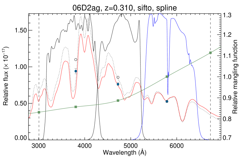
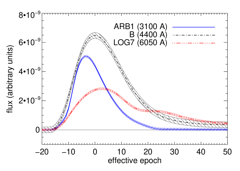
The method used to adjust the SED is similar to that described in H07: we multiply the SED by an interpolating cubic spline under tension (), with the spline knots placed at the effective wavelengths of the observed filters. In order to ensure that the SED remains positive, we work in log space. An example is shown in figure 1. We experimented with a variety of functional forms to smoothly scale the spectrum in place of splines, and found similar results using linear or higher-order polynomial interpolation.
3.1. The stretch model
In the SiFTO model, , the stretch in filter , is not necessarily the same as . Our model for this correction is , where and are the effective rest frame wavelengths of and the filter for our fiducial, SED at :
and similarly for , although for the latter the redshift of the SN needs to be taken into account. Given the stretch in the observed filter, we adjust the corresponding flux normalization by multiplying it by the ratio:
This gives observer-frame flux in each observed filter. There is still only one light-curve shape parameter, .
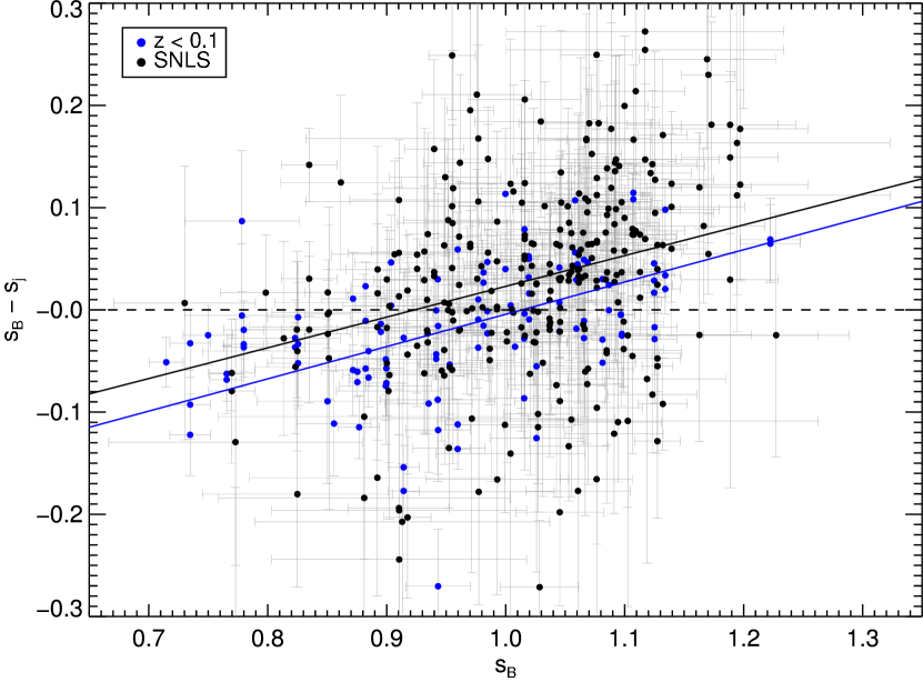
The stretch function is represented by a spline, and is derived from both external and SNLS SN Ia data as follows. We require that at least one of the filters lie within 250Å of rest frame in order to ensure that is well determined. However, in addition to fits to individual filters, we also consider nearest neighbor combinations of the SNLS filters (, , and ), and include the SN if the mean wavelength of these filters meets the above requirement. In these cases is well bracketed, so is also well constrained. The stretch and (mean) rest-frame effective wavelength is recorded for each fit. The results are shown in figure 2.
Alhough the relationship between and varies slightly with wavelength, a general trend is apparent: is typically smaller than for small and larger for large . It is also apparent that the low-z and SNLS samples probe different ranges in (with the low-z sample containing more low- SNe and the SNLS sample more high- SNe). This is not surprising given expected selection effects and the possibility of an evolving population (e.g., Howell et al., 2007).
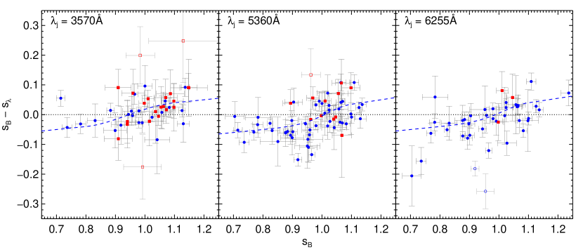
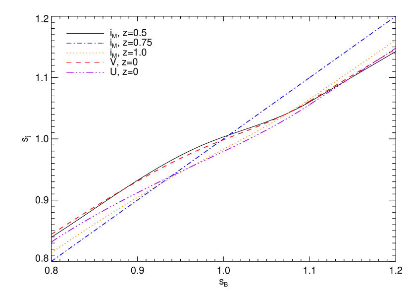
To model the trends, we fit the relation between and using least-squares in Å wide bins, using a cubic spline with three knot points in smoothly joined to a linear relation at low and high . Each wavelength bin contains 20–60 datapoints; three example bins corresponding to , and are shown in figure 3. The relationship between and at any intermediate can be found by linearly interpolating the fit coefficients in wavelength. We do not probe all areas of equally well, with clusters around the low-z filter mean-wavelengths; this is an area where larger samples of SNe Ia will be extremely beneficial. Examples of the derived function are shown in figure 4.
We can test the necessity of this more complex treatment of stretch by applying the SiFTO model to the photometry from A06 (see §7.3 for more details). For the model described above, we find a of 2890 for 2822 degrees of freedom. If we remove the wavelength dependence of the stretch model the climbs to 3037, and if we instead use a purely linear model in place of the splines, the is 2935. These correspond to a decrease in likelihood by a factor of 70 and 3, respectively. However, we note that the cosmological results and the scatter around the best fit are almost identical in all three cases ( mag difference in the RMS). The lack of improvement in the relative distances can be interpreted as an illustration of the difference between a light-curve fitter and a distance estimator.
3.2. Constructing the SED model
The starting point for our base SED model is an updated version of the time series of spectral templates of H07 which incorporates the additional low-z spectroscopy presented in Matheson et al. (2008). The procedures of H07 are designed so that the relative strengths of adjacent features are correct, but are not intended to adjust the broadband colors or their evolution with time, so some modification is necessary. We developed a set of light-curve templates that are used to address this issue. These templates are purely an intermediate step, and play no role in the fitting process once is determined.
There are many approaches one might use to build the templates. For SiFTO, we construct a set of synthetic filters and then use SN data to build light-curve templates in each of these filters. We then adjust to match these templates using interpolating splines as described earlier. This process requires -correcting the observed data points, which are at a variety of redshifts, to the nearest template filter. Since the -correction depends on the model SED, this procedure is carried out iteratively. We follow a fairly standard approach by parameterizing each light-curve template as a set of cubic splines with the knot points tuned by hand to best describe the data (e.g., Goldhaber et al. (2001)). The number of knots ranges from 3 (for poorly constrained filters) to 8 for the redder filters which have a more complex template. Since cubic splines are used, the templates are only smooth up to first order in the derivatives; applications which require higher degrees of smoothness should not use SiFTO. The splines are joined smoothly to a polynomial at early times, and an exponential decay function at late times. The location of the join can be set for each filter; generally the early time polynomial joins the splines around epoch , and the exponential tail around , although in some filters this is much lower due to the lack of good late-time data. The early-time polynomial is of the form , where is the date of zero flux (i.e., the date of explosion). Therefore, for our template, the colors of the SN at early times are not constant in all cases due to the cubic term. We require the polynomial coefficients to be positive to ensure that the early time light-curve increases monotonically at early times, which we expect on physical grounds. Linear and quartic terms were not found to improve the fits.
The choice of which filters to construct templates in is fairly arbitrary. If only low-z data is used for training, then a natural choice would be the Landolt filters, redshifted slightly to the mean redshift of the sample. Since we use both low-z and SNLS data, this is no longer optimal. We want to make use of information blue-ward of , and it is also useful to insert filters between the more widely spaced Landolt filters to make better use of our observations and improve the smoothness of the model.
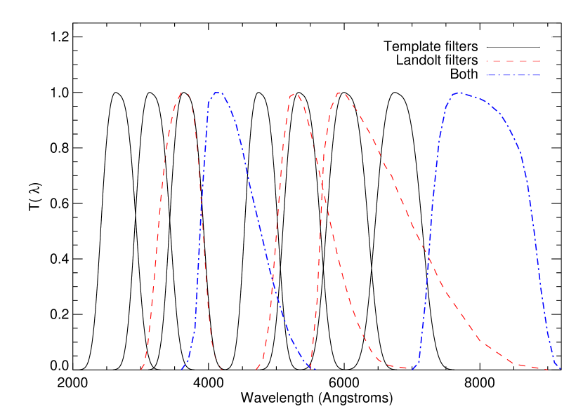
We use a set of synthetic logarithmically spaced filters between 4800 Å and 6800 Å, and also include and . In addition, we include three bluer filters which are blueshifted and widened versions of the first log filter. The filter is included to make it easier to compare the resulting template with previous work, and to ensure well-behaved boundary conditions while building . We do not use the part of the model redder than 7100 Å when applying SiFTO to observations because our stretch parameterization is not expected to work well. The synthetic log filters are denoted as LOG5 – LOG8, and the three bluer filters are ARB0 – ARB2. The light-curves in ARB0 and ARB1 are determined purely by SNLS data. Our filters are shown in relation to the Landolt filters in figure 5. ARB2 matches (but is slightly redder), LOG6 roughly matches , is split up into two narrower filters which are better matches to the SNLS observations (LOG7 and LOG8), and there is an additional filter between and (LOG5). The filters are summarized in table 1. The SiFTO model should only be used for observations from 2700 to 7100 Å (rest frame).
We use cubic terms in the early-time polynomials for the ARB0, ARB2, and LOG5 filters. For ARB0, including this term reduces the of the template fit to our training sample from 171 for 155 degrees of freedom to 167. For ARB2 the goes from 4613 to 4515 for 1605 degrees of freedom, and for LOG5 from 2280 for 1004 degrees of freedom to 2001. We caution that these values do not incorporate the template error snake as described in §3.3, and hence we do not expect the reduced to be close to unity. It is difficult to evaluate how significant the improvements in the are, since the process of building the error snake involves inflating the errors to take into account the residuals from the model. However, in the other filters the best fit value of the cubic coefficient is zero.
The procedure of building the templates in each filter is as follows: First, all of the data is fit using SiFTO with the current version of . The observed data is - and MW-extinction corrected to the best matching template filter, and the timescale is normalized using and the stretch in each filter . The data points from each SN in each filter are normalized to an arbitrary value in order to remove the colors of the individual SNe from the template. The templates are then fit to the datapoints in each filter, and is adjusted using the spline procedure to match the model. The procedure is then iterated until convergence, which typically requires iterations. We also adjust the template so that represents the peak flux in , and adjust so that the mean over our training sample is unity.
It is convenient for our template to have roughly the colors of a fiducial SN Ia. Given the asymmetry of the color distribution we use the median color to define these values. There is no single SN with exactly this color, and if there were it would not constrain all of our template filters. Therefore, we take the mean 10% of the SN closest to the median color to define each color, and use this in the normalization process above. Note that this process does not affect the resulting light-curve fits as long as sharp, unphysical gradients are avoided. Changing the colors individually by up to 0.3 mag has no effect on the resulting fits because our procedure adjusts the SED template to match the observed colors.
With the above ingredients, we can write as
| (5) |
where is the spline used to make the SED have the desired colors, and not that used to construct . is uniquely determined by the combination of the products, , and the observed filters. can then be used to evaluate the flux in any desired filter, and not just those actually observed.
| Filter | aaThe effective wavelength for this filter when observing a fiducial SN Ia at . | FWHM | bbThe epoch of the join between the splines and the polynomial early form, relative to the epoch of maximum. | ccThe number of internal knots in the spline between and | ddThe epoch of the join between the splines and the exponential late form, relative to the epoch of maximum. | |
|---|---|---|---|---|---|---|
| ARB0 | 2689 | 2798 | 529 | 3 | 12 | |
| ARB1 | 3187 | 3206 | 530 | 4 | 25 | |
| ARB2 | 3685 | 3704 | 510 | 5 | 30 | |
| B | 4413 | 4330 | 893 | 6 | 50 | |
| LOG5 | 4784 | 4755 | 497 | 5 | 41 | |
| LOG6 | 5382 | 5363 | 559 | 6 | 48 | |
| LOG7 | 6055 | 6030 | 628 | 6 | 50 | |
| LOG8 | 6812 | 6854 | 707 | 7 | 47 | |
| I | 8060 | 8008 | 1526 | 7 | 47 |
Note. — Information about the template filters and the functional form used to fit each filter when deriving . Except for and , these filters are synthetic. These values are essentially hand-tuned.
3.3. The template error snake
SiFTO incorporates an estimate of the uncertainty in . This represents both the uncertainty in our modeling process, and, much more importantly, some measure of the intrinsic variability of SNe Ia. SALT2 and MLCS2k2 also incorporate an error snake, but some older fitters do not. The uncertainty in the template is very important when fitting low-z data, where the photometric uncertainties can often be quite small. It also plays a critical role when evaluating and observations of high-z SN, where the model is more poorly constrained. We tabulate the template error at the wavelengths of each of the template filters in one day bins and then linearly interpolate between these errors in wavelength space to get the error in the SED, which gives us the term in equation 4.
There are several methods used to derive the error snake, which give similar results. The most direct approach is to fit all of the SNe using SiFTO, and then determine the additional error that would make the of the data relative to the model be 1 per degree of freedom. The difficulty with this approach is that at some epochs the measurement errors of individual observations dominate the scatter. The SNLS error bars are roughly constant with epoch in flux space because it is a rolling search, but a 10% variation in the template flux at any given epoch is much larger in absolute flux at peak than at late or early times. Therefore, measuring the same relative variation at late times is more difficult, requiring an accurate cancellation of two numbers subtracted in quadrature. Compensating for this fact is the tendency of the template error to be larger in relative terms at late times which partially arises from the fact that we have renormalized the fits to each SN at peak. In order to improve our sensitivity at late and early epochs, we adopt a slightly modified procedure. In the core of the light curve ( to days) we use the method directly, but at late and early times we substitute a measure based on the RMS, but multiplied by the ratio between the result and the RMS as measured in the core. The results of this procedure are generally quite similar to that of the raw method (within about ).
The other method we consider is to use bootstrap-with-replacement to estimate the template errors. This gives similar results, but the + RMS approach is more robust and slightly more conservative in that it gives larger errors (by on average), so we use this for our final model. The error snake is used iteratively using the template construction process. Some examples are shown in figure 6.
Since we usually have a large number of observations in each epoch bin for each filter, the formal statistical error in how well we can measure the mean template is much smaller ( times) than the template error we quote. Some of this is probably due to failures in the photometry, uncertainties in the -corrections, and inconsistencies between different samples. However, looking at any of these in detail (for example, by considering only data from a single source such as SNLS, or looking at SN in a narrow redshift range where -correction uncertainties are less important in a relative sense), none of these effects is the right order of magnitude to explain the observed scatter. We conclude that SN variability is the dominant factor in the template error, except in our bluest artificial filter where the sample is small.
Like SALT2, our error snake does not incorporate off diagonal terms – i.e., the residual from the model at a given epoch is assumed to be uncorrelated with nearby epochs. Given the complexity of our model space, the current data set does not provide robust constraints on these terms. MLCS2k2, which has a simpler model and does not work with a SED, includes off-diagonal terms with simplifying assumptions.
3.4. Modeling systematics using SiFTO
Modeling of systematic errors is becoming increasingly important for SN cosmology. One issue which has been neglected is that because our SN model is empirically derived from SN data, the effects of the systematics on the model must also be considered in the error budget. This is important even if no high-z data is used in the training. An advantage that SiFTO has over most other light-curve fitters is that the effects of epoch-independent systematics can be studied simply by re-deriving the color relation, rather than having to fully retrain all aspects of the model. For example, a change in the SNLS zeropoint data does not affect the SED model because during the training process the data from each SN is normalized to an arbitrary level. It will, however, affect the relation between the measured colors of the SN population. Approaches which fold the modeling of SN colors into the model derivation more directly (SALT/SALT2, MLCS2k2) do not have this luxury.
This does not apply to any effect which can change the shape of the light curve, such as uncertainties in the filter responses. However, in most cases these are second order effects compared with the changes in the derived color relation. This makes systematic analysis with SiFTO comparatively easy.
4. DATA
Our training sample consists of photometry for nearby SNe Ia from the literature as well as high-redshift SNLS observations. The low-z data generally has higher signal-to-noise ratios, but are also much more heterogeneous. More importantly, the SNLS data offers considerably better wavelength coverage than the low-z sample, both in the near-UV and between the standard Landolt filters. Furthermore, the rest-frame band data from SNLS is better calibrated and more reliable than that from the low-z data.
The photometric references of the 72 low-z SNe used in this paper are given in table 2. We have not included sub-luminous (SN 1991bg-like) SNe Ia in our sample because they are not well represented by our base SED, and have excluded extremely peculiar SNe such as SN 2002cx (Li et al., 2003). Furthermore, we have not included all of the available photometry for every SN. In cases where photometry is available from multiple sources, we compare the light-curves from multiple bands and, if they are not consistent, choose some subset of the sources. We try to choose the photometry that has the best coverage, or that from the data source with the most other SNe (i.e., we prefer observations from a large sample like Jha et al. (2006)). We also exclude individual bands on a SN by SN basis where the photometry seems to be internally inconsistent or has additional problems (e.g., the band data for SN 1999ee).
In addition we use 98 high-redshift SNLS SNe from the first three years of the survey. Our training process requires that the peak of each observed filter be fairly well constrained so that we can re-normalize the light-curves accurately, a necessity since we do not impose a color relation during the training process or fits. Therefore, to use an individual bandpass for a SN, we require that it have at least one datapoint within 5 rest-frame days of maximum. This requirement is far more stringent than is necessary to carry out a cosmological analysis, so less than half of our high-z data are used in the training process. We use only SNe with firm spectroscopic identification. The H07 template makes use of SNLS spectra, which are particularly critical when constraining the near-UV SED. As was the case for the low-z sample, we exclude SNe which are known to be unusual, such as the super-Chandrasekhar mass 03D3bb (Howell et al., 2006).
For SNLS, we adopt the radially-dependent SAGEM filter scans for the MegaCam filters, corrected for the f/4 converging beam and incorporating the Mauna Kea extinction curve at the mean survey airmass of 1.2. A06 used radially averaged versions of these scans. For the low-z data we adopt the Bessell (1990) realization of the Landolt filter functions. Ideally we would have natural system magnitudes and bandpasses for all of the low-z photometry, but this information is generally not available. Hopefully this will not be the case for future low-z data sets. Currently we do not implement any airmass dependence in our assumed filter functions, since tests show that this is negligible in comparison with the other bandpass uncertainties.
| Name | Filters | Source aa Photometry References: H91 Hamuy et al. (1991), P87: Phillips et al. (1987), W94: Wells et al. (1994), H96: Hamuy et al. (1996a), L98: Lira et al. (1998), J99: Jha et al. (1999), R99: Riess et al. (1999), S99: Suntzeff et al. (1999), K00: Krisciunas et al. (2000), K01: Krisciunas et al. (2001), S01: Salvo et al. (2001), S02a: Strolger et al. (2002), S02b: Stritzinger et al. (2002), K03: Krisciunas et al. (2003), V03: Vinkó et al. (2003), A04: Altavilla et al. (2004), K04: Krisciunas et al. (2004), P04: Pignata et al. (2004), L05: Leonard et al. (2005), R05: Riess et al. (2005), ER06: Elias-Rosa et al. (2006), K06: Krisciunas et al. (2006), J06: Jha et al. (2006), L06a: Lair et al. (2006), L06b: Li et al. (2006), T06: Tsvetkov (2006), K07: Krisciunas et al. (2007), P07a: Pastorello et al. (2007a), P07b: Pastorello et al. (2007b) |
|---|---|---|
| 1981D | H91 | |
| 1986G | P87 | |
| 1989B | W94 | |
| 1990N | L98 | |
| 1990O | H96 | |
| 1990af | H96 | |
| 1992ae | H96 | |
| 1992al | H96 | |
| 1992bc | H96 | |
| 1992bg | H96 | |
| 1992bh | H96 | |
| 1992bl | H96 | |
| 1992bo | H96 | |
| 1992bp | H96 | |
| 1992br | H96 | |
| 1992bs | H96 | |
| 1993B | H96 | |
| 1993H | H96, A04 | |
| 1993O | H96 | |
| 1993ag | H96 | |
| 1994M | R99, A04 | |
| 1994S | R99 | |
| 1994ae | R05, A04 | |
| 1995D | R99 | |
| 1995E | R99 | |
| 1995ac | R99 | |
| 1995al | R99 | |
| 1995bd | R99, A04 | |
| 1996C | R99 | |
| 1996X | R99, S01 | |
| 1996ab | R99 | |
| 1996bl | R99 | |
| 1996bo | R99 | |
| 1997E | J06 | |
| 1997bp | J06 | |
| 1997dg | J06 | |
| 1997do | J06 | |
| 1998V | J06 | |
| 1998aq | R05 | |
| 1998bu | J99, S99 | |
| 1998dx | J06 | |
| 1998es | J06 | |
| 1999aa | J06, A04, K00 | |
| 1999ac | J06 | |
| 1999aw | S02a | |
| 1999cc | J06, K06 | |
| 1999cl | J06, K06 | |
| 1999dk | K01, A04 | |
| 1999dq | J06 | |
| 1999ee | S02b | |
| 1999ek | J06, K04 | |
| 1999gd | J06 | |
| 1999gp | J06, K01 | |
| 2000ca | K04 | |
| 2000cn | J06 | |
| 2000dk | J06 | |
| 2000fa | J06 | |
| 2001V | V03, L06a | |
| 2001ba | K04 | |
| 2001bt | K04 | |
| 2001cn | K04 | |
| 2001cz | K04 | |
| 2001el | K03 | |
| 2002bf | L05 | |
| 2002bo | K04 | |
| 2002er | P04 | |
| 2003cg | ER06 | |
| 2004S | K07 | |
| 2004eo | P07b | |
| 2004fu | T06 | |
| 2005am | L06a | |
| 2005cf | P07a |
5. RESULTS OF THE TRAINING
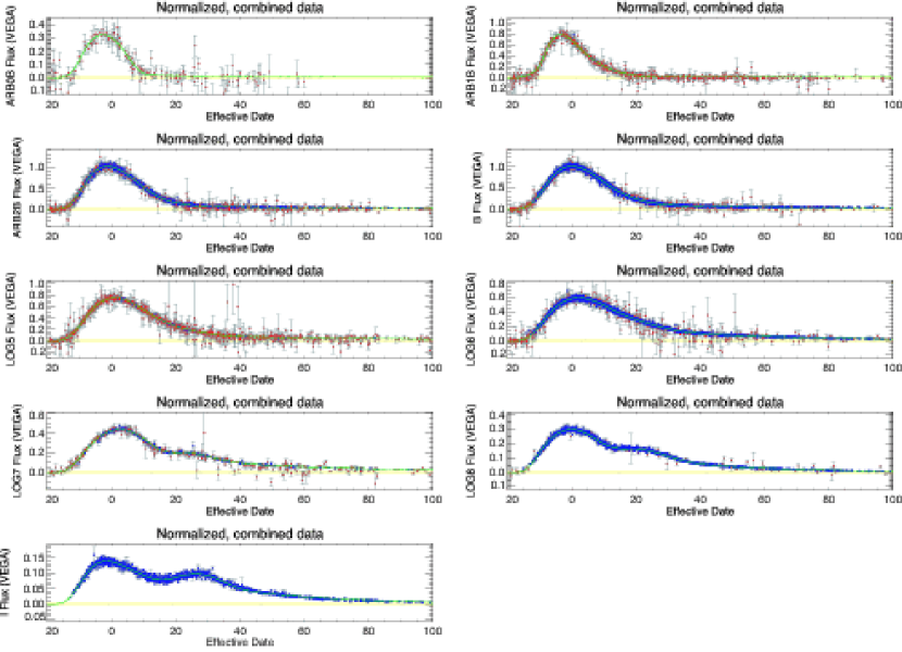
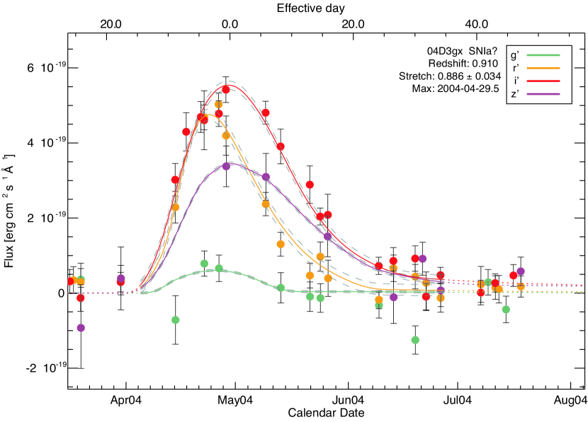
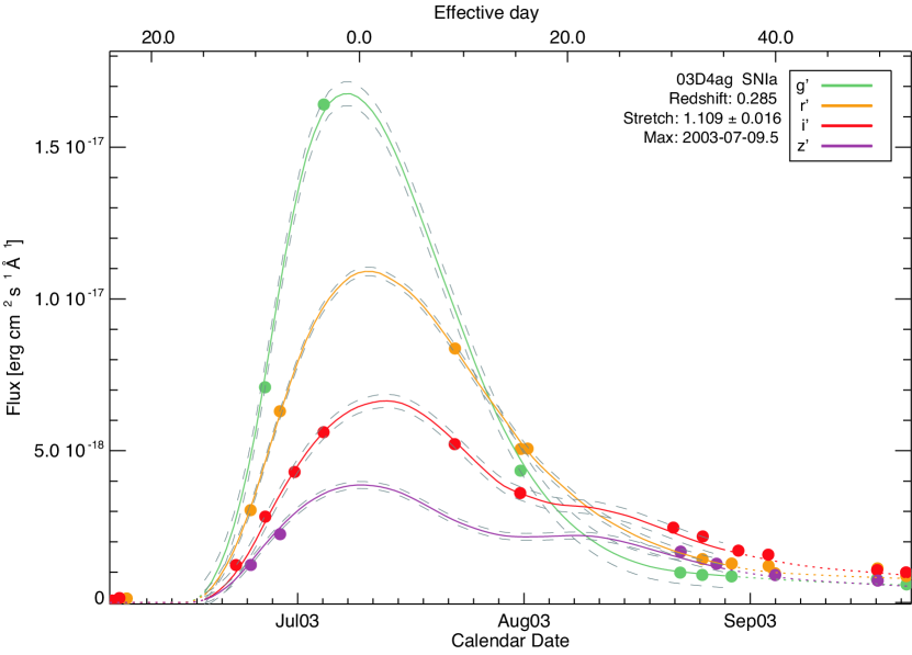
The light-curve templates can be seen in figure 7. The different manner in which the SNLS and low-z data sets sample wavelength space is clear – only the SNLS data offer any constraints blue-ward of (ARB0 and ARB1), and the wavelength region between and (LOG5) and and (LOG7), while the nearby data provide most of the constraints in . However, in the filters where substantial coverage is provided by both sets (LOG3, , LOG6), the agreement is impressive. In addition, the homogeneity of SNe Ia light curves is also apparent. Note that in the band extensive culling has been performed because many SN do not match the template. This is acceptable because we are only including to ensure well behaved boundary conditions, and do not use this part of the model directly when applying the model to SN observations. Example fits to high and low redshift SNLS SNe are shown in figures 8 and 9 (the same SN were used as examples in G07).
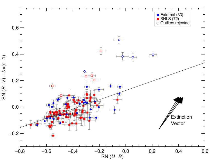
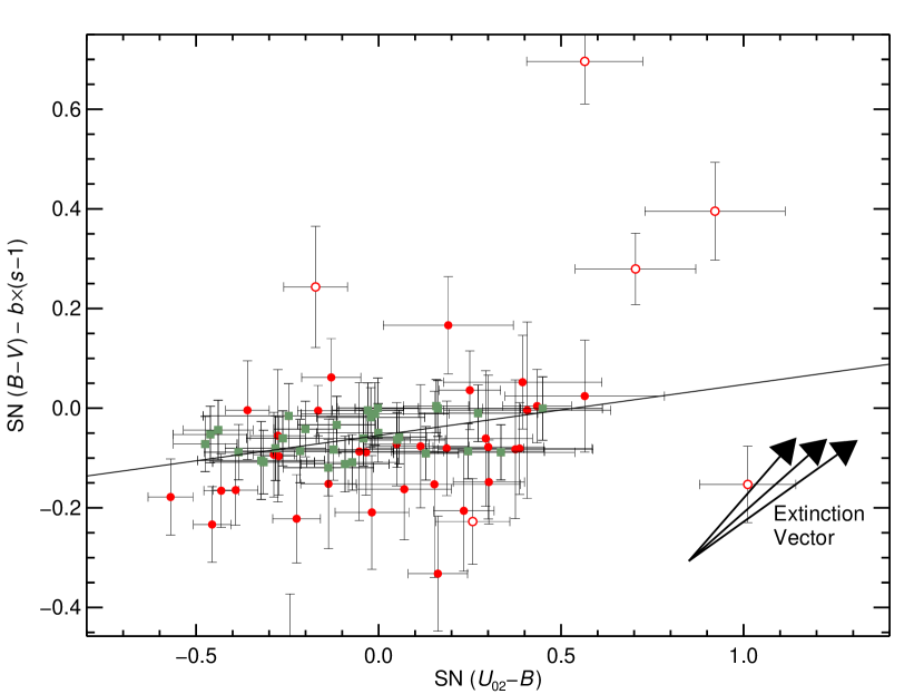
The parameters of the color relations used to determine parameter (equation 2) are given in tables 3 and 4, and the and relations shown in figures 10 and 11. The relation is derived from 72 SNLS and 33 low-z SNe, and the relation from 63 SNLS SNe. Here, because there are few SNe with both and measurements, we include data with no rest-frame observations by using their colors to predict , incorporating the additional uncertainty due to and the appropriate covariances. The requirements to be included in the color relation fit are less stringent than those required to be used when measuring since we do not require that the fits to each filter be strongly constrained in isolation. The primary limitation is instead that most SNe do not have simultaneous measurements of and . Carrying out this test with SALT2 gives similar values for the parameters. It is interesting to consider the residuals from the versus relation. The slope of the dominant relation is clearly inconsistent with that expected from extinction. However, there are a number of outliers that are displaced in a direction that could be explained by extinction. This leads us to hypothesize that the color relations for the majority of SNe in our sample are dominated by intrinsic effects, with a minority instead dominated by dust.
Following G07, we can get some feel for how useful extending the model blue-ward of is be comparing measurements of if the model is cut at different wavelengths. This is shown in table 5 for 04D3cy () and 04D3gx (). The errors include statistical uncertainties, template errors, and -correction errors as described in H07. The benefits for the higher redshift SN are clear.
| Parameter | Value | Error |
|---|---|---|
| SNLS + low-z | ||
| 0.352 | 0.049 | |
| 0.218 | 0.064 | |
| 0.051 | 0.007 | |
| 0.055 | 0.005 | |
| SNLS only | ||
| 0.435 | 0.067 | |
| 0.302 | 0.076 | |
| 0.067 | 0.008 | |
| 0.044 | 0.006 | |
| low-z only | ||
| 0.259 | 0.090 | |
| 0.145 | 0.132 | |
| 0.037 | 0.016 | |
| 0.071 | 0.011 | |
| Parameter | Value | Error |
|---|---|---|
| 0.121 | 0.050 | |
| 0.172 | 0.138 | |
| 0.110 | 0.027 | |
| 0.050 | 0.008 |
Note. — The coefficients for the vs. color relation.
| bands | aaThe weight given to when forming . | bbThe weight given to when forming . | ccThe weight given to when forming . | ||
|---|---|---|---|---|---|
| SNLS-05D3lb | |||||
| 3980 Å | 0 | 0 | 1 | ||
| 3250 Å | 0 | 0.69 | 0.31 | ||
| 2700 Å | 0.43 | 0.40 | 0.18 | ||
| SNLS-04D3gx | |||||
| 3980 Å | 0 | 1 | 0 | ||
| 3250 Å | 0 | 1 | 0 | ||
| 2700 Å | 0.60 | 0.40 | 0.00 | ||
Note. — The errors in for two SNLS SNe when the model is cut at different wavelengths. The cuts correspond to including all of , removing , and removing . Note that the rest-frame is not measured for SNLS-04D3gx. The improvement in the measured color for 04D3gx when is added is due to the improved constraints on the other light-curve parameters such as the date of maximum, even though it is not formally used in the color.
The stretch is only defined relative to some fiducial template, and does not have any independent meaning when comparing different fitters, or even different versions of the same fitter. Instead, a variable like can be used which has a more physical definition.111The quantity is the amount in magnitudes which the band light curve has dimmed 15 rest frame days after peak. However, in practice, because light-curve fits are relatively insensitive to the exact shape of the light-curve template near peak, even is somewhat ambiguous, and will change when the light-curve model is updated. Therefore, we simply provide the relation between and for our template:
This relation should not be used for precision work, such as attempting to combine data fit with different packages.
5.1. Comparing the color parameters from SNLS and low-z data
For the color relation, we can split the sample into low-z and SNLS data as a test of SN evolution. This results in the values given in table 3. There is some tension between the values. However, this only includes statistical errors, and systematics are expected to be of similar importance. The details of our systematics analysis will be presented with our cosmological results elsewhere, but it is useful to summarize some of the more important contributions. The most important uncertainties arise from the uncertainty in the magnitudes of our flux standard (Vega) on the Landolt system (which affect our -corrections) and the uncertainty in the calibration of the low-z data. The former are dominated by the raw observational uncertainties of Vega from Johnson & Morgan (1953). To determine how well calibrated the low-z data is to the Landolt system, we compare photometry of the same SNe obtained by different observers (e.g., Riess et al., 1999; Jha et al., 2006), and conclude that there is a global zeropoint uncertainty of about 0.015 mag in for each survey. For the situation is more complicated. As noted previously, observer frame data is more difficult to calibrate than , so we double this value to 0.03 mag in this filter. However, as it turns out the zeropoint uncertainty dominates over , at least partially because it affects both and .
In order to test the effects of these systematics, we adjust the relevant parameter (e.g. the zeropoint), then re-derive the SiFTO model and color relations. We then consider the change in to be the resulting systematic in , etc. For the uncertainties in the magnitude of Vega, we find and . We do not include because its value is likely to simply test the homogeneity of the data sample rather than be a good test for evolutionary effects. For the zeropoints of the low-z data, we find and . Other, smaller, contributions include the uncertainty in the MegaCam and Landolt bandpasses and the MegaCam zeropoints. The latter is particularly important for , giving for sub-1% zeropoint uncertainties.
Putting this information together, we conclude that , , and . The resulting is 4.57 for 3 degrees of freedom, which is expected to occur by random chance in the case of no evolution 21% of the time.
6. HOW CLOSE TO PEAK DO WE NEED DATA?
One question we can ask of our model is whether or not it can predict the peak luminosity of the SN when we have no observations at that epoch. That is, how well can our model extrapolate from late time observations to the peak? In principle, the template error snake should allow us to handle situations where there is little or no data near peak, since the result will simply be a measurement with very large errors. However, the error snake is not known perfectly, so we would like to test this statement. Most SN cosmology analyses have required that SNe have data near peak, but the exact value used for this cut varies from paper to paper and is usually not explained. The previous generation of SN fitting packages, which often did not incorporate template errors, frequently produce implausibly precise results when used in this situation.
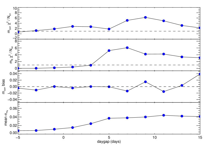
Our test is based on real observations; a test on simulated data is currently likely only to be useful as an internal consistency check. We collect a sample of very well sampled, high-S/N light-curves with data well before peak, and then, for each SN, compare the results of the fits to all of the available data to those where we steadily remove more and more photometry from around the peak. We parameterize this by the daygap, defined as the epoch of the first included point relative to the date of maximum, and explore the range from 5 to +15 days. Our sample consists of the 11 low-z SNe: 1992A, 1995D, 1999aa, 1999dq, 1999ee, 2000E, 2002bo, 2002er, 2003du, 2004eo, and 2005cf. Even these SNe generally do not have data before day 10, which is why we have not tried to answer the complementary question of how well our model can predict the peak magnitudes of SNe Ia if we only have pre-maximum observations.
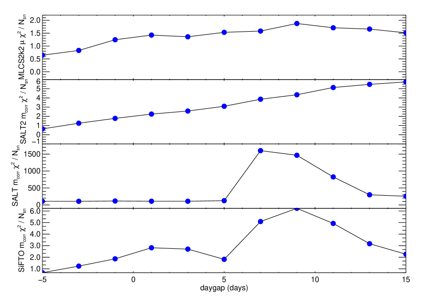
There are two things we want to test: that the results are unbiased, and that the errors reflect the missing data appropriately. For the latter, we compare the of the difference between the light-curve parameters for the full light-curve, and for those at various values of the daygap. Since the different fits to the same SN should be positively correlated, we will probably slightly over-estimate our errors. This test is sensitive to small calibration difficulties that arise when different telescope/detector systems observe different parts of the light-curve, which is frequently the case with low-z data. This will artificially inflate the differences. Therefore, the precise value should not be taken too seriously; what we are looking for are sharp changes in the .
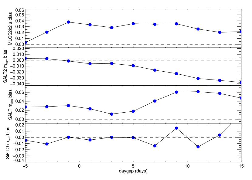
The most important parameter to test is as defined in equation 1, which is used to construct the Hubble diagram. Rough numerical simulation suggests that bias values larger than about 0.02 are significant. Most of the variables show relatively little structure in their , so we only present the two given in figure 12. First, the of the peak magnitude in rises sharply around day 5–10 after peak. Second, while this effect is also visible for , the effects are slightly muted. Our tests show little evidence for bias in the corrected peak magnitude. Based on the -like test, a good policy is to require data within days of peak when using SiFTO.
Note that the accuracy of the derived parameters does degrade considerably as the daygap is increased in all parameters (see the bottom of figure 12), so SNe with no data near peak will contribute relatively little information to the Hubble diagram. We carry out the same test with other fitters in §7.2, and find generally similar results.
7. COMPARISONS WITH OTHER FITTERS
In this section, we compare the results of SiFTO with those of other fitters, particularly the published versions of SALT and SALT2. Our main focus will be on comparisons of SiFTO, SALT2, etc. when they are used as distance estimators rather than as light-curve fitters. There are a number of non-SN related settings that affect this comparison (i.e., the assumed filter response of the Landolt filters222SALT and SALT2 follow A06 in using blue-shifted versions of the Bessell (1990) responses, while SiFTO does not., etc.), so this comparison is not entirely fair. In § 8 we present the results when these differences are removed which provides a much more accurate test of how different the results of the fitters really are.
We discuss MLCS2k2 in a more limited fashion in this section, keeping in mind the following limitations: First, MLCS2k2 makes use of a number of priors which should be accounted for in any detailed comparison, and which in principle should be modified for the particular data set under consideration. Second, it fits in magnitude space, which will introduce a bias when comparing low signal-to-noise data333Subsequent to this writing, a version of MLCS2k2 which works in flux space was kindly provided by G. Narayan (2007, private communication). However, it does not address the other issues.. Finally, the current version of MLCS2k2 does not properly handle the case where more than one observed filter maps to the same rest frame Landolt filter. This limits the sample size that can be compared using SNLS data.
We also consider comparisons of the Hubble diagram. All of the fitters require that some additional uncertainty be added to the luminosity distances when computing the best-fit cosmology. This is often referred to as “intrinsic scatter” or “intrinsic dispersion,” and presumably reflects our imperfect understanding of SN Ia. We denote this quantity by , and find mag for SiFTO. Comparing the values of for the different fitters is not currently a useful mechanism for comparison. The issue lies with the limitations of the template error snakes, which are difficult to determine and are very sensitive to how accurate the input flux errors are measured. In addition, currently both SiFTO and SALT2 do not include off-diagonal terms in the error snake (i.e., different epochs are considered uncorrelated), an assumption which is clearly not true. This is particularly an issue for SALT2, which imposes the color relation during the fits. Both effectively absorb this unknown into , and there is no reason to expect this to affect both equally. Therefore we limit ourselves to the more robust comparison of the RMS of the resulting Hubble diagram. However, the RMS also includes the effect of measurement errors, so is only useful as a comparison statistic if precisely the same set of input data are used for all fitters. A complication is that there is considerable overlap between the data used to measure the RMS and that used to derive the SiFTO model; the same issue applies to SALT2, MLCS2k2, and (to a lesser extent) SALT. However, we note that SiFTO/SALT/SALT2 make absolutely no use of relative distance information as part of the training process.
7.1. Comparison of SiFTO and SALT2 light-curve fits
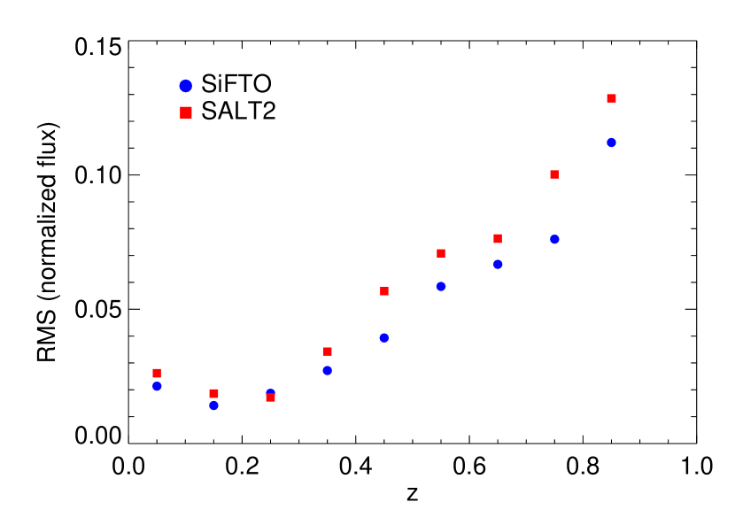
We begin by comparing SALT2 and SiFTO as light-curve fitters – that is, in terms of how well they fit the available photometry rather than in terms of the precision of their relative distances. Here we do have the problem that the training process is specifically designed to reduce the scatter of the input photometry with respect to the model, so it is beneficial to train and test the models with disjoint data sets. We have carried this process out for SiFTO by randomly splitting the training sample in half (giving about 90 SNe for both testing and training), training a set of templates on the first half, and then applying that model to the second half. We then look at the residual between the model and input flux normalized so that the predicted peak flux in each filter is unity. Because this includes observational errors, we split this up into redshift bins (). In order to mitigate photometry failures, we sigma-clip the residuals at for both fitters. The results are shown for SALT2 and SiFTO in figure 13 using the same photometry. This comparison is unfair in two ways: first, the splitting into disjoint training and testing samples has not been carried out for SALT2. Second, the SiFTO model has more free parameters since a color relation is not imposed during the fitting process. Nonetheless, the two fitters give comparable results.
7.2. Comparisons using low-z data
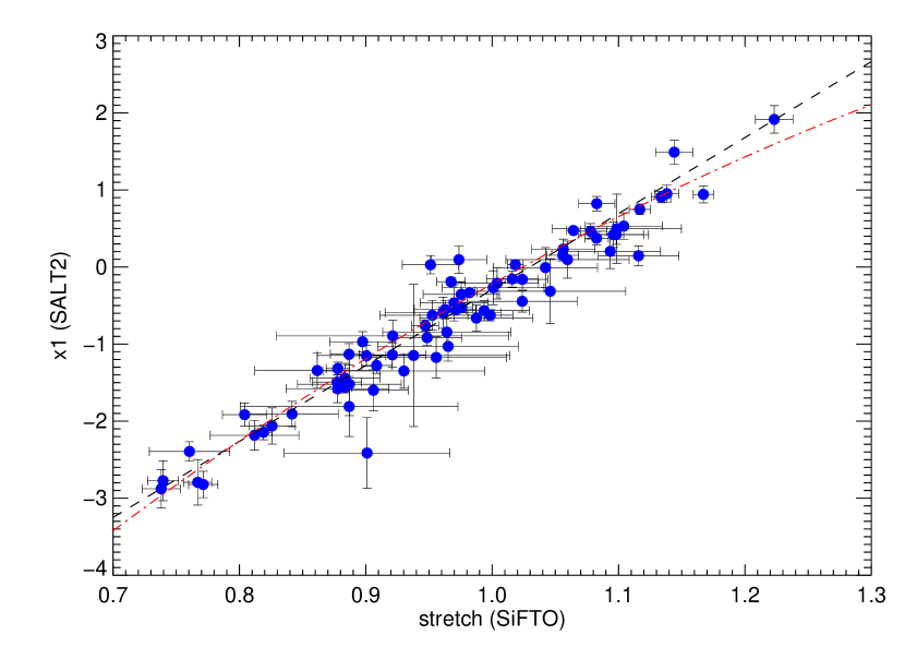
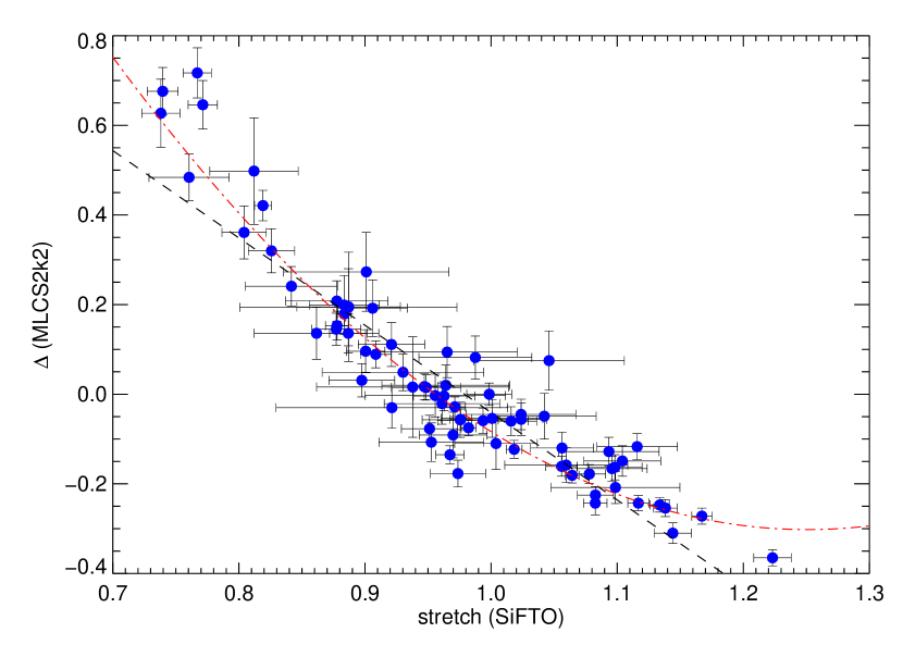
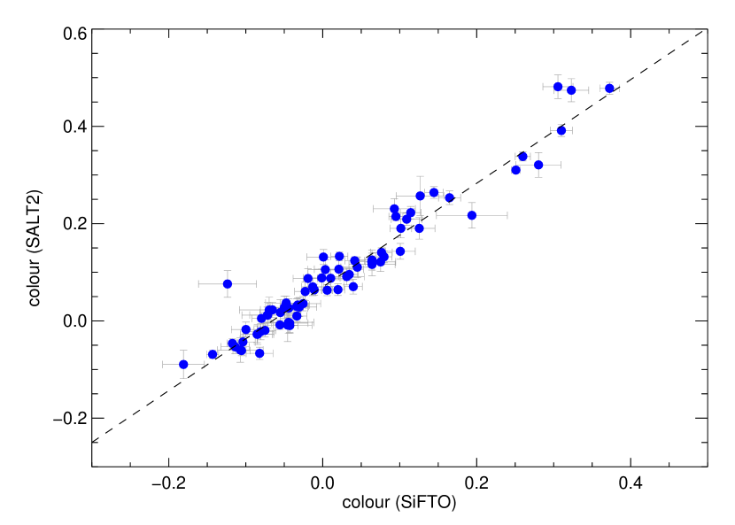
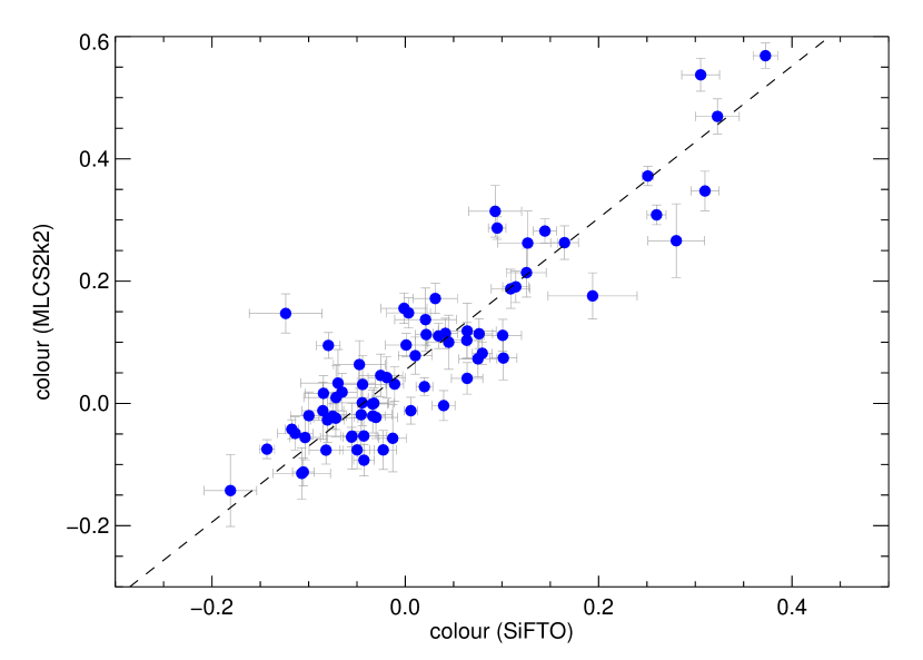
The different light-curve fitters generally agree quite well on the derived light-curve parameters, particularly when the MCLS2k2 priors are removed. Examples are shown in figures 14 and 15. We generally do not expect perfect agreement between the different light-curve parameters, but only that there be a clear relation between the values. This is particularly true when discussing measures of the light-curve shape, which are defined very differently, and SN color, which can have an arbitrary offset related to the intrinsic color of the fiducial SN Ia. The data set for this comparison is 78 low-z SNe from the literature, using the same general requirements as were used in Conley et al. (2007), although the sample here is larger because we can include SNe which are not in the smooth Hubble flow.
The derived parameters are clearly quite correlated between the different fitters, although there are a number of outliers in each relation. The comparison is consistent at about the 1% level globally, and since for most purposes only the relative distances matter, this is encouraging.
Next we turn to the RMS around the low-redshift Hubble diagram. We take the above sample, remove all SNe with , and then fit the Hubble diagram assuming and – the exact values are unimportant because of the limited redshift range of our test sample. The RMS values and are given in table 6. MLCS2k2 is not included in this test because of complications related to the interpretation of SN colors, which in turn is related to the question of whether or not the low-z Hubble flow is really smooth or has a Hubble bubble, something that MLCS2k2 favors and the other fitters do not (Conley et al., 2007) . Since we do not include a bubble in our test, this will tend to artificially inflate the RMS for MCLS2k2. However, we do perform the test using a larger data set below, where this issue is mitigated by a larger, higher-redshift sample.
| Method | RMS (mag) | (mag) |
|---|---|---|
| SALT | 0.156 | 0.134 |
| SALT2 | 0.158 | 0.129 |
| SiFTO | 0.155 | 0.119 |
Note. — The RMS and values for fits to the same low-z data, and assuming , . is not useful for evaluating the different fitters.
We find that the three fitters perform equally well on this data set. This is simultaneously encouraging and discouraging; it gives us confidence in the different fitters, but at the same time suggests that it is not easy to significantly improve the quality of the distance estimates for SN Ia beyond the level without some improvement in the training data set. Interestingly, when we perform the same comparison with high-z SNe, SALT2 and SiFTO do considerably better than SALT.
Finally, we can test the other fitters to see how well they fare if there are no data near peak, using the same method and set of 11 SNe as in § 6. It is particularly interesting to consider SALT, which alone among those discussed here does not have a template error snake. The bias values are shown in figure 16 and the -like test results in figure 17. MLCS2k2 performs the best in the -like test, which is also true for the individual fit quantities. MLCS2k2 and SALT display some bias even for low values of the daygap. One possible explanation is that both fitters would benefit from some improvement in their pre-maximum light-curve model.
We note that SALT does quite poorly in the -like test, as expected. Furthermore, we obtain similar results when we do not use the template error snake in SiFTO. The real lesson is then that including template errors plays a critical role in obtaining reliable fits when there are no data near peak.
7.3. Comparisons using high-z data
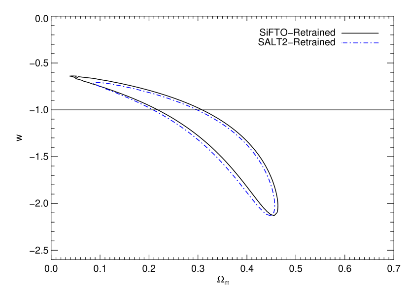
It is also interesting to compare the results of fits to high-redshift SNLS data. We first compare SiFTO to the published versions of SALT and SALT2. Because we can apply each fitter to the same photometry, again the best comparison statistic is the RMS of the resulting Hubble diagram around the best fit. The alternatives all have problems. In particular, comparing the resulting errors on the cosmological parameters is a badly flawed metric unless the fits are virtually identical, given the non-linearity of the parameter space. An additional complication occurs if the constraint contours impinge on a physically prohibited region, such as . Tests with synthetic data sets are perhaps useful as an internal consistency check, but we do not currently understand SNe Ia well enough for them to have any absolute meaning.
For this set we start with the set used in A06 and modify it slightly. We removed two SNe without solid spectroscopic type identification (04D2iu and 04D3is), one with photometry problems (03D4cn), and one which is probably SN 1991bg-like, and hence not well represented by any of the models (SN 1992bf). We also removed a number of SNe whose light-curves are poorly sampled (SNe 1997Y, 1998eg, 03D3bh, 03D4gl, 04D1ag). Finally, we added two low-z objects, SNe 2001V and 2002bf. This leaves us with a sample of 43 nearby SNe and 65 high-redshift ones.
We carry out three cosmological fits for each: a flat-Universe fit, a + fit, and a flat-Universe + fit. For the latter, we incorporate the SDSS baryon acoustic oscillations (BAO) measurements of Eisenstein et al. (2005), since these are marvelously orthogonal to the SN constraints. The results are given in table 7. A bootstrap analysis indicates that the error in the RMS for this sample is mag. From the perspective of the RMS test, SiFTO and SALT2 are indistinguishable, and both considerably outperform SALT. We also demonstrate the effects of not incorporating the filter in SiFTO, which worsens the RMS values at approximately the level. We note that the benefits of extending the model bluer than are greater for the third year SNLS sample than are shown here. This is probably a result of the fact that the exposure times have been increased, so our SNe now have better measurements of and hence have increased weight in our fits. The RMS including high-z data is slightly worse than if only low-z SNe are used, which simply reflects the larger observational errors of the distant sample.
| Fit type | RMS | Parameters |
|---|---|---|
| SiFTO | ||
| Flat | 0.161 | |
| + | 0.160 | |
| Flat + | 0.161 | |
| SiFTO w/out | ||
| Flat | 0.171 | |
| + | 0.170 | |
| Flat + | 0.172 | |
| SALT | ||
| Flat | 0.187 | |
| + | 0.187 | |
| Flat + | 0.188 | |
| SALT2 | ||
| Flat | 0.160 | |
| + | 0.160 | |
| Flat + | 0.160 | |
Note. — RMS values (in magnitudes) and resulting cosmological parameters for fits to the A06 photometry using SiFTO, SALT, and SALT2. Only statistical errors are included. The results of applying the SiFTO model limited to (excluding ) are also shown. As explained in the text, only the RMS should be used as a performance comparison statistic. The RMS has an uncertainty of mag.
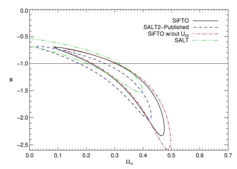
Some of the resulting constraints are shown in figure 18. We see that some differences remain between the fitters. We shall turn to the question of whether this reflects significant differences between the models in §8. A weakness of the RMS as a test statistic is that it is sensitive to outliers. Including iterative outlier rejection does not appreciably change the results.
We can perform a more limited version of this test including MLCS2k2, although given the caveats given earlier this is somewhat less certain and has a smaller sample size. We obtain the results of MLCS2k2 fits to the A06 photometry from Wood-Vasey et al. (2007). This is a subset of the full data set, with about 93 SNe in total. We therefore limit the SALT, SALT2, and SiFTO fits to the same sample. We do not include the ESSENCE SNe in this test. Carrying out a similar analysis as the above, the RMS for SALT is 0.179 mag, for SALT2 0.159 mag, for SiFTO 0.160 mag, and for MLCS2k2 0.205 mag. As noted for the low-z comparison, the MLCS2k2 value is somewhat inflated by the issue of the Hubble bubble. If we approximately remove this effect by hand, the RMS for MLCS2k2 is about 0.19 mag, so we conclude that its RMS is similar to SALT. Adjusting the priors to better match the survey properties of SNLS might improve the performance of MLCS2k2. It will be interesting to perform this comparison again once the issues surrounding SN colors have been resolved.
8. A BETTER COMPARISON BETWEEN SiFTO and SALT2
The differences between the SALT2 and SiFTO results on the A06 photometry reflect not only differences in the underlying model but also a variety of incidental settings, many of which are not related to SNe at all. While these differences are interesting, and play a role in the systematics error budget of our final result, here they simply obscure what we really want to know: what effect do the differences in approach have on the cosmological parameters?
We can try to answer this question better by using the same non-SN related settings for both fitters (filter functions, the magnitudes of Vega on the Landolt system, etc.). The published version of SALT2 was trained on the set of SNLS photometry available at the time using the MegaCam calibration of A06. There are now more SNLS SNe available, and the calibration has been improved. We can further enhance the comparison by training both fitters on exactly the same low-z and SNLS photometry, using the same filter functions assumed by SALT2 in SiFTO, and adding the additional low-z SNe provided by T. Matheson to SALT2.
Carrying out this prescription, we obtain the results in table 8 and figure 19. The results substantially closer to each other. This is very encouraging, and suggests that in terms of the cosmological results the two approaches agree very well.
| Fit type | RMS | Parameters |
|---|---|---|
| SiFTO | ||
| Flat | 0.159 | |
| + | 0.161 | |
| Flat + | 0.160 | |
| SALT2 | ||
| Flat | 0.159 | |
| + | 0.160 | |
| Flat + | 0.160 | |
Note. — RMS values (in magnitudes) and resulting cosmological parameters for fits to the A06 photometry using versions of SiFTO and SALT2 trained on the same data with identical non-SN settings. The SiFTO values are slightly different than in table 7 because here SiFTO is using the MegaCam filter responses used by SALT2.
9. CONCLUSIONS
We have described SiFTO, a light-curve analysis package developed for use with SNLS data. It is most similar in spirit to SALT/SALT2: all three work by adjusting a model of the SED rather than with templates in some rest-frame filters, and, like SALT2, SiFTO includes high-z SNLS data in the training process. This allows us to extend our model blue-ward of the rest-frame , which is extremely valuable when fitting high-z SNe. Distances and residuals from the Hubble relation are not used in our training process, so this is not dependent on the cosmological parameters. The model can be applied to observations from 2700 to 7100 Å in the rest frame.
The greatest difference between SALT/SALT2 and SiFTO is the manner in which SN colors are handled. SiFTO does not impose a color model during the actual light-curve fit, but instead adjusts the SED to match the observer frame colors. The SED is then used to measure various rest-frame colors, and these are combined to form a single color parameter . The relation used to combine measurements is derived using SNe at intermediate and low redshifts where each of the colors are well measured. The advantages of extending the model further towards the near-UV, made possible by including hi-z data, are significant. This is an argument in favor of the light-curve fitter class of packages (such as SALT, SALT2, and SiFTO) versus distance estimators, which cannot incorporate high-redshift data as easily.
We find that SiFTO produces the most reliable results when photometry is available within 7 rest frame days of the peak, and data prior to peak is not necessary. The same result applies to the other fitters as well. Including a template error in the model is particularly important when there are no data near peak.
We have carried out a number of tests comparing SiFTO to other packages. We find that SALT, SALT2, SiFTO, and MLCS2k2 agree fairly well in terms of the derived light-curve parameters when the full SN sample is considered. In terms of their performance on the Hubble diagram, for low-z data SALT, SALT2, and SiFTO are comparable. However, when the test is extended to higher redshifts, SiFTO and SALT2 out-perform SALT, and SiFTO performs as well as SALT2, while MLCS2k2 performs about as well as SALT. These comparisons show that there are real, although small, differences in the derived cosmological parameters from each when they applied to the same photometry. If we train SiFTO and SALT2 using the same non-SN related settings and photometry, we find that the differences are much smaller. This indicates that, for currently available data, the fundamental differences between the SALT2 and SiFTO models are minor despite the significant differences in approach and algorithmic design.
References
- Altavilla et al. (2004) Altavilla, G. et al. 2004, MNRAS, 349, 1344
- Astier et al. (2006) Astier, P. et al. 2006, A&A, 447, 31
- Bessell (1990) Bessell, M. S. 1990, PASP, 102, 1181
- Branch & Tammann (1992) Branch, D. and Tammann, G. A. 1992, ARA&A30, 359
- Conley et al. (2007) Conley, A., Carlberg, R. G., Guy, J., Howell, D. A., Jha, S., Riess, A. G., & Sullivan, M. 2007, ApJ, 664, L13
- Eisenstein et al. (2005) Eisenstein, D. J. et al. 2005, ApJ, 633, 560
- Elias-Rosa et al. (2006) Elias-Rosa, N. et al. 2006, MNRAS, 369, 1880
- Ellis et al. (2007) Ellis, R. S. et al. 2008, ApJ, 674, 51
- Goldhaber et al. (2001) Goldhaber, G. et al. 2001, ApJ, 558, 359
- Guy et al. (2007) Guy, J. et al. 2007, A&A, 466, 11
- Guy et al. (2005) Guy, J., Astier, P., Nobili, S., Regnault, N., & Pain, R. 2005, A&A, 443, 781
- Hamuy et al. (1991) Hamuy, M., Phillips, M. M., Maza, J., Wischnjewsky, M., Uomoto, A., Landolt, A. U., & Khatwani, R. 1991, AJ, 102, 208
- Hamuy et al. (1996a) Hamuy, M. et al. 1996a, AJ, 112, 2408
- Hamuy et al. (1996b) Hamuy, M., Phillips, M. M., Suntzeff, N. B., Schommer, R. A., Maza, J., Smith, R. C., Lira, P., & Aviles, R. 1996b, AJ, 112, 2438
- Howell et al. (2007) Howell, D. A., Sullivan, M., Conley, A., & Carlberg, R. 2007, ApJ 667, 37
- Howell et al. (2006) Howell, D. A. et al. 2006, Nature, 443, 308
- Hsiao et al. (2007) Hsiao, E. Y., Conley, A., Howell, D. A., Sullivan, M., Pritchet, C. J., Carlberg, R. G., Nugent, P. E., & Phillips, M. M. 2007, ApJ, 663, 1187
- Jha et al. (1999) Jha, S. et al. 1999, ApJS, 125, 73
- Jha et al. (2006) Jha, S. et al. 2006, AJ, 131, 527
- Jha, Riess, & Kirshner (2007) Jha, S., Riess, A. G., & Kirshner, R. P. 2007, ApJ, 659, 122
- Johnson & Morgan (1953) Johnson, H. L., & Morgan, W. W. 1953, ApJ, 117, 313
- Kelly (2007) Kelly, B. C. 2007, ApJ, 665, 1489
- Knop et al. (2003) Knop, R. A. et al. 2003, ApJ, 598, 102
- Krisciunas et al. (2007) Krisciunas, K. et al. 2007, AJ, 133, 58
- Krisciunas et al. (2000) Krisciunas, K., Hastings, N. C., Loomis, K., McMillan, R., Rest, A., Riess, A. G., & Stubbs, C. 2000, ApJ, 539, 658
- Krisciunas et al. (2001) Krisciunas, K. et al. 2001, AJ, 122, 1616
- Krisciunas et al. (2006) Krisciunas, K., Prieto, J. L., Garnavich, P. M., Riley, J.-L. G., Rest, A., Stubbs, C., & McMillan, R. 2006, AJ, 131, 1639
- Krisciunas et al. (2003) Krisciunas, K. et al. 2003, AJ, 125, 166
- Krisciunas et al. (2004) Krisciunas, K. et al. 2004, AJ, 128, 3034
- Lair et al. (2006) Lair, J. C., Leising, M. D., Milne, P. A., & Williams, G. G. 2006, AJ, 132, 2024
- Lentz et al. (2000) Lentz, E. J., Baron, E., Branch, D., Hauschildt, P. H., & Nugent, P. E. 2000, ApJ, 530, 966
- Leonard et al. (2005) Leonard, D. C., Li, W., Filippenko, A. V., Foley, R. J., & Chornock, R. 2005, ApJ, 632, 450
- Li et al. (2003) Li, W. et al. 2003, PASP, 115, 453
- Li et al. (2006) Li, W., Jha, S., Filippenko, A. V., Bloom, J. S., Pooley, D., Foley, R. J., & Perley, D. A. 2006, PASP, 118, 37
- Lira et al. (1998) Lira, P. et al. 1998, AJ, 115, 234
- Matheson et al. (2008) Matheson, T. et al. 2008, AJ 135, 1598
- Pastorello et al. (2007a) Pastorello, A. et al. 2007b, MNRAS, 376, 1301
- Pastorello et al. (2007b) Pastorello, A. et al. 2007a, MNRAS, 377, 1531
- Perlmutter et al. (1997) Perlmutter, S. et al. 1997, ApJ, 483, 565
- Phillips et al. (1987) Phillips, M. M. et al. 1987, PASP, 99, 592
- Pignata et al. (2004) Pignata, G. et al. 2004, MNRAS, 355, 178
- Prieto, Rest, & Suntzeff (2006) Prieto, J. L., Rest, A., & Suntzeff, N. B. 2006, ApJ, 647, 501
- Riess et al. (1999) Riess, A. G. et al. 1999, AJ, 117, 707
- Riess et al. (2005) Riess, A. G. et al. 2005, ApJ, 627, 579
- Riess, Press, & Kirshner (1996) Riess, A. G., Press, W. H., & Kirshner, R. P. 1996, ApJ, 473, 88
- Salvo et al. (2001) Salvo, M. E., Cappellaro, E., Mazzali, P. A., Benetti, S., Danziger, I. J., Patat, F., & Turatto, M. 2001, MNRAS, 321, 254
- Smith et al. (2002) Smith, J. A. et al. 2002, AJ, 123, 2121
- Stritzinger et al. (2002) Stritzinger, M. et al. 2002, AJ, 124, 2100
- Strolger et al. (2002) Strolger, L.-G. et al. 2002, AJ, 124, 2905
- Suntzeff et al. (1999) Suntzeff, N. B. et al. 1999, AJ, 117, 1175
- Tonry et al. (2003) Tonry, J. L. et al. 2003, ApJ, 594, 1
- Tsvetkov (2006) Tsvetkov, D. Y. 2006, Peremennye Zvezdy, 26, 4
- Vinkó et al. (2003) Vinkó, J. et al. 2003, A&A, 397, 115
- Wang et al. (2003) Wang, L., Goldhaber, G., Aldering, G., & Perlmutter, S. 2003, ApJ, 590, 944
- Wang et al. (2006) Wang, L. et al. 2006, ApJ, 641, 50
- Wells et al. (1994) Wells, L. A. et al. 1994, AJ, 108, 2233
- Wood-Vasey et al. (2007) Wood-Vasey, W. M. et al. 2007, ApJ, 666, 694