Measuring complete quantum states with a single observable

Abstract

Experimental determination of an unknown quantum state usually requires several incompatible measurements. However, it is also possible to determine the full quantum state from a single, repeated measurement. For this purpose, the quantum system whose state is to be determined is first coupled to a second quantum system (the “assistant”) in such a way that part of the information in the quantum state is transferred to the assistant. The actual measurement is then performed on the enlarged system including the original system and the assistant. We discuss in detail the requirements of this procedure and experimentally implement it on a simple quantum system consisting of nuclear spins.

I INTRODUCTION

Given the state of a quantum system, one is able to calculate the results of any measurement performed on that system. However, to determine the state from the results of measurements, one usually has to perform different measurements that are not mutually compatible, using non-commuting observables. This issue is sometimes referred to as the ”Pauli problem”, since Pauli discussed it in 1933 Pauli (1933) Since then, interest in this issue has continued, as it touches the fundamentals of quantum mechanics Bohr (1935) More recently, it was also found to be of practical importance in quantum communication Helstrom (1976); Chefles (2000); Gill and Guta (2003) , e.g., in quantum cryptography and quantum key distribution Bechmann-Pasquinucci and Tittel (2000); Bechmann-Pasquinucci and Peres (2000).

If we consider an ensemble S of $N$-level systems, its quantum state is described by a density matrix $\hat{\rho}$ in $N$-dimensional Hilbert space, which requires $N^{2}-1$ real parameters for its complete specification. These parameters can be determined experimentally from the outcomes of a series of different measurements on identically prepared ensembles. Since quantum mechanical measurements with an observable $\hat{\Omega}$ with the spectral decomposition $\hat{\Omega}=\sum_{\alpha=1}^{N}\varpi_{\alpha}\hat{P}_{\alpha}$ generate at most $N-1$ independent probabilities, at least $(N^{2}-1)/(N-1)=N+1$ measurements with noncommuting observables are required to fully determine the unknown state $\hat{\rho}$.

Techniques for the reconstruction of the complete quantum state from a series of measurements are commonly referred to as “quantum state tomography” Welsch et al. (1999); D’Ariano (1997); Leonhardt (1997). Different versions of such techniques have been proposed, with the goal of obtaining the best possible information about the unknown state while using the smallest possible number of measurements. Since the number of measurements must be at least $N+1$, the task is thus to determine an optimal set of $N+1$ observables (see, e.g.,Ivonovic (1981)). A solution to this problem was given by Wootters and Fields Wootters and Fields (1989): They found that the observables should be chosen such that their basis states are evenly distributed through Hilbert space “mutually unbiased”). This choice assures that the data redundancy is minimized and the information content is maximized.

As the simplest example, we consider the state of a spin 1/2. Its density operator can be written in the form $\hat{\rho}=\frac{1}{2}(\mathbf{1}+\vec{s}\cdot\vec{\hat{\sigma}})$, where $\vec{\hat{\sigma}}$ are the Pauli operators and $\vec{s}$ is a dimensionless vector of length $\leq 1$ that specifies the position of the state in the Bloch sphere.

The simplest approach to determine this state consists of measuring the spin components along the $x,y$, and $z$-axes, yielding 6 possible measurement outcomes (see Fig. 1 a). A minimal set of measurements only requires four such probabilities. They may be chosen as the probabilities for measuring the spin operator components in four directions that are oriented like the face normals of a tetrahedron Rehacek et al. (2004).

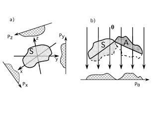
Figure 1: Schematic representation of different schemes for the experimental determination of the state of a quantum system S. (a) Quantum state tomography: a series of mutually incompatible measurements are performed, projecting the quantum state e.g. along the x, y, and z-axes. (b) The present approach: Part of the information in the quantum state is first transferred to the assistant A. A single measurement of the combined system S + A, in direction $\theta$, can then determine the complete initial state of S.

While these approaches all require a combination of measurements with incompatible observables, it is also possible to obtain the complete state information from a single measurement performed on a larger Hilbert space, provided the state information is first redistributed into this extended space D’Ariano (2002); Caves et al. (2002); Du et al. (2006); Allahverdyan et al. (2004). Ref. D’Ariano (2002) shows that it is possible to estimate the expectation values of all observables of a quantum system by measuring only a single “universal” observable on an extended Hilbert space. In the Hilbert space of the quantum system, the reduced operator of this “universal observable” constitutes a minimal informationally complete positive operator-valued measurement Caves et al. (2002). Du et al. Du et al. (2006) demonstrated an experimental example on this. Allahverdyan et al. Allahverdyan et al. (2004) determine the conditions for making this type of measurement robust by maximizing the determinant of the mapping between the quantum state and the measurement results.

The possibility of obtaining the full quantum state information from a single measurement appears highly attractive and may well have practical advantages since it avoids some experimental uncertainties related to measurement setups for incompatible observables. It requires, however, the redistribution of the information within the extended Hilbert space. This is achieved by coupling the system $S$, whose state is to be determined, to an assistant $A$ and letting the combined system evolve for a suitable period. The sketch of this measurement idea is shown in Fig. 1 b). As we show below, the success of the resulting measurements depends on the form of the Hamiltonian as well as on the duration of the evolution and the choice of the final measurement on the combined system.

In this paper, we study the details of this type of measurements using a (nuclear) spin 1/2 as the system whose quantum state is to be determined, and a different spin 1/2 as the assistant. We consider in detail what types of Hamiltonian can be used to couple the system to the assistant, how the information content of the resulting state can be maximized, and under what conditions the scheme will fail. As an experimental example, we present results from a nuclear spin system, using nuclear magnetic resonance (NMR).

II Coupling system and assistant

II.1 Hamiltonian

We consider two qubits interacting with local magnetic fields and coupled through the Heisenberg interaction. The system Hamiltonian can then be written as

$$\begin{array}[]{lll}\hat{H}&=&\hat{H}_{z}(B_{1},B_{2})+\hat{H}_{ex}(J_{x},J_{y},J_{z})\\ &=&B_{1}\hat{S}_{z}^{1}+B_{2}\hat{S}_{z}^{2}+\\ &&J_{x}\hat{S}_{x}^{1}\hat{S}_{x}^{2}+J_{y}\hat{S}_{y}^{1}\hat{S}_{y}^{2}+J_{z}\hat{S}_{z}^{1}\hat{S}_{z}^{2},\end{array}$$ (1)

where $\hat{S}_{\nu}^{k}=\frac{1}{2}\sigma_{\nu}^{k}(\nu=x,y,z)$ denotes the local spin operator for qubit $k$. The $B_{k}$s are the strengths of the external magnetic fields (along the z axis) acting on qubit $k$, and the $J_{\nu}$s are the Heisenberg exchange constants.

For arbitrary $J_{\nu}$, this is often called the anisotropic Heisenberg XYZ model. Some special cases are:

• XXX (or isotropic Heisenberg): $J_{x}=J_{y}=J_{z}$

• XXZ : $J_{x}=J_{y}\neq J_{z}$

• XY : $J_{z}=0$

• XZ : $J_{y}=0$

• Heisenberg-Ising : $J_{x}=J_{y}=0$

$J_{\nu}>0$ and $J_{\nu}<0$ correspond to the antiferromagnetic and ferromagnetic cases, respectively. In many solid-state systems, the coupling constants $J_{\nu}$ can be tuned by external fields and many proposals for solid-state quantum information processors rely on their tunability.

The Hamiltonian of Eq (1) splits into three mutually commuting parts,

$$\hat{H}=\hat{H}_{zz}+\hat{H}_{0}+\hat{H}_{2}$$ (2)

where

$$\begin{array}[]{l}\hat{H}_{zz}=J_{z}\hat{S}_{z}^{1}\hat{S}_{z}^{2}\\ \hat{H}_{0}=B\gamma_{B}(\hat{S}_{z}^{1}-\hat{S}_{z}^{2})+\frac{J}{2}(\hat{S}_{+}^{1}\hat{S}_{-}^{2}+\hat{S}_{-}^{1}\hat{S}_{+}^{2})\\ \hat{H}_{2}=B(\hat{S}_{z}^{1}+\hat{S}_{z}^{2})+\frac{J}{2}\gamma_{J}(\hat{S}_{+}^{1}\hat{S}_{+}^{2}+\hat{S}_{-}^{1}\hat{S}_{-}^{2}).\end{array}$$ (3)

$B=(B_{1}+B_{2})/2$ and $J=(J_{x}+J_{y})/2$ are the average field and the coupling constant, and $\gamma_{B}=(B_{1}-B_{2})/(B_{1}+B_{2})$ and $\gamma_{J}=(J_{x}-J_{y})/(J_{x}+J_{y})$ are anisotropy parameters. $\hat{S}_{\pm}^{k}=\hat{S}_{x}^{k}+i\hat{S}_{y}^{k}$ are the raising and lowering operators.

With this decomposition, the eigenvalues and eigenvectors can be easily calculated by diagonalizing the subspaces consisting of $\hat{H}_{0}$ and $\hat{H}_{2}$. We obtain for the eigenvalues

$$\begin{array}[]{l}\lambda_{1}=\frac{1}{4}J_{z}+\eta_{1},\\ \lambda_{2}=-\frac{1}{4}J_{z}+\eta_{2},\\ \lambda_{3}=-\frac{1}{4}J_{z}-\eta_{2},\\ \lambda_{4}=\frac{1}{4}J_{z}-\eta_{1},\end{array}$$ (4)

and for the eigenvectors

$$\begin{array}[]{cc}\left|\psi_{1}\right\rangle=\left(\begin{array}[]{c}\cos(\theta_{1}/2)\\ 0\\ 0\\ \sin(\theta_{1}/2)\end{array}\right)&\left|\psi_{2}\right\rangle=\left(\begin{array}[]{c}0\\ \cos\frac{\theta_{2}}{2}\\ \sin\frac{\theta_{2}}{2}\\ 0\end{array}\right)\\ \left|\psi_{3}\right\rangle=\left(\begin{array}[]{c}0\\ -\sin\frac{\theta_{2}}{2}\\ \cos\frac{\theta_{2}}{2}\\ 0\end{array}\right)&\left|\psi_{4}\right\rangle=\left(\begin{array}[]{c}-\sin(\theta_{1}/2)\\ 0\\ 0\\ \cos(\theta_{1}/2)\end{array}\right).\end{array}$$ (5)

Here

$$\begin{array}[]{l}\eta_{1}=\sqrt{B^{2}+(J\gamma_{J}/2)^{2}}\\ \eta_{2}=\sqrt{(B\gamma_{B})^{2}+(J/2)^{2}}\end{array}.$$ (6)

and

$$\begin{array}[]{l}\cos\frac{\theta_{1}}{2}=\sqrt{\frac{\eta_{1}+B}{2\eta_{1}}}\\ \sin\frac{\theta_{1}}{2}=\frac{J\gamma_{J}/2}{\sqrt{2\eta_{1}(\eta_{1}+B)}}=sgn(J\gamma_{J})\sqrt{\frac{\eta_{1}-B}{2\eta_{1}}}\\ \cos\frac{\theta_{2}}{2}=\sqrt{\frac{\eta_{2}+B\gamma_{B}}{2\eta_{2}}}\\ \sin\frac{\theta_{2}}{2}=\frac{J/2}{\sqrt{2\eta_{2}(\eta_{2}+B\gamma_{B})}}=sgn(J)\sqrt{\frac{\eta_{2}-B\gamma_{B}}{2\eta_{2}}}\end{array}.$$ (7)

II.2 Evolution

We write the evolution operator as a product of the evolutions generated by the three mutually commuting terms of Eq. (2):

$$\hat{U}(\tau)=e^{-i\hat{H}\tau}=\hat{U}_{zz}(\tau)\hat{U}_{0}(\tau)\hat{U}_{2}(\tau)$$ (8)

where

$$\begin{array}[]{lll}\hat{U}_{zz}(\tau)&=&e^{-i\hat{H}_{zz}\tau}\\ &=&\cos(\frac{J_{z}\tau}{4})\mathbf{1}-i\sin(\frac{J_{z}\tau}{4})(4\hat{S}^{1}_{z}\hat{S}^{2}_{z})\\ \hat{U}_{0}(\tau)&=&e^{-i\hat{H}_{0}\tau}\\ &=&\frac{1+\cos(\eta_{2}\tau)}{2}\mathbf{1}+\frac{1-\cos(\eta_{2}\tau)}{2}(4\hat{S}^{1}_{z}\hat{S}^{2}_{z})+\\ &&i2\cos\theta_{2}\sin(\eta_{2}\tau)(\hat{S}^{1}_{z}-\hat{S}^{2}_{z})+\\ &&i\sin\theta_{2}\sin(\eta_{2}\tau)(\hat{S}_{+}^{1}\hat{S}_{-}^{2}+\hat{S}_{-}^{1}\hat{S}_{+}^{2})\\ \hat{U}_{2}(\tau)&=&e^{-i\hat{H}_{2}\tau}\\ &=&\frac{1+\cos(\eta_{1}\tau)}{2}\mathbf{1}-\frac{1-\cos(\eta_{1}\tau)}{2}(4\hat{S}^{1}_{z}\hat{S}^{2}_{z})+\\ &&i2\cos\theta_{1}\sin(\eta_{1}\tau)(\hat{S}^{1}_{z}+\hat{S}^{2}_{z})+\\ &&i\sin\theta_{1}\sin(\eta_{1}\tau)(\hat{S}_{+}^{1}\hat{S}_{+}^{2}+\hat{S}_{-}^{1}\hat{S}_{-}^{2}).\\ \end{array}$$ (9)

In the following, we will use a different operator basis for the diagonal terms: we define the polarization operators $I_{i}^{\alpha,\beta}=\frac{1}{2}\mathbf{1}\pm\hat{S}_{z}^{(i)}$. In terms of these operators, the total propagator becomes

$$\hat{U}(\tau)=a_{1}I_{1}^{\alpha}I_{2}^{\alpha}+a_{2}I_{1}^{\alpha}I_{2}^{\beta}+a_{3}I_{1}^{\beta}I_{2}^{\alpha}+a_{4}I_{1}^{\beta}I_{2}^{\beta}$$

$$+d(\hat{S}_{+}^{1}\hat{S}_{-}^{2}+\hat{S}_{-}^{1}\hat{S}_{+}^{2})+b(\hat{S}_{+}^{1}\hat{S}_{+}^{2}+\hat{S}_{-}^{1}\hat{S}_{-}^{2}),$$ (10)

where

$$\begin{array}[]{l}a_{1}=\cos^{2}\frac{\theta_{1}}{2}e^{-i\lambda_{1}\tau}+\sin^{2}\frac{\theta_{1}}{2}e^{-i\lambda_{4}\tau}\\ a_{2}=\cos^{2}\frac{\theta_{2}}{2}e^{-i\lambda_{2}\tau}+\sin^{2}\frac{\theta_{2}}{2}e^{-i\lambda_{3}\tau}\\ a_{3}=\sin^{2}\frac{\theta_{2}}{2}e^{-i\lambda_{2}\tau}+\cos^{2}\frac{\theta_{2}}{2}e^{-i\lambda_{3}\tau}\\ a_{4}=\sin^{2}\frac{\theta_{1}}{2}e^{-i\lambda_{1}\tau}+\cos^{2}\frac{\theta_{1}}{2}e^{-i\lambda_{4}\tau}\\ b=\frac{1}{2}\sin\theta_{1}(e^{-i\lambda_{1}\tau}-e^{-i\lambda_{4}\tau})\\ d=\frac{1}{2}\sin\theta_{2}(e^{-i\lambda_{2}\tau}-e^{-i\lambda_{3}\tau}).\end{array}$$ (11)

As we show in the following section, the evolution of Eq. (8) transfers information between qubits in such a way that it becomes possible to measure the complete quantum state of one qubit with a single apparatus, as proposed by Allahverdyan et al.Allahverdyan et al. (2004).

III Measurement procedure

III.1 Principle

Consider a two-level system S (spin-$\frac{1}{2}$) whose state can be represented by $\hat{\rho}=\left(\begin{array}[]{cc}\rho_{11}&\rho_{12}\\ \rho_{21}&\rho_{22}\\ \end{array}\right)$ with the normalization $\rho_{11}+\rho_{22}=1$. To determine the state $\hat{\rho}$, we can measure the vector $\vec{s}=2Tr(\vec{\hat{S}}\hat{\rho})=(s_{x},s_{y},s_{z})^{T}$ where $s_{x}=\rho_{12}+\rho_{21}$, $s_{y}=i(\rho_{12}-\rho_{21})$, $s_{z}=\rho_{11}-\rho_{22}$ and $\vec{\hat{S}}=(\hat{S}_{x},\hat{S}_{y},\hat{S}_{z})^{T}$.

To transfer part of the state information to the assistant $A$, we couple the two subsystems with the interaction Hamiltonian $\hat{H}$ of Eq.(1). At the time $t=0$, the composite system S+A is in the state $\hat{\varrho}_{0}=\hat{\rho}^{(S)}\otimes\hat{\xi}^{(A)}$. Without loss of generality, we assume $\hat{\xi}=\frac{1}{2}\mathbf{1}+\epsilon S_{z},(0\leq\epsilon\leq 1)$. Here, the superscripts $S$ and $A$ refer to the two subsystems.

Under the effect of the coupling Hamiltonian of Eq. (1), this state evolves into $\hat{\varrho}_{\tau}=\hat{U}(\tau)\,\hat{\varrho}_{0}\,\hat{U}^{{\dagger}}(\tau)$. On this state, we perform repeatedly measure the simplest possible nondegenerate, factorized observable $\hat{\Omega}=\sum_{\alpha=1}^{4}\varpi_{\alpha}\hat{P}_{\alpha}$, which determines the complete set $\{P_{\alpha}\}$ of the joint probabilities, They correspond to the eigenvalues of $\hat{\varrho}_{\tau}$ in the eigenbasis of the observable $\hat{\Omega}$. Since these values were generated from the initial state by a one-to-one mapping, $P_{\alpha}=P_{kq}=\sum_{ij}\mathcal{M}_{kq,ij}\rho_{ij}$, we can invert this mapping to calculate the original state $\hat{\rho}$ Allahverdyan et al. (2004).

The precision of the back-calculation depends on the size of the determinant $\Delta=\det(M_{kq,ij})$: If $|\Delta|$ is small, any (experimental) error in the measurement of $P_{kq}$ will result in a large error in $\rho_{ij}$, roughly $\propto 1/|\Delta|$. We therefore seek to maximize $|\Delta|$ and thereby the precision of the measurement. This maximization is achieved by a suitable choice of the Hamiltonian $\hat{H}$, the duration $\tau$, and the single observable $\hat{\Omega}$.

III.2 Symmetry properties of the evolution

The Hamiltonian $\hat{H}$ of Eq. (1) consists of three commuting parts: $\hat{H}_{zz}$, $\hat{H}_{0}$, and $\hat{H}_{2}$. All of these terms are invariant under $\pi$-rotations around the z-axis. We use this property to separate the density operator into two parts that transform irreducibly under this symmetry operation: One part which is invariant with respect to $\pi_{z}$ rotations, and the second part, which changes sign. The first part includes diagonal terms, zero quantum and double quantum coherence Ernst et al. (1994); the second part includes the single quantum coherence terms. The symmetry of the Hamiltonian implies that the evolution does not transfer information from one subspace to the other. Figure 2 illustrates the division of the density operator into these subspaces.

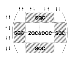
Figure 2: Subspaces of the density operator that are invariant by the evolution under the Hamiltonian of Eq. (1).

A consequence of this separation of the system into two distinct subspaces is that it restricts the possible choice of observables. In particular, if we choose the z-components of the two spins to the single observable $\hat{\Omega}$, then all possible combinations fall into the subspace that is invariant under $\pi_{z}$ rotations and therefore does not provide information about the other subspace. For this paper, we choose the x-components of both spins; another, equivalent choice would be the y-components.

III.3 Transfer matrix

This evolution process, together with the subsequent measurement of the single observable $\hat{\Omega}$, transfers the information from the initial state $\hat{\varrho}_{0}$ to the set of measurement results $P_{\alpha}=P_{kq}$, which are the expectation values of the operators

$$\hat{P}_{kq}=(\frac{1}{2}\mathbf{1}-(-1)^{k}\hat{S}_{x}^{(S)})\otimes(\frac{1}{2}\mathbf{1}-(-1)^{q}\hat{S}_{x}^{(A)})$$

acting on the state $\hat{\varrho}_{\tau}$:

$$P_{kq}=Tr\{\hat{P}_{kq}\hat{U}(\tau)\hat{\varrho}_{0}\hat{U}^{\dagger}(\tau)\}.$$

The indices $k,q$ can have the values 1, 2.

We use the transfer matrix $\mathcal{M}$ to describe this map:

$$\mathcal{M}\left(\begin{array}[]{c}\rho_{11}\\ \rho_{12}\\ \rho_{21}\\ \rho_{22}\end{array}\right)=\left(\begin{array}[]{c}P_{11}\\ P_{12}\\ P_{21}\\ P_{22}\end{array}\right).$$ (12)

Its elements are

$$\begin{array}[]{l}\mathcal{M}_{11,11}=\mathcal{M}_{22,11}=\frac{1}{8}((1+\epsilon)|a_{1}+b|^{2}+(1-\epsilon)|a_{2}+d|^{2})\\ \mathcal{M}_{12,11}=\mathcal{M}_{21,11}=\frac{1}{8}((1+\epsilon)|a_{1}-b|^{2}+(1-\epsilon)|a_{2}-d|^{2})\\ \mathcal{M}_{11,12}=-\mathcal{M}_{22,12}=\mathcal{M}_{11,21}^{*}=-\mathcal{M}_{22,21}^{*}\\ =\frac{1}{8}((1+\epsilon)(a_{1}+b)(a_{3}^{*}+d^{*})+(1-\epsilon)(a_{2}+d)(a_{4}^{*}+b^{*})\\ \mathcal{M}_{22,22}=-\mathcal{M}_{21,12}=\mathcal{M}_{12,21}^{*}=-\mathcal{M}_{33}^{*}\\ =\frac{1}{8}((1+\epsilon)(a_{1}-b)(a_{3}^{*}-d^{*})+(1-\epsilon)(a_{2}-d)(a_{4}^{*}-b^{*})\\ \mathcal{M}_{11,22}=\mathcal{M}_{22,22}=\frac{1}{8}((1+\epsilon)|a_{3}+d|^{2}+(1-\epsilon)|a_{4}+b|^{2})\\ \mathcal{M}_{12,22}=\mathcal{M}_{21,22}=\frac{1}{8}((1+\epsilon)|a_{3}-d|^{2}+(1-\epsilon)|a_{4}-b|^{2})\\ \end{array}$$ (13)

and its determinant is

$$\Delta=8\Im(\mathcal{M}_{12,12}^{*}\mathcal{M}_{11,12})(\mathcal{M}_{11,11}\mathcal{M}_{12,22}-\mathcal{M}_{12,11}\mathcal{M}_{11,22}).$$ (14)

Here $\Im(c)$ denotes the imaginary part of $c$. Using Eqs. (4), (7), (11) and (13), we find for its absolute value

$$\begin{array}[]{ll}|\Delta|=&\frac{1}{32}|(1-\epsilon^{2})\sin(-J_{z}\tau)\{[\sin(2\theta_{1})\sin^{2}(\eta_{1}\tau)]^{2}-\\ &[\sin(2\theta_{2})\sin^{2}(\eta_{2}\tau)]^{2}\}+2\epsilon[\sin(2\theta_{1})\sin^{2}(\eta_{1}\tau)\\ &+\sin(2\theta_{2})\sin^{2}(\eta_{2}\tau)]\{[1-2\sin^{2}\theta_{1}\sin^{2}(\eta_{1}\tau)]\\ &\times\sin\theta_{2}\sin(2\eta_{2}\tau)-[1-2\sin^{2}\theta_{2}\sin^{2}(\eta_{2}\tau)]\\ &\times\sin\theta_{1}\sin(2\eta_{1}\tau)\}|.\end{array}$$ (15)

IV Optimization: Maximizing $|\Delta|$

The size of the determinant $|\Delta|$ of the transfer mapping determines the quality of measurement. Maximizing $|\Delta|$ will minimize the statistical error of the estimation during the inversion of Eq. (12). We can maximize it by an appropriate choice of the initial condition of the assistant, the parameters of the Hamiltonian that generates the evolution $U$, and the duration of the evolution.

Figure 3 plots the maximum possible determinant size $|\Delta|_{max}$ for the Hamiltonian of Eq. (1) as a function of the polarization $\epsilon$ of the assistant. Clearly, the quality of the measurement should increase with increasing polarization of the assistant. The dashed line in Fig. 3 shows for comparison the maximum possible value for a general exchange interaction, taken from Ref. Allahverdyan et al. (2004). At the extreme cases of zero and full polarization, the Heisenberg coupling Hamiltonian allows one to reach the maximum possible value, but for intermediate polarizations, its maximum value is slightly lower than for the general case.

Let us now focus on two extreme situations $\epsilon=1$ (a pure state) and $\epsilon=0$ (a completely disordered state).

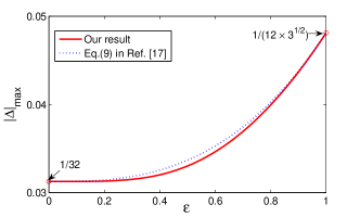
Figure 3: (Color Online) Maximal determinant size $|\Delta|_{max}$ versus the polarization $\epsilon$ by the Heisenberg exchange interaction (1), compared to the general case of arbitrary exchange interaction (Eq. (9)) in Ref. Allahverdyan et al. (2004)).

IV.1 Assistant in pure state

When the assistant A starts in a pure state $\hat{\xi}^{(A)}=\frac{1}{2}\mathbf{1}+S_{z}^{(A)}$ (corresponding to $\epsilon=1$), the determinant becomes

$$\begin{array}[]{ll}|\Delta|=&\frac{1}{16}|[\sin(2\theta_{1})\sin^{2}(\eta_{1}\tau)+\sin(2\theta_{2})\sin^{2}(\eta_{2}\tau)]\\ &\times\{[1-2\sin^{2}\theta_{1}\sin^{2}(\eta_{1}\tau)]\sin\theta_{2}\sin(2\eta_{2}\tau)\\ &-[1-2\sin^{2}\theta_{2}\sin^{2}(\eta_{2}\tau)]\sin\theta_{1}\sin(2\eta_{1}\tau)\}|.\end{array}$$ (16)

We can see from this expression that $|\Delta|$ is independent of the coupling strength $J_{z}$ along the z-axis. A Heisenberg XY interaction is therefore sufficient for optimizing the evolution. We therefore specialize to this case. Using the substitutions

$$\begin{array}[]{l}\sin\frac{\Xi_{k}}{2}=\sin\theta_{k}\sin(\eta_{k}\tau)\\ \sin\Lambda_{k}=\cos(\eta_{k}\tau)/\cos\frac{\Xi_{k}}{2},(k=1,2),\end{array}$$ (17)

we rewrite $|\Delta|$ as

$$\begin{array}[]{ll}|\Delta|=&\frac{1}{16}|(\sin\Xi_{1}\cos\Lambda_{1}+\sin\Xi_{2}\cos\Lambda_{2})\\ &\times(\cos\Xi_{1}\sin\Xi_{2}\sin\Lambda_{2}-\cos\Xi_{2}\sin\Xi_{1}\sin\Lambda_{1})|.\end{array}$$ (18)

In terms of these parameters, an optimal solution ($|\Delta|=1/(12\sqrt{3})$) is given by the following set of parameters:

$$\begin{array}[]{l}\Lambda_{1}=\Lambda_{2}=\Lambda\\ \sin(2\Lambda)=\pm 1\\ \sin\frac{\Xi_{1}-\Xi_{2}}{2}=\pm\frac{1}{\sqrt{3}}\\ \sin\frac{\Xi_{1}+\Xi_{2}}{2}=\pm 1.\end{array}$$ (19)

This parameter set corresponds to the following parameters of the Hamiltonian (1):

$$\begin{array}[]{l}\eta_{k}\tau=m\pi\pm\frac{1}{2}\arccos(-\Gamma_{k})\\ B=\pm\eta_{1}\sqrt{(1-\Gamma_{1})/(1+\Gamma_{1})}\\ \gamma_{B}=\pm\sqrt{\frac{(1+\Gamma_{1})(1-\Gamma_{2})}{(1-\Gamma_{1})(1+\Gamma_{2})}}\frac{\eta_{2}}{\eta_{1}}\\ J=\pm 4\eta_{2}\sqrt{2\Gamma_{2}/(1+\Gamma_{2})}\\ \gamma_{J}=\pm\sqrt{\frac{\Gamma_{1}(1+\Gamma_{2})}{\Gamma_{2}(1+\Gamma_{1})}}\frac{\eta_{1}}{\eta_{2}}.\end{array}$$ (20)

Here, $m$ is an integer and $\Gamma_{k}=\sin^{2}\frac{\Xi_{k}}{2},(k=1,2)$. $(\Gamma_{1},\Gamma_{2})$ take the pairs of values $(\frac{1}{2}-\frac{\sqrt{3}}{6},\frac{1}{2}+\frac{\sqrt{3}}{6})$ or $(\frac{1}{2}+\frac{\sqrt{3}}{6},\frac{1}{2}-\frac{\sqrt{3}}{6})$. Without loss of generality, we set $\tau=1$. The optimal Hamiltonian is then

$$H^{opt}=1.1458\hat{S}_{z}^{1}-0.2935\hat{S}_{z}^{2}+3.3820\hat{S}_{x}^{1}\hat{S}_{x}^{2}-1.2747\hat{S}_{y}^{1}\hat{S}_{y}^{2}.$$ (21)

IV.2 Completely disordered assistant.

When the assistant A is initially in a completely disordered state $\hat{\xi}^{(A)}=\frac{1}{2}\mathbf{1}$ ($\epsilon=0$), we have

$$\begin{array}[]{ll}|\Delta|=&\frac{1}{32}|\sin(-J_{z}\tau)||\{[(\sin(2\theta_{1})\sin^{2}(\eta_{1}\tau)]^{2}\\ &-[(\sin(2\theta_{2})\sin^{2}(\eta_{2}\tau)]^{2}\}|.\end{array}$$ (22)

$|\Delta|$ reaches its maximum of $1/32$ when

$$\sin(J_{z}\tau)=\pm 1\Rightarrow J_{z}\tau=\frac{\pi}{2}(2n-1)$$ (23)

($n$ integer) and simultaneously

$$\sin(2\theta_{1})\sin^{2}(\eta_{1}\tau)=\pm 1\mbox{ and }\sin(2\theta_{2})\sin^{2}(\eta_{2}\tau)=0$$ (24)

or

$$\sin(2\theta_{1})\sin^{2}(\eta_{1}\tau)=0\mbox{ and }\sin(2\theta_{2})\sin^{2}(\eta_{2}\tau)=\pm 1.$$ (25)

Condition (24) corresponds to the following parameters for the Hamiltonian:

$$\begin{array}[]{ccl}|B|\tau&=&|2m-1|\frac{\sqrt{2}\pi}{4}\\ |J_{x}-J_{y}|&=&4|B|\\ \gamma_{B}&=&0\mbox{ OR }J_{x}+J_{y}=0\mbox{ OR }\eta_{2}\tau=l\pi\\ \end{array}$$ (26)

and (25) to

$$\begin{array}[]{ccl}|J|\tau&=&|2m-1|\frac{\sqrt{2}\pi}{2}\\ |B_{1}-B_{2}|&=&|J|\\ B_{1}+B_{2}&=&0\mbox{ OR }\gamma_{J}=0\mbox{ OR }\eta_{1}\tau=l\pi,\end{array}$$ (27)

where $m,l$ are integers.

These relationships define six classes of Heisenberg exchange interactions that optimally transfer information from the system to the combined system plus assistant. The transfer is determined by the product of the Hamiltonian and the evolution time $\tau$. Without loss of generality, we choose $\tau=\frac{\pi}{4}$. In these units, some possibilities are

(a)

XYX model: $H^{opt}=\sqrt{2}(\hat{S}_{z}^{1}+\hat{S}_{z}^{2})+2(\hat{S}_{x}^{1}\hat{S}_{x}^{2}+\hat{S}_{z}^{1}\hat{S}_{z}^{2})+2(1-2\sqrt{2})\hat{S}_{y}^{1}\hat{S}_{y}^{2}$, as shown in Ref.Allahverdyan et al. (2004);

(b)

XXZ model: $H^{opt}=\sqrt{2}(\hat{S}_{z}^{1}-\hat{S}_{z}^{2})+2\sqrt{2}(\hat{S}_{x}^{1}\hat{S}_{x}^{2}+\hat{S}_{y}^{1}\hat{S}_{y}^{2})+2\hat{S}_{z}^{1}\hat{S}_{z}^{2}$;

(c)

XZ model: $H^{opt}=\sqrt{2}(\hat{S}_{z}^{1}\pm\hat{S}_{z}^{2})+4\sqrt{2}\hat{S}_{x}^{1}\hat{S}_{x}^{2}+2\hat{S}_{z}^{1}\hat{S}_{z}^{2}$.

V Failure analysis

The measurement scheme fails when $\Delta=0$. From Eq. (15), we see that this occurs when

$$\sin(2\theta_{1})\sin^{2}(\eta_{1}\tau)+\sin(2\theta_{2})\sin^{2}(\eta_{2}\tau)=0$$ (28)

or when

$$\begin{array}[]{l}(1-\epsilon^{2})\sin(-J_{z}\tau)[\sin(2\theta_{1})\sin^{2}(\eta_{1}\tau)-\sin(2\theta_{2})\sin^{2}(\eta_{2}\tau)]\\ +2\epsilon\{[1-2\sin^{2}\theta_{1}\sin^{2}(\eta_{1}\tau)]\sin\theta_{2}\sin(2\eta_{2}\tau)\\ -[1-2\sin^{2}\theta_{2}\sin^{2}(\eta_{2}\tau)]\sin\theta_{1}\sin(2\eta_{1}\tau)\}=0,\end{array},$$ (29)

independent of the initial state of the assistant A.

A simple case is $\sin(2\theta_{1})=\sin(2\theta_{2})=0$, i.e., $J=0$ or $B=0$ or ($\gamma_{B}=0$ and $\gamma_{J}=0$). These cases correspond, e.g., to

• a weakly-coupled liquid-state NMR Hamiltonian ($J_{x}=J_{y}=0$)

• any Heisenberg interaction without external field

• an isotropic Heisenberg interaction in the XY plane in a uniform external field.

In all of these cases, the resulting evolution cannot generate a state that allows one to measure the complete information.

Another case that fulfills Eq. (28) is

$$\sin(2\theta_{1})=-\sin(2\theta_{2})\Rightarrow\frac{\gamma_{J}}{\gamma_{B}}=-\frac{\eta_{1}^{2}}{\eta_{2}^{2}}$$ (30)

and

$$|\sin(\eta_{1}\tau)|=|\sin(\eta_{2}\tau)|\Rightarrow\eta_{1}\tau=|m\pi\pm\eta_{2}\tau|.$$ (31)

If, e.g., $\eta_{1}=\eta_{2}$, we get the condition

$$(\gamma_{B},\gamma_{J})=(1,\pm 1)\mbox{ or }(-1,1)$$ (32)

for $\Delta=0$.

From Eq. (15), we can seen that for $\epsilon=1$ (a pure state), $|\Delta|$ does not depend on $J_{z}$, while for $\epsilon=0$ (completely disordered state), $|\Delta|$ depends strongly on $J_{z}$. For $\epsilon=0$, it is obvious that $\Delta=0$ when

$$\sin(J_{z}\tau)=0\Rightarrow J_{z}\tau=n\pi.$$ (33)

Hence, the existence of the coupling along the z-axis (i.e.,$J_{z}\neq 0$) is a necessary condition for this measurement scheme when the assistant A is initially prepared in a completely disordered state. In this case, the failure condition (32) can be further modified to

$$(\gamma_{B},\gamma_{J})=(\pm 1,\pm 1),$$ (34)

which means that when any two among $J_{x},J_{y},B_{1},B_{2}$ are equal to zero, the measurement scheme fails.

VI Quantum Simulation of the Exchange Hamiltonian

In liquid-state NMR systems, the natural Hamiltonian for a system of two spins is

$$\hat{H}_{NMR}=\omega_{1}\hat{S}_{z}^{1}+\omega_{2}\hat{S}_{z}^{2}+2\pi J_{12}\hat{S}_{z}^{1}\hat{S}_{z}^{2},$$ (35)

where $\omega_{1,2}$ represent the Larmor angular frequencies of the two qubits (in the rotating frame) and $J_{12}$ the spin-spin coupling constant. This is equivalent to the Heisenberg-Ising model. As discussed in the preceding section, this Hamiltonian cannot be used to transfer the information, since the transfer matrix becomes singular, $\Delta\equiv 0$. Therefore, the key to implement this measurement scheme in a liquid-state NMR system is to first perform a quantum simulation of the Hamiltonian (1). We briefly discuss two techniques for realizing such an evolution.

VI.1 Short period expansion

Assuming that we can realize parts of the Hamiltonian experimentally, we write the total Hamiltonian as a sum,

$$\hat{H}=\sum\limits_{k=1}^{L}\hat{H}_{k}.$$

In general, the different terms do not commute with each other, and it is therefore not sufficient to generate them sequentially. However, if the evolution under each term is sufficiently short, it is possible to approximate the overall evolution in this way.

Using a symmetrized version of the Trotter formula Trotter (1959),

$$e^{(A+B)\tau}=e^{(A\tau/2)}e^{(B\tau)}e^{(A\tau/2)}+O(\tau^{3})$$

we expand the propagator as

$$e^{-i\hat{H}\Delta t}\simeq[e^{-i\hat{H}_{1}\frac{\Delta t}{2}}e^{-i\hat{H}_{2}\frac{\Delta t}{2}}...e^{-i\hat{H}_{L}\frac{\Delta t}{2}}]$$

$$\cdot[e^{-i\hat{H}_{L}\frac{\Delta t}{2}}e^{-i\hat{H}_{L-1}\frac{\Delta t}{2}}...e^{-i\hat{H}_{1}\frac{\Delta t}{2}}]+O(\Delta t^{3}),$$ (36)

which approximates the desired evolution to second order in $\Delta t$. Keeping $\Delta t$ short enough, this allows one to efficiently simulate the target Hamiltonian (1) by concatenating these evolution periods until the correct total evolution is reached.

Our target Hamiltonian can be decomposed into two non-commuting parts $\hat{H}_{z}+\hat{H}_{zz}$ and $\hat{H}_{xy}=J_{x}\hat{S}^{1}_{x}\hat{S}^{2}_{x}+J_{y}\hat{S}^{1}_{y}\hat{S}^{2}_{y}$. We thus generate the overall evolution (8) as

$$\hat{U}(\tau)=\hat{U}^{m}(\Delta t)=[\hat{U}_{z}(\frac{\Delta t}{2})\hat{U}_{xy}(\Delta t)\hat{U}_{z}(\frac{\Delta t}{2})]^{m}+O(\Delta t^{3}),$$ (37)

where $\tau=m\Delta t$ is the total duration, and

$$\hat{U}_{z}(\frac{\Delta t}{2})=e^{-i(\hat{H}_{z}+\hat{H}_{zz})\frac{\Delta t}{2}},$$

and

$$\hat{U}_{xy}(\Delta t)=e^{-i\hat{H}_{xy}\Delta t}$$

represent the evolutions under the partial Hamiltonians.

Taking as an example the XZ model (case (c) in Sec. IV B), it is sufficient to choose the number of evolution periods $m=2$ for $\tau=\pi/4$: the resulting approximate evolution

$$\hat{U}^{ap}(\tau)=[\hat{U}_{z}(\frac{\pi}{16})\hat{U}_{xy}(\frac{\pi}{8})\hat{U}_{z}(\frac{\pi}{16})]^{2}$$

with

$$\hat{U}_{z}(\frac{\pi}{16})=e^{-i[(\sqrt{2}(\hat{S}^{1}_{z}\pm\hat{S}^{2}_{z})+2\hat{S}^{1}_{z}\hat{S}^{2}_{z}]\frac{\pi}{16}}$$

and

$$\hat{U}_{xy}(\frac{\pi}{8}) = e^{-i\hat{S}^{1}_{x}\hat{S}^{2}_{x}\frac{\sqrt{2}\pi}{2}}$$ (38)

$$= e^{-i(\hat{S}^{1}_{y}+\hat{S}^{2}_{y})\frac{\pi}{2}}e^{-i\hat{S}^{1}_{z}\hat{S}^{2}_{z}\frac{\sqrt{2}\pi}{2}}e^{i(\hat{S}^{1}_{y}+\hat{S}^{2}_{y})\frac{\pi}{2}}$$

has a fidelity of 0.9958 with the target evolution, where the fidelity is defined as

$$F(\hat{U}(\tau),\hat{U}^{ap}(\tau))=\frac{Tr(\hat{U}^{{\dagger}}(\tau)\hat{U}^{ap}(\tau))}{4}.$$

The $\hat{U}_{z}(\frac{\pi}{16})$ operator can be implemented by a free evolution period under the internal Hamiltonian if we choose $\omega_{1}=\pm\omega_{2}=\sqrt{2}\pi J_{12}$ and set the duration to $d_{1}=\frac{1}{16\,J_{12}}$.

The $\hat{U}_{xy}(\frac{\pi}{8})$ operator can be implemented by four $\frac{\pi}{2}$ pulses (corresponding to $e^{-i\hat{S}^{i}_{y}\frac{\pi}{2}}$) and a free precession period of duration $d_{2}=\frac{\sqrt{2}}{4J_{12}}$. This evolution period implements $e^{-i\hat{S}^{1}_{z}\hat{S}^{2}_{z}\frac{\sqrt{2}\pi}{2}}$; we therefore refocus the chemical shift terms by inserting refocusing $\pi$ pulses in the middle of this period. According to Eq. (38), the second set of $\pi/2$ pulses should rotate the spins around the $-y$ axis. Here, we choose the $+y$-axis instead to compensate for the inversion of the axes system by the $\pi$-pulses.

The resulting pulse sequence that generates one segment of $\hat{U}^{ap}(\tau)$ is

$$d_{1}-\left[\frac{\pi}{2}\right]_{y}^{1}\left[\frac{\pi}{2}\right]_{y}^{2}-\frac{d_{2}}{2}-\left[\pi\right]_{-y}^{1}\left[\pi\right]_{-y}^{2}-\frac{d_{2}}{2}-\left[\frac{\pi}{2}\right]_{y}^{1}\left[\frac{\pi}{2}\right]_{y}^{2}-d_{1},$$ (39)

where $\left[\theta\right]_{\hat{\nu}}^{k}$ denotes a $\theta$ rotation of qubit $k$ around the $\hat{\nu}$ axis.

VI.2 Exact decomposition

In some cases, it is possible to achieve the exact transformation by a suitable decomposition of the evolution, using, e.g.,

$$e^{-i\hat{R}\hat{H}\hat{R}^{{\dagger}}\tau}=\hat{R}e^{-i\hat{H}\tau}\hat{R}^{{\dagger}}.$$

For the propagator (8), we can use the decomposition

$$\hat{U}=\hat{R}\cdot e^{-i\hat{H}_{diag}\tau}\cdot\hat{R}^{\dagger},$$ (40)

where $\hat{H}_{diag}$ is the diagonal form of the Hamiltonian. The transformation

$$\hat{R}=\left(\begin{array}[]{llll}\cos\frac{\theta_{1}}{2}&&&-\sin\frac{\theta_{1}}{2}\\ &\cos\frac{\theta_{2}}{2}&-\sin\frac{\theta_{2}}{2}\\ &\sin\frac{\theta_{2}}{2}&\cos\frac{\theta_{2}}{2}\\ \sin\frac{\theta_{1}}{2}&&&\cos\frac{\theta_{1}}{2}\end{array}\right),$$ (41)

which diagonalizes the Hamiltonian (1), can be implemented experimentally (up to an irrelevant overall phase factor) by the pulse sequence

$$\left[\frac{\pi}{2}\right]_{-y}^{1}\left[\frac{\pi}{2}\right]_{\varphi}^{2}-\frac{\tau_{1}}{2}-\left[\pi\right]_{y}^{1}\left[\pi\right]_{-x}^{2}-\frac{\tau_{1}}{2}-\left[\frac{\pi}{2}\right]_{-x}^{1}\left[\frac{\pi}{2}\right]_{y}^{2}$$

$$-\frac{\tau_{2}}{2}-\left[\pi\right]_{x}^{1}\left[\pi\right]_{-y}^{2}-\frac{\tau_{2}}{2}-\left[\frac{\pi}{2}\right]_{-x}^{1}\left[\frac{\pi}{2}\right]_{-y}^{1}\left[\frac{\pi}{2}\right]_{y}^{2}\left[\frac{\pi}{2}\right]_{\varphi}^{2}$$

(42)

with $\tau_{1}=\frac{2|\theta_{1}-\theta_{2}|}{\pi J_{12}}$, $\tau_{2}=\frac{2|\theta_{1}+\theta_{2}|}{\pi J_{12}}$ and $\varphi=x$ or $-x$ for $\theta_{1}>\theta_{2}$ or $\theta_{1}<\theta_{2}$, and $\hat{R}^{\dagger}$ by the Hermite time-reversed sequence.

The evolution under the diagonal Hamiltonian

$$\begin{array}[]{l}\hat{U}_{diag}=e^{-i\hat{H}_{diag}\tau}=\left(\begin{array}[]{llll}e^{-i\lambda_{1}\tau}\\ &e^{-i\lambda_{2}\tau}\\ &&e^{-i\lambda_{3}\tau}\\ &&&e^{-i\lambda_{4}\tau}\end{array}\right)\\ \end{array}$$ (43)

is realized by the pulse sequence

$$\frac{\tau_{3}}{2}-\left[\pi\right]_{x}^{1}\left[\pi\right]_{x}^{2}-\frac{\tau_{3}}{2}-\left[\frac{\pi}{2}\right]_{-x}^{1}\left[\frac{\pi}{2}\right]_{-x}^{2}\left[\beta_{1}\right]_{y}^{1}\left[\beta_{2}\right]_{y}^{2}\left[\frac{\pi}{2}\right]_{-x}^{1}\left[\frac{\pi}{2}\right]_{-x}^{2},$$ (44)

where $\tau_{3}=\frac{\lambda_{1}-\lambda_{2}-\lambda_{3}+\lambda_{4}}{2\pi J_{12}}\tau$, $\beta_{1}=\frac{\lambda_{1}+\lambda_{2}-\lambda_{3}-\lambda_{4}}{2}\tau$ and $\beta_{2}=\frac{\lambda_{1}-\lambda_{2}+\lambda_{3}-\lambda_{4}}{2}\tau$. The first part of this sequence implements an evolution under the J-coupling alone, the second part implements a composite $z-$rotation of the two qubits by angles $\beta_{1}$ and $\beta_{2}$.

An alternative realization of $\hat{U}_{diag}$ is achieved by letting the system evolve under a constant Hamiltonian with

$$\omega_{1}=\frac{\lambda_{1}+\lambda_{2}-\lambda_{3}-\lambda_{4}}{2}\cdot\frac{\tau}{\tau_{3}}$$

and

$$\omega_{2}=\frac{\lambda_{1}-\lambda_{2}+\lambda_{3}-\lambda_{4}}{2}\cdot\frac{\tau}{\tau_{3}}$$

for a period $\tau_{3}$.

For the example (c) in Sec. IV B, we choose the parameters

$$\tau_{1} = \tau_{3}=\frac{1}{4J_{12}},\tau_{2}=\frac{3}{4J_{12}},$$

$$\beta_{1} = \frac{\pi(2+\sqrt{2})}{4},\beta_{2}=\frac{\pi(2-\sqrt{2})}{4}.$$ (45)

When $B_{1}=B_{2}$, $\varphi=x$ in the sequence (42); when $B_{1}=-B_{2}$, $\varphi=-x$.

VII EXPERIMENTAL IMPLEMENTATION

Experiments were performed at room temperature on a Bruker Avance II 500 MHz spectrometer equipped with a Triple-Broadband-Observe(TBO) probe at the frequencies 500.23 MHz for ¹H and 125.13 MHz for ¹³C. For the qubit system, we chose ¹³C-labelled chloroform diluted in acetone-d₆. The “unknown” state $\hat{\rho}$ was prepared on the spin of the proton nuclei (¹H), which served as the quantum system S (qubit 1), and the spin of the ¹³C nuclei was taken as the assistant A (qubit 2). The spin-spin coupling constant is $J_{12}=214.95Hz$. The relaxation times were $T_{1}=16.5$ s and $T_{2}=6.9$ s for the proton, and $T_{1}=21.2$ s and $T_{2}=0.35$ s for the carbon nuclei.

VII.1 Experimental procedure

There are three steps to implement the measurement scheme stated above: (i) Preparation of the initial system, (ii) Quantum simulation and (iii) Measurement.

Any qubit state $\hat{\rho}=\frac{1}{2}\mathbf{1}+\vec{s}\cdot\vec{\hat{S}}$ can be parameterized as a vector in the Bloch sphere:

$$\vec{s}(r,\theta,\phi) = (s_{x},s_{y},s_{z})^{T}$$ (46)

$$= \left(r\sin\theta\cos\phi,r\sin\theta\cos\phi,r\cos\theta\right)^{T},$$

where the amplitude $r=1$ for a pure state, and $0\leq r<1$ for mixed states and $\theta$, and $\phi$ are, respectively, the polar and azimuthal angles.

The combined system was initialized in the state $\hat{\varrho}_{0}=\hat{\rho}^{\left(S\right)}\otimes\hat{\xi}^{\left(A\right)}$. In our demonstration experiment we chose a completely disordered state $\hat{\xi}=\frac{1}{2}\mathbf{1}^{\left(A\right)}$ that is experimentally easy to prepare. Such an initial state $\hat{\varrho}_{0}=\hat{\rho}^{\left(S\right)}\otimes\frac{1}{2}\mathbf{1}^{\left(A\right)}$ was prepared by the NMR pulse sequence:

$$\left[\arccos\left(r\right)\right]_{y}^{1}\left[\frac{\pi}{2}\right]_{y}^{2}-G_{z}-\left[\theta\right]_{\phi+\pi/2}^{1}.$$ (47)

The first two RF pulses define the amount of spin polarization on the two qubits. The field gradient pulse $G_{z}$ dephases transverse magnetization to eliminate off-diagonal terms in the density operator. The last RF pulse turns the remaining (longitudinal) magnetization of qubit 1 into the desired orientation. The result of the preparation was checked using the standard method of state determination based on three noncommutative measurements of the system S , i.e., $\sigma_{x}^{(S)}$, $\sigma_{y}^{(S)}$ and $\sigma_{z}^{(S)}$. The experimental results are plotted in Fig. 5 c) and d) for $r=1$ and $\frac{1}{2}$. The experimental average fidelity is above 0.99.

For the coupling Hamiltonian that transfers the information from $S$ to $A$, we chose $\hat{H}^{opt}$ of example (c) (section IV B). We performed two different methods for the simulation of this propagator (8): the“short period expansion” (see section VI A), using the sequence (39) with $m=2$, and the exact decomposition (40) (see section VI B) with the NMR pulse sequences (42) and (44).

After the coupling evolution, we measured the x components of the two spins to obtain the joint probabilities $P_{kq}$. For this purpose, we rotated the spins to the $z$-axis, using a $\left[\frac{\pi}{2}\right]_{y}^{1,2}$ pulse and destroyed off-diagonal elements by a magnetic field gradient pulse $G_{z}$. The populations could then be measured by applying another rf pulse to each of the spins and measuring their free induction decays (FIDs). If the two spins are different isotopes, as in our case, their FIDs usually have to be measured in separate experiments.

The resulting pulse sequence for the readout is thus

$$\left[\frac{\pi}{2}\right]_{-y}^{1,2}-G_{z}-\left[\frac{\pi}{2}\right]_{y}^{i}-FID_{i}.$$ (48)

where $i=1$ or $2$ denotes qubit $i$. The measured $FIDs$ along with the normalization condition ($\sum_{kq}P_{kq}=1$) allowed us to reconstruct the four diagonal elements (populations) in the density matrix, which correspond to four joint probabilities $P_{kq}$. The information about the state $\hat{\rho}$ was then obtained by the inverse mapping $\mathcal{M}^{-1}$.

VII.2 Experimental Results

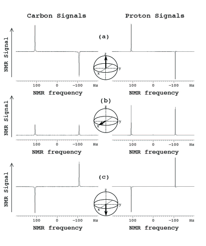
Figure 4: Experimental NMR spectra of carbon and proton for different initial conditions. $\phi=0$ and (a) $\theta=0$, (b) $\theta=\pi/2$ and (c) $\theta=\pi$. The y-axis denotes the signal amplitude in arbitrary units.

Figure 4 shows the experimentally observed NMR signals after Fourier transformation of the corresponding FIDs for the proton and carbon spins for the following initial states: (a) $\theta=0$ (i.e. $\hat{\rho}=\frac{1}{2}\mathbf{1}+\hat{S_{z}}$), (b) $\phi=0,\theta=\pi/2$ (i.e., $\hat{\rho}=\frac{1}{2}\mathbf{1}+\hat{S_{x}}$), (c) $\theta=\pi$ (i.e., $\hat{\rho}=\frac{1}{2}\mathbf{1}-\hat{S_{z}}$).

The amplitudes of the different resonance lines correspond directly to population differences:

$$\begin{array}[]{c}S_{NMR}(\textrm{Proton})\sim P_{1\mu}-P_{2\mu}\\ S_{NMR}(\textrm{Carbon})\sim P_{\mu 1}-P_{\mu 2},\end{array}$$ (49)

where $\mu=1$ for the resonance line with positive frequency and $\mu=2$ for the negative frequency line. From these populations, we determine the initial condition by inverting Eq. (12).

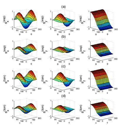
Figure 5: (Color Online) Experimental quantum state tomography for the general initial state $\vec{s}(r,\theta,\phi)$ [see Eq. (46)]. We compare the results from measuring a single observable of the combined system S+A (rows (a) and (b)) with the results from the conventional measurement scheme using three noncommutative measurements of the system S (rows (c) and (d)). In both cases, the expectation values $s_{x},s_{y},s_{z}$, are shown from left to right as functions of the angles $\theta$ and $\phi$: (a) and (c) for a pure state ($r=1$) and (b) and (d) for a partially mixed state with $r=\frac{1}{2}$.

Fig. 5 summarizes these results for a series of similar experiments, where we chose initial conditions $\vec{s}\left(r,\theta,\phi\right)$ varying $\theta$ from 0 to $\pi$ in increments of $\pi/8$, and $\phi$ from 0 to $2\pi$ with an increment of $\pi/12$. In Fig. 5a, we show the measured components $s_{x}^{\left(\exp\right)},s_{y}^{\left(\exp\right)},s_{z}^{\left(\exp\right)}$ for pure states ($r=1$), while (b) shows the corresponding results for mixed states with $r=\frac{1}{2}$. The experiments cover a wide range of points on and within the Bloch sphere. The experimental results clearly show the expected cosine and sine modulations (46), indicating that the measurement network is effective for all these input states. The average fidelity over all $N=9\times 13$ measured states is

$$F_{av}=\frac{1}{N}\sum_{1}^{N}\frac{Tr(\hat{\rho}_{in}\hat{\rho}_{exp})}{\sqrt{Tr(\hat{\rho}_{in}^{2})Tr(\hat{\rho}_{exp}^{2})}}\approx 0.99$$

for both cases, $r=1$ and $r=\frac{1}{2}$.

The experimental data shown in Fig. 5 were obtained with the “short period expansion” technique of section VI A, i.e., the propagator $\hat{U}(\tau)$ was approximately realized by Eq. (37) by repeating the sequence (39) twice. We also repeated the experiment with the “exact decomposition” technique. The propagator $\hat{U}(\tau)$ was realized by the exact decomposition Eq. (40). The corresponding pulse sequence was obtained by combining the sequences (42) with (44). The results that we obtained were similar to those represented in Fig. 5, but the fidelities were slightly lower. This difference is probably due to the larger number of pulses in this experiment.

VII.3 Precision of the Measurement

An alternative measure of the precision of the measurement is the distance $D$ between the experimentally determined state $\vec{s}_{exp}$ and the ”true” input state $\vec{s}$. In terms of the parametrization (46), the trace distance between the two density operators is

$$D(\vec{s}_{exp},\vec{s})=\frac{\left|\vec{s}_{exp}-\vec{s}\right|}{2}=\frac{1}{2}\sqrt{\Delta s_{x}^{2}+\Delta s_{y}^{2}+\Delta s_{z}^{2}}$$ (50)

where $\Delta s_{\nu}=s_{\nu}^{(exp)}-s_{\nu}(\nu=x,y,z)$.

Writing $\Delta P$ for the experimental errors and using the definition (12) of the transfer matrix, we find for the distance

$$D(\vec{s}_{exp},\vec{s})=E|\Delta P|,$$ (51)

where

$$E=\frac{1}{2}\sqrt{E_{x}^{2}+E_{y}^{2}+E_{z}^{2}}$$ (52)

and

$$\begin{array}[]{l}E_{x}=\frac{\Delta s_{x}}{\Delta P}=\frac{1}{det(\tilde{\mathcal{M}})}\sum_{k=1}^{4}A_{k2}\\ E_{y}=\frac{\Delta s_{x}}{\Delta P}=\frac{1}{det(\tilde{\mathcal{M}})}\sum_{k=1}^{4}A_{k3}\\ E_{z}=\frac{\Delta s_{x}}{\Delta P}=\frac{1}{det(\tilde{\mathcal{M}})}\sum_{k=1}^{4}A_{k4}\end{array}.$$ (53)

The $A_{kj}$ are the cofactors of the minors $\tilde{\mathcal{M}}_{kj}$ of the transfer matrix

$$\tilde{\mathcal{M}}=\frac{1}{2}\mathcal{M}\left(\begin{array}[]{cccc}1&0&0&1\\ 0&1&-i&0\\ 0&1&i&0\\ 1&0&0&-1\\ \end{array}\right).$$

The determinant of this matrix is $det(\tilde{\mathcal{M}})=-\frac{1}{4}i\Delta$. Therefore, the error propagation coefficients $E_{\alpha}$ depend only on the mapping $\mathcal{M}$. The smaller they are, the higher the precision of the resulting measurement.

As Eq. (53) shows, the error propagation scales inversely with the determinant $\Delta$ of the transfer matrix $\mathcal{M}$. We illustrate this dependence in Fig. 6a), where we plot the two quantities as a function of the coupling evolution time $\tau$. The minima of $E$ occur near the maxima of $|\Delta|$, and when $|\Delta|=0$, $E$ tends to infinity. In this range, it is impossible to determine the state $\rho$ by such a measurement. A closer look shows that the minima of $E$ do not occur exactly at the maxima of $|\Delta|$. The difference arises from the numerators in (53).

In our experiment, the experimental uncertainties are $\Delta P\approx 5\%$. For the chosen experimental parameters, this results in an average distance $D_{av}(\vec{s}_{exp},\vec{s})=0.04$ for $r=1$ and $0.03$ for $r=\frac{1}{2}$. The distance measurement $D$ and the fidelity measurement F are related by $1-F\leq D\leq\sqrt{1-F^{2}}$ Nielsen and Chuang (2000).

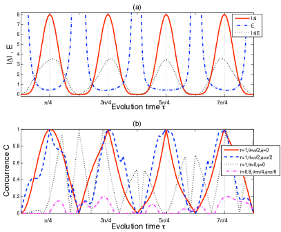
Figure 6: (Color Online) (a) Error coefficient $E$ (solid line), magnitude of the determinant $|\Delta|$ (dashed line) and their product (dotted line) vs. evolution time $\tau$ under the Hamiltonian $\hat{H}^{opt}$ of the example (c) in Sec. IV B. (b) The concurrence $C$ (i.e, entanglement) evolves with the evolution time $\tau$ under the same Hamiltonian for the different initial states $\hat{\rho}=\frac{1}{2}(\mathbf{1}+r\sin\theta\cos\phi\hat{S_{x}}+r\sin\theta\cos\phi\hat{S_{y}}+r\cos\theta\hat{S_{z}})$ with pure states of $r=1,\theta=\pi/2,\phi=0$ (red solid line), $r=1,\theta=\pi/2,\phi=\pi/2$ (blue dashed line), $r=1,\theta=0,\phi=0$ (black dotted line), and a specific mixed state of $r=0.8,\theta=\pi/4,\phi=\pi/6$ (red dash-dotted line)

.

VII.4 Entanglement

The evolution that transfers information from the system to the assistant can entangle the two qubits with each other. In Fig. 6, we quantify the entanglement generated and relate it to the precision of the measurement. Fig. 6 b) shows the concurrence $C$ during the coupling evolution, calculated as

$$C(t)=max\{\chi_{1}-\chi_{2}-\chi_{3}-\chi_{4},0\},$$

where $\chi_{i}(i=1,2,3,4)$ are the square roots of the eigenvalues of

$$16\,\hat{\varrho}_{t}(S_{y}^{1}S_{y}^{2})\hat{\varrho}_{t}^{*}(S_{y}^{1}S_{y}^{2})$$

in decreasing order, and

$$\hat{\varrho}_{t}=\hat{U}(t)(\hat{\rho}\otimes\frac{1}{2}\mathbf{1})\hat{U}^{\dagger}(t)$$

is the instantaneous density operator.

If the initial state is in the $xy$-plane, the entanglement between the system and assistant is maximized at roughly the same time as the information transfer for these measurements is optimized (as quantified by $|\Delta|$). However, for initial conditions oriented along the z-axis, the entanglement generated by the specific Hamiltonian shows a relatively complicated time dependence and little correlation with the precision of the measurement. For evolution times close to $\tau\approx 5\pi/4$, e.g., the entanglement vanishes, while the measurement error is minimized.

The dash-dotted curve in Fig. 6b) shows the entanglement that is generated for a partially mixed input state with a general orientation ($r=0.8,\theta=\pi/4,\phi=\pi/6$). In this case, the concurrence remains below 0.2 and reaches zero even at the times where the measurement precision is optimized. If the amplitude $r$ is reduced further, the entanglement vanishes, $C(\hat{\varrho}_{t})\equiv 0$, but the precision of the measurement is not affected. We conclude that entanglement between system and assistant is not an essential criterion for the success of this measurement scheme.

VIII CONCLUSION

We have experimentally demonstrated how the complete state of a quantum system can be obtained from the results of repeated measurements with a single, factorized observable $\hat{\Omega}$. The procedure, which involves a controlled interaction between the system under test and a second quantum system, was proposed by Allahverdyan et al. Allahverdyan et al. (2004).

In our experiment, we used a Heisenberg-coupling to transfer information from the system to the assistant. Interactions of this type are found in many physical systems: apart from nuclear spins (like in this work), they also occur in quantum dots Loss and DiVincenzo (1998); Imamogu et al. (1999), donor atoms in silicon Kane (1998); Vrijen et al. (2000), quantum Hall systems Mozyrsky et al. (2001) and electrons on helium Dykman and Platzman (2000).

The precision of this type of measurements depends strongly on the details of the interaction between system and assistant, on the type of Hamiltonian as well as on the duration of the interaction. This can be understood by considering the transfer of information from the state of the system to the measurement results from the single observable: If we describe this transfer of information from $n$ elements of the density operator of the input state by a matrix $\mathcal{M}$, the rank of this matrix must be $n$, i.e. its inverse must exist. In practice, it is necessary to choose a transfer matrix that is far from the singular case, to maximize the precision with which the input state can be calculated from the measurement results.

This initial work has demonstrated the basic possibility of implementing such measurements on the simplest possible quantum system (a single spin 1/2). Of course it is possible to extend the scheme to systems of arbitrary size. Work in this direction is currently under way.

ACKNOWLEDGMENTS

We gratefully acknowledge helpful discussions with Dr. Bo Chong, Dr. Jingfu Zhang and financial support from the DFG through Su 192/19-1. Du. J thanks the support of NSFC of China, CAS and the European Commission under Contract No. 007065 (Marie Curie).

References

• Pauli (1933) W. Pauli, in Handbuch der Physik, edited by H. Geiger and K. Scheel (Springer, Berlin, 1933), vol. 24, p. 98.
• Bohr (1935) N. Bohr, Phys. Rev. 48, 696 (1935).
• Helstrom (1976) C. W. Helstrom, Quantum Detection and Estimation Theory (Academic Press, New York, 1976).
• Chefles (2000) A. Chefles, Contemporary Physics 41, 401 (2000).
• Gill and Guta (2003) R. Gill and M. Guta, arXiv.org:quant-ph/0303020 (2003).
• Bechmann-Pasquinucci and Tittel (2000) H. Bechmann-Pasquinucci and W. Tittel, Phys. Rev. A 61, 062308 (2000).
• Bechmann-Pasquinucci and Peres (2000) H. Bechmann-Pasquinucci and A. Peres, Phys. Rev. Lett. 85, 3313 (2000).
• Welsch et al. (1999) D. Welsch, W. Vogel, and T. Opatrný, Progr. Opt. 39, 63 (1999).
• D’Ariano (1997) G. D’Ariano, In: T. HakioImagelu and A.S. Shumovsky, Editors, Quantum Optics and Spectroscopy of Solids, Editors, Kluwer, Amsterdam pp. 175–202 (1997).
• Leonhardt (1997) U. Leonhardt, Measuring the Quantum State of Light (Cambridge University Press, New York, 1997).
• Ivonovic (1981) I. D. Ivonovic, J. Phys. A: Math. Gen. 14, 3241 (1981).
• Wootters and Fields (1989) W. K. Wootters and B. D. Fields, Ann. Phys. 191, 363 (1989).
• Rehacek et al. (2004) J. Rehacek, B.-G. Englert, and D. Kaszlikowski, Phys. Rev. A 70, 052321 (2004).
• D’Ariano (2002) G. M. D’Ariano, Phys. Lett. A 300, 1 (2002).
• Caves et al. (2002) C. M. Caves, C. A. Fuchs, and R. Schack, Journal of Mathematical Physics 43, 4537 (2002), URL http://link.aip.org/link/?JMP/43/4537/1.
• Du et al. (2006) J. Du, M. Sun, X. Peng, and T. Durt, Phys. Rev. A 74, 042341 (2006).
• Allahverdyan et al. (2004) A. E. Allahverdyan, R. Balian, and T. M. Nieuwenhuizen, Phys. Rev. Lett. 92, 120402 (2004).
• Ernst et al. (1994) R. R. Ernst, G. Bodenhausen, and A. Wokaun, Principles of Nuclear Magnetic Resonance in One and Two Dimensions (Oxford University Press, Oxford, 1994).
• Trotter (1959) H. Trotter, Proc. Amer. Math. Soc. 10, 545 (1959).
• Nielsen and Chuang (2000) M. A. Nielsen and I. L. Chuang, Quantum Computation and Quantum Information (Cambridge Univ. Press, Cambridge, 2000).
• Loss and DiVincenzo (1998) D. Loss and D. P. DiVincenzo, Phys. Rev. A 57, 120 (1998).
• Imamogu et al. (1999) A. Imamogu, D. D. Awschalom, G. Burkard, D. P. DiVincenzo, D. Loss, M. Sherwin, and A. Small, Phys. Rev. Lett. 83, 4204 (1999).
• Kane (1998) B. E. Kane, Nature 393, 133 (1998).
• Vrijen et al. (2000) R. Vrijen, E. Yablonovitch, K. Wang, H. W. Jiang, A. Balandin, V. Roychowdhury, T. Mor, and D. DiVincenzo, Phys. Rev. A 62, 012306 (2000).
• Mozyrsky et al. (2001) D. Mozyrsky, V. Privman, and M. L. Glasser, Phys. Rev. Lett. 86, 5112 (2001).
• Dykman and Platzman (2000) M. Dykman and P. Platzman, Fortschritte der Physik 48, 1095 (2000).