Adiabatic Condition and Quantum Geometric Potential

Abstract

In this paper, we present a $U(1)$-invariant expansion theory of the adiabatic process. As its application, we propose and discuss new sufficient adiabatic approximation conditions. In the new conditions, we find a new invariant quantity referred as quantum geometric potential (QGP) contained in all time-dependent processes. Furthermore, we also give detailed discussion and analysis on the properties and effects of QGP.

Since the establishment of the quantum adiabatic theorem Ehrenfest ; Born ; Schwinger ; Kato in 1923, many fundamental results have been obtained, such as Landau-Zener transition phs.z.sowjetunion , the Gell-Mann-Low theorem Gell-Mann , Berry phase Berry and holonomy Simon . Also the adiabatic processes find their applications in the quantum control and quantum computation Oreg ; J.A.Jone ; Farhi ; Zheng . Recently the common-used quantitative adiabatic condition Schiff ; Messiah ; Landau has been found not able to guarantee the validity of the adiabatic approximation Marzlin ; Tong1 . Consequently various new conditions are conjectured and a series of confusions and debates arise. For example, it was argued Wu that the traditional adiabatic condition did not have any problem at all and that the invalidation of the condition did not mean the invalidation of adiabatic theorem Duki . Some new conditions proposed in Ye ; Tong2 but too rigorous to be used conveniently. Although [22] also adopted the adiabatic perturbation expansion but did not give out proper condition because the basis in MacKenzie can not show certain geometric properties in the adiabatic process. Vertesi pointed out the limitation of traditional condition but also did not give out a proper condition. To solve the problem of insufficiency of traditional adiabatic condition in Marzlin ; Tong1 and clarify the subsequent confusions, in this paper, we present two new sufficient conditions in which the properties and effects of a new invariant quantity are detailedly discussed.

Let us consider a quantum system governed by a time dependent Hamiltonian $H(t)$ and the initial state of the system is an eigenstate $|m,0\rangle$ of $H(0)$ with eigenvalue $E_{m}(0)$, where $m$ denotes the initial value of dimensionless quantum number set. By introducing a dimensionless time parameter $\tau=E_{m}\left(0\right)t/\hbar$ and a dimensionless Hamiltonian $h(\tau)=H(\tau)/E_{m}\left(0\right)$, the time dependent Schrödinger equation reads

$$i\frac{\partial|\Phi_{m}(\tau)\rangle}{\partial\tau}=h(\tau)|\Phi_{m}(\tau)\rangle,\quad\left|\Phi_{m}(0)\right\rangle=\left|{m,0}\right\rangle.$$ (1)

The exact solution $\left|{\Phi_{m}\left(\tau\right)}\right\rangle$ to Eq.(1) is referred to as the system’s $dynamic$ $evolution$ $orbit$ in the Hilbert space.

Furthermore, by considering $\tau$ as a fixed parameter, we can always solve the following quasi-stationary equation

$$h\left(\tau\right)\left|{\varphi_{n}\left(\tau\right)}\right\rangle=e_{n}\left(\tau\right)\left|{\varphi_{n}\left(\tau\right)}\right\rangle.$$ (2)

And the eigenstate $|\varphi_{n}(\tau)\rangle$ with the corresponding initial state $\left|{n,0}\right\rangle$ is referred to as the $adiabatic$ $orbit$ of the system.

For convenience, we denote $\gamma_{nm}\equiv i\left\langle{{\varphi_{n}(\tau)}}\mathrel{\left|{\vphantom{{\varphi_{n}(\tau)}{\dot{\varphi}_{m}(\tau)}}}\right.\kern-1.2pt}{{\dot{\varphi}_{m}(\tau)}}\right\rangle$ and the dot here and below expresses the derivative with respect to time. Apparently, an adiabatic orbit multiplied by an arbitrary time-dependent phase factor still describes the same adiabatic orbit. It is not difficult to see that the following adiabatic orbit

$$\left|{\Phi_{m}^{adia}(\tau)}\right\rangle=\exp\left\{-i\int_{0}^{\tau}[e_{m}(\lambda)-\gamma_{mm}(\lambda)]d\lambda\right\}|{\varphi_{m}(\tau)}\rangle$$ (3)

is invariant under the following $U(1)$ transformation

$$\left|{\varphi_{m}(\tau)}\right\rangle\to e^{if_{m}(\tau)}\left|{\varphi_{m}(\tau)}\right\rangle\;\;(f_{m}(0)=0).$$ (4)

Here $f_{m}(0)=0$ is because of given initial state. We call this adiabatic orbit with special choice of the time-dependent phase factor as the $U(1)$-$invariant$ $adiabatic$ $orbit$.

It is clear that, although the initial conditions $\left|{m,0}\right\rangle$ are the same, the dynamic evolution orbit $|\Phi_{m}(\tau)\rangle$ do not always coincide with the adiabatic orbit $|\varphi_{m}(\tau)\rangle$, or they are not even close to each other. Obviously they coincide if and only if

$$\gamma_{nm}=0\;\;(\forall n\neq m).$$ (5)

Generally speaking, the dynamic evolution orbit $\left|{\Phi_{m}\left(\tau\right)}\right\rangle$ starting from the initial state $\left|{m,0}\right\rangle$ will change among some adiabatic orbits which will cause transitions between different orbits. Our task is to find the proper condition under which the dynamic orbit is sufficiently close to the adiabatic orbit when the Eq.(5) is not satisfied. Since the Hamiltonian $h(\tau)$ is Hermitian, all the $U(1)$-$invariant$ $adiabatic$ $orbits$ in Eq.(3) at a given time constitute a complete orthonormal basis of the system. In this basis, the dynamic evolution orbit of the system reads

$$\left|{\Phi_{m}\left(\tau\right)}\right\rangle=\sum\limits_{n}{c_{n}(\tau)\left|{\Phi_{n}^{adia}\left(\tau\right)}\right\rangle\;,\;\;\;\;}{\left|{\Phi_{m}\left(0\right)}\right\rangle}=\left|{m,0}\right\rangle.$$ (6)

The expansion in Eq.(6) is referred to as the $U(1)$-$invariant$ $adiabatic$ $expansion$ with the time-dependent coefficients. Therefore, the set of coefficients equations reads

$$\dot{c}_{m}(\tau)=i\sum\limits_{n\neq m}{c_{n}(\tau)M(\tau)_{mn}}\;,$$ (7)

where the diagonal elements of the matrix $M(\tau)$ are zero and the non-diagonal elements of $M(\tau)$ read

$$M(\tau)_{mn}=i\left\langle{{\Phi_{m}^{adi}(\tau)}}\mathrel{\left|{\vphantom{{\Phi_{m}^{adi}(\tau)}{\dot{\Phi}_{n}^{adi}(\tau)}}}\right.\kern-1.2pt}{{\dot{\Phi}_{n}^{adi}(\tau)}}\right\rangle\equiv\left|{\gamma_{mn}(\tau)}\right|e^{i\theta_{mn}(\tau)},$$ (8)

where

$$\theta_{mn}(\tau)=\int_{0}^{\tau}{d\lambda\left({e_{m}(\lambda)-e_{n}(\lambda)+\gamma_{nn}-\gamma_{mm}}\right)}+\arg\gamma_{mn}(\tau).$$ (9)

From Eq.(7), it is not hard to get

$$\mathord{\buildrel{\lower 3.0pt\hbox{$\scriptscriptstyle\rightharpoonup$}}\over{C}}(\tau)^{(n+1)}=A(\tau)\mathord{\buildrel{\lower 3.0pt\hbox{$\scriptscriptstyle\rightharpoonup$}}\over{C}}(\tau)$$ (10)

where

$$\begin{array}[]{l}A(\tau)=\sum\limits_{\sum\limits_{h=1}^{k}{\left({j_{h}+1}\right)}=n+1}{\frac{{n!i^{k}}}{{\prod\limits_{p=1}^{k}{j_{p}!}\prod\limits_{l=1}^{k-1}{\left({n+1-\sum\limits_{m=1}^{l}{(j_{m}+1)}}\right)}}}}\\ \;\;\;\;\;\;\;\;\;\;\;\;\;\;\;\;\;\;\;\;\;\;\cdot M^{(j_{1})}M^{(j_{2})}\cdots M^{(j_{k})}\\ \end{array}$$ (11)

and $(n+1)$ denotes the $(n+1)^{th}$ derivation of $\vec{C}(\tau)$ with respect to time. Then we have following theorem

Theorem For an $N$-level quantum system and an arbitrary real $\varepsilon$ and a time period $T$, if the following conditions hold

$$\mathop{\max}\limits_{\forall n,i,j}A(0)_{ij}\;and\;\mathop{\max}\limits_{\forall n,i,j}A(T)_{ij}<B<\infty\;\;\;\;\;\;\;\;\;\;\;\;\;\;\;\;$$ (12)

$$\begin{array}[]{l}\left|{\gamma_{mn}(\tau)}\right|e^{i\dot{\theta}_{mn}}\;can\;be\;expanded\;as\;\sum\limits_{k=1}^{p}{a_{mn}^{k}e^{i\omega_{mn}^{k}\tau}}\\ with\;\mathop{\max}\limits_{\forall n\neq m,k}\left|{a_{mn}^{k}}\right|=D<\infty\\ \end{array}$$ (15)

$$\mathop{\max}\limits_{k}\left|{\frac{1}{{\omega_{mn}^{k}}}}\right|\leq\frac{\varepsilon}{{2pN(N-1)BD}}\equiv\varepsilon^{\prime}<1\;with\;\varepsilon+\varepsilon^{\prime}\leq 1.$$ (16)

then the probability of finding dynamical orbit in the adiabatic orbit $\left|{\Phi_{m}^{adi}(\tau)}\right\rangle$ is greater than $\left({1-\delta}\right)^{2}\;with\;\delta=\varepsilon/(1-\varepsilon^{\prime})$.

$Proof$: From Eq.(7) and the conditions above, we have

$$\begin{array}[]{l}\left|{c_{m}(T)-1}\right|=\left|{\sum\limits_{n\neq m}{\int_{0}^{\infty}{d\tau\left({c_{n}(\tau)\sum\limits_{k=1}^{p}{a_{mn}^{k}e^{i\omega_{mn}^{k}\tau}}}\right)}}}\right|\\ =\left|{\sum\limits_{n\neq m}{\sum\limits_{k=1}^{p}{a_{mn}^{k}}\sum\limits_{q=0}^{\infty}{(-1)^{q}\frac{{c_{n}(T)^{(q)}e^{i\omega_{mn}^{k}T}-c_{n}(0)^{(q)}}}{{\left({i\omega_{mn}^{k}}\right)^{q+1}}}}}}\right|\\ \leq\sum\limits_{n\neq m}{\sum\limits_{k=1}^{p}{\sum\limits_{q=0}^{\infty}{\left|{2NBD\left({\frac{\varepsilon}{{2pBDN(N-1)}}}\right)^{q+1}}\right|}}}=\frac{\varepsilon}{{1-\varepsilon^{\prime}}}\\ \end{array}$$ (17)

Namely,

$$1-\left|{c_{m}(T)}\right|\leq\left|{1-c_{m}(T)}\right|\leq\frac{\varepsilon}{{1-\varepsilon^{\prime}}}.$$ (18)

Therefore, the probability of finding dynamical orbit in the adiabatic orbit $\left|{\Phi_{m}^{adi}(\tau)}\right\rangle$ is

$$P_{m}(T)=\left|{c_{m}(T)}\right|^{2}\geq\left({1-\frac{\varepsilon}{{1-\varepsilon^{\prime}}}}\right)^{2}.$$ (19)

Thus we prove the theorem.

Although Eq.(12-14) in the $theorem$ are sufficient, however, it is somewhat too complicated. It is not hard to find for any $N$-level Hamiltonian with both time-independent terms of $|\gamma_{nm}|$ and $\dot{\theta}_{nm}$ satisfying Rydberg-Ritz Combination Principle(RRCP) $\dot{\theta}_{nl}+\dot{\theta}_{lm}=\dot{\theta}_{nm}$, for an arbitrary real $0\leq\delta\ll 1$, when the following condition holds

$$\max_{\forall m\;and\;k,n\neq m}\frac{{\left|{\gamma_{km}}\right|}}{{\left|{\dot{\theta}_{nm}}\right|}}\leq\frac{\delta}{{\sqrt{N-1}}}$$ (20)

viz.,

$$\max_{\forall m\;and\;k,n\neq m}\frac{{\left|{\gamma_{km}}\right|}}{{\left|{e_{n}(\tau)-e_{m}(\tau)+\Delta_{mn}(\tau)}\right|}}\leq\frac{\delta}{{\sqrt{N-1}}}$$ (21)

where

$$\Delta_{mn}\left(\tau\right)\equiv{\gamma_{mm}\left(\tau\right)-\gamma_{nn}\left(\tau\right)+\frac{d}{{d\tau}}\arg\gamma_{nm}\left(\tau\right)}\;\;(\forall n\neq m).$$ (22)

then the probability of finding dynamical orbit in the adiabatic orbit $\left|{\Phi_{m}^{adi}(\tau)}\right\rangle$ is greater than $(1-\delta)^{2}$.

Proof:   Denote $c^{\prime}_{m}(\tau)=e^{i\omega_{m}\tau}c_{m}(\tau)$ with $\omega_{m}-\omega_{n}=\dot{\theta}_{mn}$. Then, $c^{\prime}_{m}(\tau)$ satisfy equations

$$i\frac{\partial}{\partial\tau}\vec{C^{\prime}}(\tau)=\Pi\vec{C^{\prime}}(\tau)$$ (23)

where $\vec{C^{\prime}}(\tau)=(c^{\prime}_{1}(\tau),c^{\prime}_{2}(\tau),\ldots,c^{\prime}_{N}(\tau))^{T}$, $\Pi$ is a self-adjoint matrix, $\Pi_{kk}=\omega_{k}$ and $\Pi_{kl}=|\gamma_{kl}|$. Denote eigenvalues of $\Pi$ as $\eta_{m}$, we have Proof

$$|\eta_{m}-\omega_{m}|\leq\sqrt{\sum\limits_{k\neq m}2|\gamma_{km}|^{2}}.$$ (24)

If unitary matrix $U$ diagonalizes $\Pi$, then $U\Pi U^{{\dagger}}=diag\left\{{\eta_{1},\eta_{2},\cdots,\eta_{N}}\right\}$, that is $U_{ik}\Pi_{kj}=\eta_{i}U_{ij}$, thus $U_{ij}=\sum\limits_{k\neq j}\frac{|\gamma_{kj}|}{\eta_{i}-\omega_{j}}U_{ik}$. When condition (21) holds, then

$$\frac{{\left|{\gamma_{kj}}\right|}}{{\eta_{i}-\omega_{j}}}\leq\frac{\delta}{{\sqrt{N-1}}}+\sqrt{\frac{2}{{N-1}}}o(\delta^{2}),\forall i\neq j$$ (25)

so $|U_{ij}|\leq\left({\delta+\sqrt{2}o(\delta^{2})}\right)/\sqrt{N-1}$ and $|U_{ii}|\geq 1-\delta/2-o(\delta^{2})$.

$\vec{C^{\prime}}(\tau)$ can be solved exactly as $\Pi$ is time-independent

$$\vec{C^{\prime}}(\tau)=e^{i\Pi\tau}\vec{C^{\prime}}(0).$$ (26)

Applying initial condition $c^{\prime}_{k}(0)=\delta_{km}$, the exact solution of $c^{\prime}_{m}(\tau)$ is $\sum\limits_{k}|U_{mk}|^{2}e^{i\eta_{k}t}$. Thus, $|c_{m}(\tau)|\geq 1-\delta$, then the probability of finding dynamical orbit in the adiabatic orbit $\left|{\Phi_{m}^{adi}(\tau)}\right\rangle$ is $P_{m}(\tau)\geq(1-\delta)^{2}$. Thus the proof is completed.

The premises of Eq.(21) on Hamiltonian are non-trivial. For any general 2D system $h(\tau)=e_{+}(\tau)|+,\tau\rangle\langle+,\tau|+e_{-}(\tau)|-,\tau\rangle\langle-,\tau|$, after applying a transformation $\tau\rightarrow\tau^{\prime}=g^{-1}(\tau)$ with $g(\tau)\propto\int_{0}^{\tau}{|\left\langle{+,\lambda}\right|\frac{d}{{d\lambda}}\left|{-,\lambda}\right\rangle|d\lambda}$, then we can forcibly get $e^{\prime}_{-}-e^{\prime}_{+}+\Delta^{\prime}_{+-}=constant$ which makes the final time-dependent 2D system satisfying the limitations of Eq.(21).

In condition Eq.(21), there appears a new interesting quantity $\Delta_{mn}$ referred to as $quantum$ $geometric$ $potential$ (QGP) for following three reasons. First, QGP is also $U(1)$-invariant under the transformation Eq.(4). Second, the integral of QGP over a closed smooth curve is the difference of Berry phases of different adiabatic orbits. And the last reason is that the value of QGP depends only on the path and measure of adiabatic orbit or, in other words, $\Delta_{mn}(\tau)/\left|{\gamma_{mn}}\right|\;(\forall n\neq m)$ is invariant under any transformation $\tau\rightarrow\tau^{\prime}=f(\tau)$. Furthermore, It can be proved that in 2D systems $\Delta_{mn}(\tau)/2\left|{\gamma_{mn}}\right|$ is just the geodesic curvature of spherical curve corresponding to the adiabatic orbit on the surface of Bloch sphere or 2D real Ray space.

Proof: Generally, we can write the Hamiltonian of a 2D system as $h\left(\tau\right)=A\left(\tau\right)+B\left(\tau\right)\vec{n}\left(\tau\right)\cdot\vec{\sigma},$ where $\vec{n}\left(\tau\right)=\left({\sin\theta\left(\tau\right)\cos\varphi\left(\tau\right),\sin\theta\left(\tau\right)\sin\varphi\left(\tau\right),\cos\theta\left(\tau\right)}\right)$. Choosing appropriate phases, the Hamiltonian’s instantaneous eigenstates or adiabatic orbits read

$$\left\{\begin{array}[]{l}\left|{+,\tau}\right\rangle=\cos\frac{{\theta\left(\tau\right)}}{2}\left|0\right\rangle+e^{i\varphi\left(\tau\right)}\sin\frac{{\theta\left(\tau\right)}}{2}\left|1\right\rangle\\ \left|{-,\tau}\right\rangle=\sin\frac{{\theta\left(\tau\right)}}{2}\left|0\right\rangle-e^{i\varphi\left(\tau\right)}\cos\frac{{\theta\left(\tau\right)}}{2}\left|1\right\rangle\\ \end{array}\right..$$ (29)

It’s quite clear that polarization vectors of the above two adiabatic orbits point to $\vec{n}\left(\tau\right)$ and $-\vec{n}\left(\tau\right)$ at time $\tau$, respectively. Considering the adiabatic orbit $|+,\tau\rangle$, the QGP of this orbit can be easily calculated as

$$\Delta_{mn}=\frac{{\dot{\theta}\ddot{\phi}\sin\theta+2\dot{\theta}^{2}\dot{\phi}\cos\theta+\dot{\phi}^{3}\sin^{2}\theta\cos\theta-\dot{\phi}\ddot{\theta}\sin\theta}}{{\dot{\theta}^{2}+\left({\dot{\phi}\sin\theta}\right)^{2}}}.$$ (30)

As a comparison, we will calculate the geodesic curvature of the spherical curve $\vec{r}\left(\tau\right)=\vec{n}\left(\tau\right)$.

$$\rho = \left(\vec{r}\times\frac{d\vec{r}}{ds}\right)\cdot\frac{d^{2}\vec{r}}{ds^{2}}$$ (31)

$$= \frac{{\dot{\theta}\ddot{\phi}\sin\theta+2\dot{\theta}^{2}\dot{\phi}\cos\theta+\dot{\phi}^{3}\sin^{2}\theta\cos\theta-\dot{\phi}\ddot{\theta}\sin\theta}}{{\left({\sqrt{\dot{\theta}^{2}+\left({\dot{\phi}\sin\theta}\right)^{2}}}\right)^{3}}},$$

where curve element

$$ds=\left|d\vec{r}\right|=\sqrt{\dot{\theta}+\left({\dot{\phi}\sin\theta}\right)^{2}}d\tau=2|\gamma_{mn}|d\tau.$$

Then we get

$$\frac{\Delta_{mn}}{2|\gamma_{mn}|}=\rho.$$ (32)

In the following part, two models will be presented to show Eq.(21) is a good sufficient adiabatic condition and the effect of QGP is significant. Firstly, we shall study a spin-half particle in a magnetic field. The Hamiltonian of the system is

$$h(\tau)=\eta\sigma_{z}+\xi\left[{\sigma_{x}\cos\left({2K\eta\tau}\right)+\sigma_{y}\sin\left({2K\eta\tau}\right)}\right],$$ (33)

where $\eta=\hbar\omega_{0}/E_{\pm},\;\xi=\hbar\omega/E_{\pm}\;{\rm{and}}\;E_{\pm}=\sqrt{\eta^{2}+\xi^{2}}\;{\rm{are}}\;{\rm{all}}\;{\rm{constants}}$. Obviously, Eq.(21) is a sufficient adiabatic condition for this kind of Hamiltonian. Properly choosing phases, two adiabatic orbits can be written as

$$\left\{\begin{array}[]{l}\left|{\varphi_{+}(\tau)}\right\rangle=\cos\left({\frac{\theta}{2}}\right)\left|0\right\rangle+e^{2iK\eta\tau}\sin\left({\frac{\theta}{2}}\right)\left|1\right\rangle\\ \left|{\varphi_{-}(\tau)}\right\rangle=\sin\left({\frac{\theta}{2}}\right)\left|0\right\rangle-e^{2iK\eta\tau}\cos\left({\frac{\theta}{2}}\right)\left|1\right\rangle\\ \end{array}\right.,$$ (36)

where $\cos\theta=\eta/\sqrt{\eta^{2}+\xi^{2}}$. Consider the adiabatic orbit $|\varphi_{+}(\tau)\rangle$, we have QGP, $\Delta_{+-}=2K\eta\cos\theta$. It is easy to obtain the expression of the new adiabatic condition of Eq.(21)

$$\left|{\sqrt{\eta^{2}+\xi^{2}}-K\eta\cos\theta}\right|\gg\left|{K\eta\sin\theta}\right|.$$ (37)

Suppose the initial state of the system is $|+,0\rangle$, we have the fidelity between the dynamic evolution orbit and the adiabatic orbits at time $\tau$

$$\begin{array}[]{l}F(\tau)=\sqrt{\cos^{2}(A\tau)+\sin^{2}(A\tau)\left[{\frac{{(1-K)\eta\cos\theta+\xi\sin\theta}}{A}}\right]^{2}}\\ \end{array}$$ (39)

where $A=\sqrt{\left({1-K}\right)^{2}\eta^{2}+\xi^{2}}$ is also a constant parameter.

If we choose $\eta\gg\xi$ and $K\simeq 1$, then the traditional condition [16] is satisfied but the new condition Eq.(21) is not. Meanwhile, the fidelity $F\left(\tau\right)\approx\sqrt{1-\cos^{2}\theta\sin^{2}\left({A\tau}\right)}\nrightarrow 1$ when $\tau$ is not too small. Thus, even though the traditional condition is satisfied and we might regard the system as slowly changing one, the quantum adiabatic approximation may be unfaithful description of the system because of the effect of the QGP.

While if we choose $\eta\gg\xi$ with $K\gg 1$ and $K\gg\eta$, in this case, the QGP is much larger than the difference of the instantaneous energy eigenvalues, and the new condition Eq.(21) is satisfied while the traditional one is not. Now we have $F\left(\tau\right)\approx\sqrt{1-\sin^{2}\theta\sin^{2}\left({A\tau}\right)}\approx 1$. Therefore, the QGP can help to guarantee the validity of the adiabatic approximation despite the difference of energy eigenvalues is too small to satisfy the traditional condition.

Next, notifying that if QGP has same sign as the corresponding difference of energy eigenvalue, it will positively guarantee the system evolution to be adiabatic. Moreover, if $\left|{\Delta_{nm}}\right|/\left|{\left\langle{n}\mathrel{\left|{\vphantom{n{\dot{m}}}}\right.\kern-1.2pt}{{\dot{m}}}\right\rangle}\right|\gg 1$, with Eq.(21), then the evolution may be adiabatic whether the adiabatic orbit moves slowly or fast. Thus we shall present an interesting Hamiltonian for illustrating QGP may be helpful to construct robust system. Consider a 2D system governed by Hamiltonian $h(\tau)=\eta\sigma_{z}+e^{-i\eta\sigma_{z}\tau}(\eta_{0}\sigma_{x}+\eta_{1}e^{i\eta_{2}\sigma_{x}\tau}\sigma_{z}e^{-i\eta_{2}\sigma_{x}\tau})e^{i\eta\sigma_{z}\tau}$ with $\eta_{0}/\eta\gg 1\ \text{and }\eta_{0}/\eta_{1}\gg 1$. The density matrixes of adiabatic orbits read

$$\rho^{adi}_{\pm}(\tau)=\frac{1}{2}\pm\frac{\eta\sigma_{z}+e^{-i\eta\sigma_{z}\tau}(\eta_{0}\sigma_{x}+\eta_{1}e^{i\eta_{2}\sigma_{x}\tau}\sigma_{z}e^{-i\eta_{2}\sigma_{x}\tau})e^{i\eta\sigma_{z}\tau}}{2N(\tau)},$$ (40)

where $N(\tau)=\sqrt{\eta_{0}^{2}+(\eta+\eta_{1}\cos 2\eta_{2}\tau)^{2}+\eta_{1}^{2}\sin^{2}2\eta_{2}\tau}$. The density matrixes of the evolution orbits starting from the corresponding initial states of adiabatic orbits reads

$$\rho_{\pm}(\tau)=\frac{1}{2}U(\tau)\left(1\pm\frac{\eta_{0}\sigma_{x}+(\eta_{1}+\eta)\sigma_{z}}{N(0)}\right)U^{{\dagger}}(\tau),$$ (41)

where $U(\tau)=e^{-i\eta\sigma_{z}\tau}e^{i\eta_{2}\sigma_{x}\tau}e^{-i((\eta_{0}+\eta_{2})\sigma_{x}+\eta_{1}\sigma_{z})\tau}$ and the initial states are $\rho^{adi}_{\pm}(0)$. The probabilities of staying in the corresponding adiabatic orbits are

$$P_{\pm}(\tau) = \frac{1}{2N(0)N(\tau)}\left(\eta_{0}^{2}+\eta_{1}^{2}+\eta^{2}\cos 2\eta_{2}\tau+2\eta\eta_{1}\cos^{2}\eta_{2}\tau\right.$$ (42)

$$+\frac{2\tilde{\eta}^{4}}{\bar{\eta}^{2}}\sin^{2}\bar{\eta}\tau-\frac{4\eta(\eta_{0}+\eta_{2})\tilde{\eta}^{2}}{\bar{\eta}^{2}}\cos^{2}\eta_{2}\tau\sin^{2}\bar{\eta}\tau$$

$$+\left.\frac{\eta\tilde{\eta}^{2}}{\bar{\eta}}\sin 2\bar{\eta}\tau\sin 2\eta_{2}\tau\right)+\frac{1}{2}.$$

Here $\bar{\eta}=\sqrt{\eta^{2}_{1}+(\eta_{0}+\eta_{2})^{2}}\ \text{and}\ \tilde{\eta}=\sqrt{\eta\eta_{0}+\eta\eta_{2}+\eta_{2}\eta_{1}}$. Since $\eta_{0}/\eta\gg 1\ \text{and }\eta_{0}/\eta_{1}\gg 1$, then probabilities will obtain a lower bound $P_{\min}$ independent on the magnitude of $\eta_{2}$: $P_{\min}=1-\left({\eta+\eta_{1}}\right)^{2}/N(0)^{2},$ which approach to 1. It’s not hard to verify when $\eta_{2}>>\eta$, $\Delta_{+-}$ has the same sign as $E_{-}-E_{+}$, and $\left|{\Delta_{+-}}\right|/\left|{\left\langle{+}\mathrel{\left|{\vphantom{+{\dot{-}}}}\right.\kern-1.2pt}{{\dot{-}}}\right\rangle}\right|\simeq\eta_{0}/\eta_{1}\gg 1$. When $\eta_{2}$ is large, the velocity of the adiabatic orbit has the same order of magnitude of $\eta_{2}$, at this time, the adiabatic orbit fast oscillates around the exact dynamic evolution orbit, but the evolution of the system still keeps adiabatic. Fig.1 shows evolution orbit and adiabatic orbit for $\eta_{0}/\eta=\eta_{0}/\eta_{1}=20\;{\rm{and}}\;\eta_{0}/\eta_{2}=0.2$.

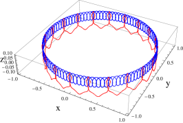
Figure 1: evolution orbit(red line) and adiabatic orbit(blue line).

This kind of models allows the parameters of the system have a certain variant range, as long as the adiabatic condition Eq.(21) holds. Thus we may conclude that the QGP may help setting up robust systems which may tolerate faults of the system itself. Another interesting hint from this model is that the adiabatic orbit may be very complicated comparing with evolution orbit, which is counterintuitive from the traditional opinion.

For a short summary, it is worthwhile to point that, by the $theorem$ or new adiabatic condition Eq.(21), the problems showed in [13,14] has not existed because the relation between systems $a$ and $b$ constructed in [13,14] does not guarantee them. Apparently, different from those conditions in Tong2 ; MacKenzie ; Vertesi , our conditions are presented in a more natural way full of geometric interpretation. One more hint we may get here is that we should more carefully deal with the phase appearing in the time-dependent evolution. It is just improperly handling the phase of Eq.(8) in the work of predecessors Schiff ; Messiah that led to their improper traditional condition and later contradiction in Marzlin ; Tong1 . The condition (21) also implies a modification of the difference of energy eigenvalues is necessary. Description of the time-dependent evolution might be more precise and more appropriate via replacing $e_{m}\left(\tau\right)-e_{n}\left(\tau\right)$ by $e_{m}\left(\tau\right)-e_{n}\left(\tau\right)+\Delta_{mn}$. And a related experiment Du for verifying the effect of QGP has been finished. The experiment also found the characteristic frequency of a kind of time-dependent systems should be corrected via QGP. The experiment also illustrated the QGP should reflect some properties of time-dependent systems, and is not just a convenient mathematical technique. As it is shown in our paper, QGP may play an important role in some kinds of time-dependent procedure, but what role it may play in general time-dependent system is not clear now. We guess non-trivial QGP will more or less affect the evolution procedure of time-dependent system.

In conclusion, according to the concepts of $U(1)$-invariant adiabatic orbit and $U(1)$ invariant expansion stated in this paper, we present a theorem and a new sufficient adiabatic condition, from which we get an interesting quantity QGP with its effects and geometric properties detailedly discussed. At the end we present two models to show the significant effect of QGP on the evolution.

References

(1)
P. Ehrenfest, Ann. Phys. (Berlin) 356, 327 (1916).
(2)
M. Born and V. Fock, Z. Phys. 51, 165 (1928).
(3)
J. Schwinger, Phys. Rev. 51, 648 (1937).
(4)
T. Kato, J. Phys. Soc. Jpn. 5, 435 (1950).
(5)
L. D. Landau, Zeitschrift 2, 46 (1932); C. Zener, Proc. R. Soc.
London A 137, 696 (1932).
(6)
M. Gell-Mann and F. Low, Phys. Rev. 84, 350(1951).
(7)
M. V. Berry, Proc. R. Soc. A 392, 45 (1984).
(8)
B. Simon, Phys. Rev. Lett. 51, 2167(1983).
(9)
J. Oreg , Phys. Rev. A 29, 690 (1984); S. Schiemann
, Phys. Rev. Lett 71, 3637 (1993); P. Pillet, , Phys.
Rev. A 48, 845 (1993).
(10)
J. A. Jone et al., Nature(London)403,869(2000).
(11)
E. Farhi , quant-ph/0001106; A. M. Childs ,
Phys. Rev. A 65, 012322 (2002).
(12)
S. B. Zheng, Phys. Rev. Lett, 95, 080502(2005).
(13)
K. P. Marzlin and B. C. Sanders, Phys. Rev. Lett. 93, 160408(2004).
(14)
D. M. Tong , Phys. Rev. Lett. 95, 110407(2005).
(15)
L. I. Schiff, Quantum Mechanics, 3rd.ed. McGraw Hill N.Y.1968;
D. Bohm, Quantum Theory(Prentic-Hall Inc. N.Y. 1951).
(16)
A. Messiah, Quantum Mechanics, North-Holland, Amsterdam 1962.
(17)
L. D. Landau, E. M. Lifshitz, Quantum Mechanics, 3rd. ed.
Pergamon, Oxford.
(18)
Z. Wu , quant-ph/0411212.
(19)
S. Duki , Phys. Rev. Lett. 97, 128901 (2006);
quant-ph/0510131.
(20)
M. Y. Ye , quant-ph/0509083; D. Comparat,
quant-ph/0607118.
(21)
D. M. Tong et al., Phys. Rev. Lett. 98, 150402(2007).
(22)
R. MacKenzie , Phys. Rev. A 73, 042104 (2006).
(23)
T. Vertesi and R. Englman, Phys. Lett. A 353, 11 (2006).
(24)
Jiangfeng Du, Lingzhi Hu, Ya Wang, Jianda Wu, Meisheng Zhao, Dieter
Suter, Is the quantum adiabatic theorem consistent?
, quant-ph/arXiv:0801.0361
(25)
Denote , where
.
Denote ’s eigenvalues as . One can immediately see
. Applying the Wielandt-Hoffman theorem on
eigenvalues of self-adjoint matrixes, one
have This is just Eq.(24).