Entropy Moments Characterization of Statistical Distributions

Abstract

This letter reports two moment extensions of the entropy of a distribution. By understanding the traditional entropy as the average of the original distribution up to a random variable transformation, the traditional moments equation become immediately applicable to entropy. We also suggest an alternative family of entropy moments. The discriminative potential of such entropy moment extensions is illustrated with respect to different types of distributions with otherwise undistinguishable traditional entropies.

‘Looking into each globe, you see a blue city, the model of a different Fedora.’ (I. Calvino, Invisible Cities)

Given a statistical distribution $p(x)$, where $x$ is the respective random variable, an important problem is to try to synthetize its most important features into as few measurements $f_{i}$, $i=1,2,\ldots,N$ as possible. Although a distribution incorporates all information about the respective random variable $x$, it typically involves a large number of values. While continuous distributions have infinite values, discrete distributions typically involve a large number of bins. However, the summarization of a distribution in terms of a few respective functionals is not straightforward and ultimately depends on specific goals. For instance, one may be interested in intervals of regularity along the distributions, or in the overall dispersion. Generally, it is useful to remove the redundancy from the distributions, leaving out only the most informative variations and singularities. Traditional functionals of distributions include the respective moments given as

$$M(p(x),k)=\int_{I}x^{k}p(x)dx$$ (1)

where $I$ is the domain of $p(x)$, i.e. its sampling space. Observe that these moments have the same dimensionality as the original random variable $x$. The first moment corresponds to the average and the second moment is related to the variance of the random variable $x$. It is know from statistical theory (e.g. Shohat and Tamarkin (1943); Dudewicz and Mishra (1988)) that the set of all infinite moments can, under certain conditions (the so-called moment problem), provide a complete mapping of the original distribution, in the sense that the latter can be recovered from the former. Generally, increasing information about the features of the original distribution can be obtained by considering a larger number of moments. Another important functional of a statistical distribution is its respective entropy (e.g. Greven et al. (2003); Sethna (2006); Cover and Thomas (1991)), which is defined as

$$e(p(x))=-\int_{I}p(x)log(p(x))dx$$ (2)

This measurement becomes zero for distributions involving identical values of $x$, being maximized for uniform distributions, i.e. identical values of $p(x)$ along $I$. The entropy measurement exhibits several particularly relevant properties, including its intrinsic relationship with statistical physics (e.g. Landau and Lifshitz (1980)), entropy maximization (e.g. Boyd and Vandenberghe (2005); Cover and Thomas (1991)), information theory and channel capacity (e.g. Cover and Thomas (1991)). The entropy is also invariant to transformation of the values of $x$, i.e. the entropy of the distribution of $x$ is identical to the distribution of the new random variable $y=f(x)$, where $f$ is any one-to-one function. Yet, typically the entropy is considered as an isolated measurement.

In this article we suggest a family of entropy-based measurements which provide enhanced information about the original distribution. First, we show that the entropy can be understood as a special case of the first moment, where the values of the random variable $x$ are substituted by the adimensional quantity $log(p(x))$, i.e. the weights in the average definition are exchangec by the logarithm of the distribution values. By doing so, it becomes possible to calculate all respective moments and central moments, which are henceforth called the entropy moments and entropy central moments. We illustrate the power of such additional statistical measurements with respect to the discrimination between important types of statistical distributions.

We henceforth focus our attention on discrete distributions represented in the continouous space of the variable $x$, i.e.

$$p(x)=p(x_{i})=\sum_{i=1}^{N}p(i)\delta(x_{i})$$ (3)

where $x$ is a continuous variable in $I=[a,b]$ and $\delta(x_{i})$ is the Dirac’s delta function placed at $x_{i}$, i.e. $\delta_{(}x_{i})=\delta_{x-x_{i}}$, with $i=1,2,\ldots,N$. Therefore, $p(x_{i})$ can be used to represent any relative frequency histogram. The moments of this distribution are immediately given by Equation 1.

Now, by introducing the new random variable $y_{i}=log(p(x_{i}))$, we can rewrite the entropy as

$$e(p(x_{i}))=-\int_{I}p(x_{i})log(p(x_{i}))dx=-\int_{J}y_{i}p(y_{i})dy$$ (4)

where $J$ is the mapped version of the interval $I$, i.e. $J=[min(log(p(x_{i}))),max(log(p(x_{i})))]$. Observe that $p(x_{i})=p(y_{i})$ for any $i=1,2,\ldots,N$. We have from Equation 4 that the traditional entropy can be understood as the negative of the first moment (i.e. average) of the distribution of the transformed random variable $y_{i}=log(p(x_{i}))$. The extension to higher order moments is straightforward and yields the respective moments given by Equation 5.

$$\mathrm{ME}(p(x_{i}),k)=-\int_{J}(y_{i})^{k}p(y_{i})dy$$ (5)

$$\mathrm{FE}(p(x_{i}),k)=log\left(-\int_{J}(p(y_{i}))^{k}y_{i}dy\right)$$ (6)

We necessarily have that $\mathrm{ME}(p(x_{i}),k)=\mathrm{ME}(p(y_{i}),k)$ and $\mathrm{FE}(p(x_{i}),k)=\mathrm{FE}(p(y_{i}),k)$. Observe that the non-dimensionality of $y_{i}$ is immediately extended to the entropy moments. In addition, the consideration of $y_{i}$ as the weights for the moment calculation implies the respectively induced distribution $p(y_{i})$ to be sorted into ascending order. It should be also observe that the successive entropy moments $ME$ tend to present inverse signals. Because of the moment mapping theorem, we have that all the information in the original distribution $p(x_{i})$ is captured by the infinite set of respective moments. Therefore, these additional entropy-based measurements provide an interesting complementation of the traditional entropy, allowing a more comprehensive characterization of the original distribution in terms of a set of respective functionals, in direct analogy with the role of the traditional moments. The alternative entropy moments defined by Equation 6 have been found to allow particularly discriminating measurements. In this definition, the most external logarithm is used in order to obtain more manageable values.

In the remainder of this article, we provide a series of examples of the potential of the entropy moments and alternative entropy moments. First, we consider distributions of the type $p(x_{i})=w\ exp(ci)$, $x_{i}=(i-1)\Delta$ and $\Delta=(b-a)/(N-1)$,where $c$ is a real value such that $0\leq c$ and $w$ is a normalizing constant ensuring $\int_{I}p(x_{i})dx=1$. Observe that this distribution becomes the uniform distribution when $c=0$ and the constant distribution when $c\rightarrow\infty$. Figure 1 illustrates the distribution $p(x_{i})=w\ exp(ci)$ (a-d) and the normal distribution $q(x_{i})=s\ exp(-0.5((ci-\mu)/\sigma)^{2})$ (i-l), where $s$ is a normalizing constant, as well as the respective transformed distributions $p(y_{i})$ (e-h) and $q(y_{i})$ (m-p) for several values of $c$, assuming the values of $x_{i}$ to be distributed at equal spaces along $I=[0,1]$. Observe that the distribution $p(x_{i})$ tends to become less uniform for larger values of $c$ (moving from Fig. 1a to d), while the opposite is verified for $q(x_{i})$ (moving from Fig. 1i to l). Such trends are clearly reflected in the respective entropy values (i.e. $e(p_{x})=ME(p(x_{i}),1)$) shown above the respective transformed distributions in Figure 1(e-h) and (m-p), respectively. It is also clear from Figure 1, particularly for the distribution $q(x_{i})$, that the transformed distribution $p(y_{i})$ is sorted in increasing order as a consequence of the random variable transformation $y_{i}=log(p(x_{i}))$. Observe also the increased density of Dirac’s deltas at the right-hand side of the distributions in Figure 1(m-p), which are a consequence of the similar values of the normal distribution $q(x_{i})$ near its peak.

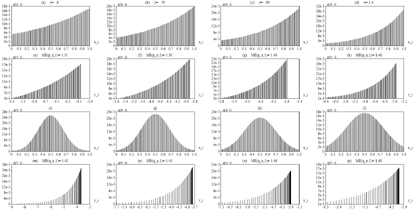
Figure 1: The distributions $p(x_{i})=w\ exp(ci)$ (a-d) and $q(x_{i})=s\ exp(-0.5((ci-\mu)/\sigma)^{2})$ (i-l) as well as their respective transformations $p(y_{i})$ and $q(y_{i}$ for several values of $c$.

Figure 2 depicts the set of alternative moment entropies $\mathrm{FE}(p(x_{i}),k)$ of the distributions $p(x_{i})$ (a) and $q(x_{i})$ (b) as above, in terms of $c$ for several values of $k$, i.e. the order of the alternative entropy moments. The points where the alternative entropy moments of $p(x_{i})$ and $q(x_{i})$ equal one another have been marked by the ‘vertical’ trajectory. It is clear from these results that though the distributions $p$ and $q$ have identical traditional entropy for $c\approx 1.06$, substantial differences are observed between the higher order alternative entropy moments. Interestingly, though the first alternative entropy moment (identical to the traditional entropy) increases with $c$ as expected, the higher order moments tend to decrease with $c$.

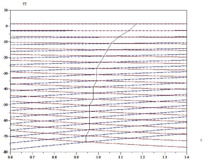
Figure 2: The entropy moments of $p(x_{i})$ (red) and $q(x_{i})$ (blue) in terms of $c$ for several values of $k$ (shown from top to bottom). The firsr upper red and blue upper curves (above 0) correspond to the traditional entropies of $p(x_{i})$ and $q(x_{i})$.

In order to better illustrate the potential of the entropy moments for providing additional information about the original distribution, we now focus our attention on the two above distributions $p(x_{i})$ and $q(x_{i})$ at a value of the parameter $c$ at which they can by no means be discriminated by considering the respective traditional entropies. In order to simulate sampling noise and artifact typically implied while measuring the random variable $x$, we add a uniformly distributed perturbation to each of the two distributions. Figure 3 shows the histograms of the traditional entropies calculated for the two perturbed distributions. Because of the complete superposition between the respective histograms, it is virtually impossible to discriminate between the two cases while taking into account their respective traditional entropies.

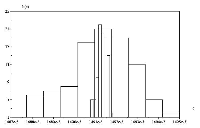
Figure 3: The histograms of the traditional entropy obtained for the perturbed versions of the two distributions $p(x_{i})$ and $q(x_{i})$. Because of the complete overlat between these two histograms, it is completely impossible to discriminate between the original distributions while considering their respective traditional entropies.

We now consider the effect of the consideration of additional entropy moments on the discriminability between the measurements. Figure 4 illustrates the scattering of the entropy moments obtained for the perturbed realizations of the two types of distributions (i.e. $p_{(}x_{i})$ and $q(x_{i})$) considering 3 (a), 6 (b), 9 (c) and 12 (d) entropy moments. The two-dimensional projections shown in Figure 4 were obtained by using the principal component analysis (PCA) methodology (e.g. Duda et al. (2001); Fukunaga (1990); da F. Costa and Cesar (2001)), which ensures maximum dispersion along the first axes of the projections, which are defined by the transformed variables $pca_{i}$, $i=1,2,\ldots$. More specifically, the PCA involves the calculation of the covariance matrix of the considered measurements and estimation of the respective eigenvalues and eigenvectors. The linear transformation used to project the higher dimensional space is defined by the eigenvectors of the covariance matrix taken in decreasing order. In order to compensate for the largely different values of the entropy moments, their values were standardized  prior to the PCA. It is clear from the results shown in Figure 4(a-d) that the incorporation of additional entropy moments contributed substantially for the separation between the perturbed cases. However, the consideration of additional entropy moments tended not to enhance such a separation. For instance, the separation between the two perturbed distributions considering 3 entropy moments (Fig. 4a) is similar to that obtained for 12 entropy moments (Fig. 4d). In addition, the contribution of the higher order entropy moments had almost no effect in increasing the separation between the two categories of observations while considering the third principal component axis, i.e. $pca3$ (see Figs. 4e-h).

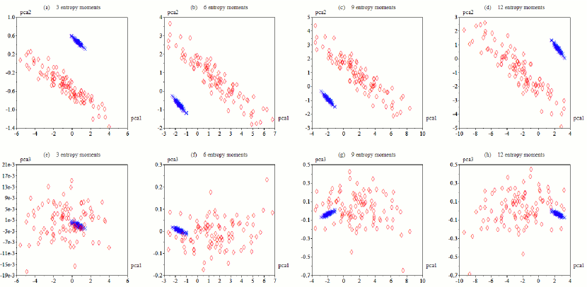
Figure 4: The scattering of the two categories of perturbed distributions as revealed by two-dimensional projection (through PCA) of respective characterizations incorporating 3 (a), 6 (b), 9 (c) and 12 (d) entropy moments.

Figure 5 shows the PCA results considering alternative entropy moments, instead of the entropy moments as above. The incorporation of additional alternative entropy moments allows the increasing discrimination between the two sets of observations regarding all the three first PCA variables (i.e. $pca1$, $pca2$ and $pca3$).

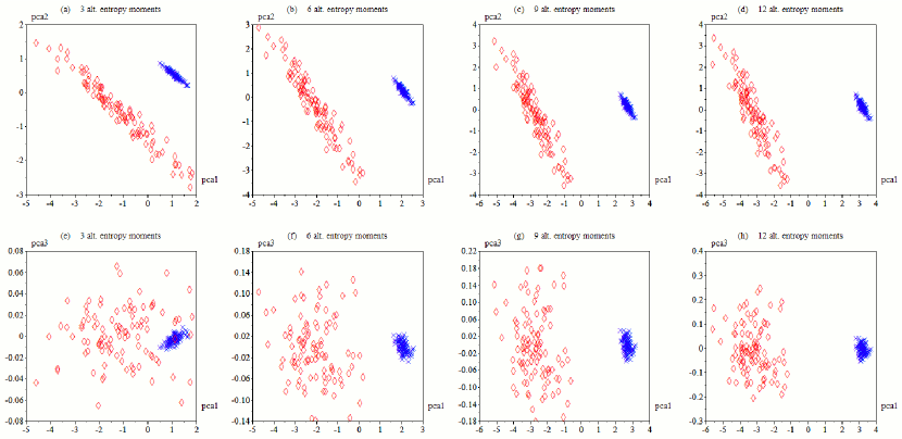
Figure 5: The scattering of the two categories of perturbed distributions as revealed by two-dimensional projection (through PCA) of respective characterizations incorporating 3 (a), 6 (b), 9 (c) and 12 (d) alternative entropy moments.

All in all, we have reported on two families of entropy moments, obtained by interpreting the traditional entropy as the average of a transformed version of the original distribution. Such additional measurements have been shown to contribute substantially for the characterization of the original distributions, as clearly illustrated for a case involving two distributions with undistinguishable traditional entropies. Because of the key role played by entropy in so many areas, the concepts and results described in this work have several immediate implications. Among the several possibilities for future developments, we have the investigation of entropy central moments, including the development of a PCA methodology based on the respectively implied entropy covariance matrix. It would also be interesting to investigate the type of distribution features which lead to extreme values of each of the entropy moments.