A Monte Carlo study of the triangular lattice gas with the first- and the second-neighbor exclusions

Abstract

We formulate a Swendsen-Wang-like version of the geometric cluster algorithm. As an application, we study the hard-core lattice gas on the triangular lattice with the first- and the second-neighbor exclusions. The data are analyzed by finite-size scaling, but the possible existence of logarithmic corrections is not considered due to the limited data. We determine the critical chemical potential as $\mu_{c}=1.75682(2)$ and the critical particle density as $\rho_{c}=0.180(4)$. The thermal and magnetic exponents $y_{t}=1.51(1)\approx 3/2$ and $y_{h}=1.8748(8)\approx 15/8$, estimated from Binder ratio $Q$ and susceptibility $\chi$, strongly support the general belief that the model is in the 4-state Potts universality class. On the other hand, the analyses of energy-like quantities yield the thermal exponent $y_{t}$ ranging from $1.440(5)$ to $1.470(5)$. These values differ significantly from the expected value $3/2$, and thus imply the existence of logarithmic corrections.

I Introduction

Lattice gases, together with the Potts (including Ising) and the O$(n)$ model, play an important role in the statistical mechanics. They are used to describe universal properties of many complex physical systems, ranging from simple fluids to structural glasses and granular materials. Lattice-gas models are generally defined as follows. For a given lattice, a number of particles is randomly distributed over its vertices with the constraint that each vertex can at most be occupied by one particle; the density of particles is controlled by the chemical potential $\mu$. Particles on different vertices can interact with one another–normally through two-body interactions. Accordingly, the reduced Hamiltonian (already divided by $kT$ with Boltzmann factor $k$ and temperature $T$) of a lattice-gas model can be written as

$${\mathcal{H}}=-\mu\sum_{i}\sigma_{i}-K_{1N}\sum_{\{jk\}}\sigma_{j}\sigma_{k}-K_{2N}\sum_{\{lm\}}\sigma_{l}\sigma_{m}+\cdots\;,$$ (1)

where $\sigma=0,1$ represents the absence and the presence of a particle, respectively. The second term with amplitude $K_{1N}$ describes the first-neighbor interactions, and the third one with $K_{2N}$ is for the second-neighbor couplings; further-neighbor interactions can be included, as denoted by symbol $\cdots$.

In the study of lattice gases, one often takes the hard-core limit: in Eq. (1) the couplings $K$ outside a certain range $(r>r_{0})$ are set zero, while $K(r\leq r_{0})$ is taken to the limit $K\rightarrow-\infty$; namely, the particles have a hard-core of radius $r_{0}$. A particular example is the lattice-gas model with nearest-neighbor exclusion: $K_{1N}\rightarrow-\infty$ while all further-neighbor couplings are zero. Unlike the Potts model and the O$(n)$ spin model, the nature and the universality of the phase transitions in lattice-gas systems depend on the lattice structures. For instance, the lattice-gas model with nearest-neighbor exclusions on the square and the honeycomb lattice is believed to be Ising-like, while that on the triangular lattice (Baxter’s hard-hexagon model [1, 2]) belongs to the 3-state Potts universality class.

Extensive investigations have been carried out for lattice gases, and many theoretical and numerical approaches are applied. This includes exact calculations (mainly by Baxter and coauthors), series expansions (like high-temperature and low-temperature expansions), cluster variation method, transfer matrix calculations, and Monte Carlo simulations etc. The critical free energy of Baxter’s hard-hexagon lattice gas was exactly calculated [1, 3, 4, 5]; the critical chemical potential is known as $\mu_{c}=\ln[(11+\sqrt{5})/2]$, and the critical particle density is $\rho_{c}=(5+\sqrt{5})/10$. Baxter’s hard-square model [1, 3, 4, 5], defined by Eq. (1) on the square lattice with $K_{1N}\rightarrow-\infty$ and finite $K_{2N}$, is known to have a tricritical point $(\mu_{tc},K_{2N,tc})$ in the tricritical Ising universality class; the tricritical point lies at $\mu_{tc}=-\ln[8(1+\sqrt{5})]$, $K_{2N,tc}=\ln(3+\sqrt{5})$, with $\rho_{tc}=(5+\sqrt{5})/10$. Using the transfer-matrix technique, Guo and coauthors[6] determine the critical point of the hard-core square lattice gas up to the eleventh decimal place, $\mu_{c}=1.334\,015\,100\,277\,74(1)$, $\rho_{c}=0.367\,742\,999\,041\,0(3)$. Recently, Monte Carlo simulations were carried out for square lattice gases with the hard-core radius up to the fifth neighbors [7]. The nature of phase transitions was found to be continuous for exclusions up to 1N, to 2N, and to 4N, and to be discontinuous for exclusions up to 3N and 5N, where symbols $iN$ represents the $i$th neighbors.

In this work, we shall consider the hard-core lattice gas on the triangular lattice with the first- and the second-neighbor repulsions. The triangular lattice in this case can be divided into four sublattices (see Fig.1), and for sufficiently high density particles prefer to occupying one of the four sublattices. Thus, one would expect that, if it is second order, the melting of ordered phase should be in the 4-state Potts universality class. However, several studies at the end of 60s last century suggested that the phase transition is first order [8, 9]. Later, Bartelt and Einstein [10] reexamined this model by a phenomenological renormalization–transfer-matrix scaling. The largest system size in their study is $16\times\infty$. Slowly convergent finite-size corrections were observed. It was estimated that the thermal and the magnetic critical exponents are $y_{t}=1.400$ and $y_{h}=1.885$, respectively. Despite the noticeable deviations from the exact values $y_{t}=3/2$ and $y_{h}=15/8$ [11, 12], these estimates are in favor of the 4-state Potts universality in view of the possible occurrence of logarithmic corrections.

Here, we aim to provide an independent study of this model by means of Monte Carlo simulations. This seems justified since no rigorous argument exists about the nature of the phase transition and the evidence in Ref. [10] is not very strong. To properly analyze finite-size corrections, more accurate numerical data, particularly for large system sizes, are desirable . Our task becomes now feasible because of the availability of efficient cluster algorithm for lattice-gas models–the geometric cluster algorithm–and the rapid development of computer industry in the past few decades. The geometric cluster algorithm [15, 16] moves round a fraction of particles over the lattice according to geometric symmetries, such as the spatial inversion or rotation symmetries of the triangular lattice; detailed description will be given in Sec. II. The algorithm does not change the total number of particles, and it is combined with the Metropolis steps in order to simulate lattice-gas systems in the grand-canonical ensemble. In comparison with simulations using the Metropolis method only, critical slowing down is significantly suppressed. Therefore, we are able to simulate systems as large as $400\times 400$ within reasonable computer resources.

II Geometric cluster algorithm and sampled quantities

A Geometric cluster algorithm

The geometric cluster algorithm was first proposed by Dress and Krauth [17] in the study of hard-core gases in continuous space. Unlike the well-known Swendsen-Wang (SW) cluster method which flips spins, the elementary operation in this algorithm is to move particles. For hard disks, the percolation threshold of the cluster formation process deviates significantly from the phase transition of the model. This is unfortunate since it affects the efficiency of the algorithm.

A single-cluster version of the geometric cluster algorithm was later developed by Heringa and Blöte [15, 16] for lattice models like the Potts model and the lattice gases. Here, we shall briefly describe it in terms of the lattice-gas model (1) with a soft-core radius of a lattice unit (finite $K:\equiv K_{1N}<0$ and all other couplings are zero) on the square lattice with periodic boundary conditions. For such a geometry, one can set a Cartesian coordinate by taking any two perpendicular lines of lattice sites as the $x$ and the $y$ axis, respectively. It can be seen that the Hamiltonian of the system is invariant under geometric operations like reflections about the $x$ or the $y$ axis or inversion about the center of the coordinate. Further, any configuration will be restored if an operation is subsequently applied twice–namely, these operations are self-inverse. One can employ any of such geometric operations to formulate a cluster algorithm. Let a pair of nearest-neighboring sites $i,k$ be mapped onto $i^{\prime},k^{\prime}$, respectively. One denotes the energy difference when a neighbor $k$ of $i$ is interchanged with $k^{\prime}$ as $\Delta_{ik}$, which is $\Delta_{ik}=K(\sigma_{i}\sigma_{k}+\sigma_{i^{\prime}}\sigma_{k^{\prime}}-\sigma_{i}\sigma_{k^{\prime}}-\sigma_{i^{\prime}}\sigma_{k}$). The algorithm then involves the following steps:

1. Choose a random site $i$: both $i$ and $i^{\prime}$ belong to the cluster.

2. Interchange $\sigma_{i}$ and $\sigma_{i^{\prime}}$.

3. For all neighbors $k$ of $i$ that do not belong to the cluster yet, do the following:

   • If $\Delta_{ik}>0$, do the following with probability $p=1-\exp(-\Delta_{ik})$: (a) interchange $\sigma_{k}$ and $\sigma_{k^{\prime}}$ ($k$ and $k^{\prime}$ are included in the cluster), (b) write $k$ in a list of addresses (called the stack).

   • If $\Delta_{ik}<0$, do nothing.

4. Read an address $j$ from the stack. Substitute $j$ for $i$, and execute Step 3.

5. Erase $j$ from the stack.

6. Repeat Steps 4 and 5 until the stack is empty.

When the stack is empty, the cluster is completed. Since the elementary operation is to interchange spins $\sigma_{i}$ and $\sigma_{i^{\prime}}$, the total number of particles does not change in the algorithm.

For the above geometric cluster steps, the detailed balance has already been proved[15, 16]. The efficiency of this algorithm for different models has also been demonstrated. For the Ising model, it was shown that the percolation of the formed clusters coincides with the thermal phase transition, reflecting the efficiency of the algorithm. In fact, in the canonical ensemble (the total number of particles is fixed), it can be shown that, for many models, no critical slowing down exist for some quantities [18].

Here we shall formulate a full-cluster version of the geometric cluster algorithm in an analogous way as the Edward-Sokal picture for the well-known SW cluster method for the ferromagnetic Potts model [19, 20]. We consider the lattice-gas model (1) with finite nearest-neighbor interactions ($K:\equiv K_{1N}<0$) on a one-dimensional chain with sites labelled as $i=\pm 1/2,\pm 3/2,\pm 5/2,\cdots$. Instead of writing the Hamiltonian for a fixed number of particles as a sum of the nearest-neighbor couplings like in Eq. (1), we rewrite it as

$${\mathcal{H}}|_{N_{p}=N}=\sum_{i=1/2}^{\infty}{\mathcal{H}}_{i}=-K\sum_{i=1/2}^{\infty}(\sigma_{i}\sigma_{i+1}+\sigma_{-i}\sigma_{-i-1}),$$ (2)

where $N_{p}=\sum_{i}\sigma_{i}$ and the constant $N$ denotes the total number of particles. The Hamiltonian (2) is obtained by applying the reflection about the center $i=0$–a geometric operation. In this form, the ‘building blocks’ of the Hamiltonian is no longer a pair of neighboring sites, but two pairs of them. If one only uses the spin-interchange operation $\eta:\equiv\sigma_{i}\leftrightarrow\sigma_{-i}$, the energy associated with each building block is of two levels at most: ${\mathcal{E}}_{1}(\vec{\sigma}):\equiv-K(\sigma_{i}\sigma_{i+1}+\sigma_{-i}\sigma_{-i-1})$ and ${\mathcal{E}}_{2}(\vec{\sigma}):\equiv-K(\sigma_{i}\sigma_{-i-1}+\sigma_{-i}\sigma_{i+1})$. The former ${\mathcal{E}}_{1}$ refers to the status that no operator $\eta$ is applied or it is applied at both vertices $i$ and $j$; instead, the latter ${\mathcal{E}}_{2}$ means that $\eta$ is applied at $i$ (or $j$) only. The values of ${\mathcal{E}}_{1}$ and ${\mathcal{E}}_{2}$ depend on the spin configuration $\vec{\sigma}$ on the building block. For the lattice-gas mode (2), these values are shown in Table I. Let us denote the lower and the upper level of ${\mathcal{E}}_{1}$ and ${\mathcal{E}}_{2}$ as ${\mathcal{E}}_{\rm low}$ and ${\mathcal{E}}_{\rm upp}$, respectively. The statistical weight associated with each block in Eq. (2) reads

$$e^{-{\mathcal{H}}_{i}(\vec{\sigma})}=e^{-{\mathcal{E}}_{\rm upp}}(1+v_{i}\delta_{{\mathcal{E}}_{1},{\mathcal{E}}_{\rm low}})\hskip 28.45274pt\mbox{with}\hskip 5.69054pt(v_{i}=e^{{\mathcal{E}}_{\rm upp}-{\mathcal{E}}_{\rm low}}-1).$$ (3)

On this basis, the partition sum becomes

$${\mathcal{Z}}|_{N_{p}=N}=\sum_{\{\sigma\}:N_{p}=N}\;\;\prod_{i=1/2}^{\infty}e^{-{\mathcal{E}}_{\rm upp}(\vec{\sigma})}\prod_{i=1/2}^{\infty}(1+v_{i}\delta_{{\mathcal{E}}_{1},{\mathcal{E}}_{\rm low}}).$$ (4)

Analogously as mapping the Potts model onto the random-cluster model, one introduces a bond variable $b_{i}$ to graphically represent the expansion of the second product in Eq. (4): if the term $v_{i}\delta_{{\mathcal{E}}_{1},{\mathcal{E}}_{\rm low}}$ is taken, an occupied bond $b_{i}=1$ is placed between sites $i$ and $i+1$; otherwise, no bond is placed ($b_{i}=0$). This leads to a joint model

$${\mathcal{Z}}|_{N_{p}=N}=\sum_{\{\sigma\}:N_{p}=N}\;\;\prod_{i=1/2}^{\infty}e^{-{\mathcal{E}}_{\rm upp}(\vec{\sigma})}\sum_{\{b\}}(v_{i}\delta_{{\mathcal{E}}_{1},{\mathcal{E}}_{\rm low}})^{b_{i}},$$ (5)

where the second sum is over all possible bond configurations that are consistent with the spin configuration, and we have already assumed the conventional symbol $0^{0}=1$. Given a spin configuration $\{\sigma\}$, the expression (5) allows us to place bonds and construct clusters as follows: if the spin configuration on a block $i$ is at the lower-energy level ${\mathcal{E}}_{\rm low}$, one places a bond $b_{i}=1$ with probability $v_{i}/(1+v_{i})$; otherwise, place no bonds. Note that a bond connects four lattice sites, since it is placed on the blocks. Lattice sites connected through a chain of occupied bonds form a cluster. The condition $\delta_{{\mathcal{E}}_{1},{\mathcal{E}}_{\rm low}}=1$ for a block can be hold either by doing nothing or interchanging both spins ($\sigma_{i}\leftrightarrow\sigma_{-i},\sigma_{i+1}\leftrightarrow\sigma_{-i-1}$). Thus, for a spin-jointed-bond configuration, for each cluster one has the freedom to choose the do-nothing or the spin-interchange operation, and apply it to all lattice sites within the cluster. Accordingly, a Swendsen-Wang-like geometric cluster algorithm can be formulated as follows.

1. Choose a geometric transformation such that every building block in the Hamiltonian consists of two pairs of neighboring couplings and the associated energy is only of two levels under the spin-interchange operation.

2. For each building block $i$ (containing four lattice sites), if its spin configuration is at the lower-energy ${\mathcal{E}}_{\rm low}$, place a bond with probability $p_{i}=v_{i}/(1+v_{i})$; otherwise, place no bond.

3. Construct clusters according to the occupied bonds.

4. Independently for each cluster, randomly choose the do-nothing or the spin-interchange operation with probability $1/2$; apply the chosen operation to all lattice sites within the cluster.

A Monte Carlo step is completed, and a new spin configuration is obtained. We expect that the analogy between our formulation of the geometric cluster algorithm and the well-known SW method can help the reader to understand the geometric cluster algorithm.

We conclude this subsection by mentioning the following. (1), like the SW method, the essence in the geometric cluster process is that the energy of each building block has two levels only under the spin-interchange operation (the energy of a building block may have more than two levels if other operations–like the spin-flip operation–are allowed). (2), normally, the rewriting of the Hamiltonian as a sum of proper building blocks is obtained by applying some global geometric transformation, such as the inversion about the center and reflection etc. (3), in the canonical ensemble, if one uses the geometric cluster algorithm only, a large number of spatial transformations should be available such that each lattice site in a system should be able to reach any other lattice site by a finite number of geometric mappings. For the torus geometry, this can be easily achieved since any site can serve as the center of the aforementioned Cartesian coordinate. In case that the geometric cluster method is itself non-ergodic, it can be combined with other algorithms like the Kawasaki dynamic. (4), for simulations in the grand-canonical ensemble, other Monte Carlo methods have to be used.

B Sampled quantities

For the lattice-gas model (1), the triangular lattice is divided into four sublattices. The particle density is then sampled as

$$\rho^{(i)}=\frac{4}{V}\sum_{k\in{\mathcal{T}}^{(i)}}\sigma_{k}$$ (6)

where $V=L\times L$ is the volume of the lattice and the sum is over each sublattice, labelled as $i=1,2,3,4$. The global particle density is then $\rho=(\rho^{(1)}+\rho^{(2)}+\rho^{(3)}+\rho^{(4)})/4$. On this basis, we measured the second and the fourth moment of the magnetization density as

$${\mathcal{M}}^{2}=\frac{1}{3}\sum_{i=1}^{3}\sum_{j=i+1}^{4}(\rho^{(i)}-\rho^{(j)})^{2}\hskip 28.45274pt\mbox{and}\hskip 28.45274pt{\mathcal{M}}^{4}=\left({\mathcal{M}}^{2}\right)^{2}\;,$$ (7)

where factor $1/3$ is for normalization purpose such that ${\mathcal{M}}^{2}$ is a unity when the chemical potential is infinite–one of the four sublattices is fully occupied. The magnetic susceptibility is $\chi=V\langle{\mathcal{M}}^{2}\rangle$. Then, we define a dimensionless ratio as

$$Q=\frac{\langle{\mathcal{M}}^{2}\rangle^{2}}{{\langle\mathcal{M}}^{4}\rangle}\,.$$ (8)

This ratio at criticality approaches a universal value for $L\rightarrow\infty$, and is known to be very useful in estimating critical points.

Since a pair of first- (or second-) neighboring sites cannot be both occupied by particles, we sampled the third-neighbor correlation as an energy-like quantity

$${\mathcal{E}}=\frac{1}{6V}\sum_{\{ij\}\in 3N}\sigma_{i}\sigma_{k}$$ (9)

where the sum is over all the third-neighbor pairs. Correspondingly, a specific-heat-like quantity is defined as ${\mathcal{C}}_{e}=V(\langle{\mathcal{E}}^{2}\rangle-\langle{\mathcal{E}}\rangle^{2})$. We also measured the compressibility ${\mathcal{C}}_{v}=V(\langle\rho^{2}\rangle-\langle\rho\rangle^{2})$.

III Results

Using a combination of the Metropolis and the geometric cluster algorithm, we simulated the lattice-gas model on the triangular lattice with first- and second-neighbor repulsions. Periodic boundary conditions were used in the rhombus geometry shown in Fig. 1. System sizes took 15 values in range $8\leq L\leq 400$. Several geometric cluster steps are performed between subsequent Metropolis steps. such that the total number of particles moved by the former is also approximately equal to $V$. Significant critical slowing down was observed, with a dynamic exponent about $z\approx 1$.

Some primary simulations for relatively small system sizes were first carried out to find the approximate location of the critical point from the intersection of the $Q$ data for different system sizes $L$ (we were also guided by the result $\mu_{c}\approx 1.7599$ in Ref. [10]). Then extensive simulations for large sizes were performed near $\mu_{c}=1.757$.

Figure 2 shows parts of the Monte Carlo data of the dimensionless ratio $Q$. According to the least-squares criterion, the $Q$ data were fitted by

$$Q(\mu,L) = Q_{c}+q_{1}(\mu-\mu_{c})L^{y_{t}}+q_{2}(\mu-\mu_{c})L^{2y_{t}}$$ (11)

$$+b_{1}L^{y_{1}}+b_{2}L^{y_{2}}+b_{3}L^{y_{3}}+r_{1}L^{y_{r}}+c_{1}(\mu-\mu_{c})L^{y_{t}+y_{1}}\;,$$

where $q_{i}$ , $b_{i}$ , $c_{i}$ , and $r_{i}$ are unknown parameters, and $Q_{c}$ is the universal value. The terms with $q_{i}$ describe the contributions of the thermal field due to deviation from the critical point, those with exponent $y_{i}$ account for finite-size corrections, and the one with $c_{1}$ is for the mixed effect of the relevant and irrelevant thermal fields. The term with exponent $y_{r}=d-2y_{h}$ arises from the regular part of the free energy, where the magnetic exponent $y_{h}$ was fixed at $15/8$ for the four-state Potts model. The detailed derivation of the finite-size scaling formula (11) can be found in Ref. [14]. In principle, one should include logarithmic corrections in Eq.(11) [21], since the transition is expected to be in the 4-state Potts universality class. Unfortunately, the limited system size does not allow us to include such corrections (accordingly, the statistical error margins of our following results should be taken carefully). From the numerical results for the tricritical 4-state Potts model [18] where the marginal field is absent, we learn that there exist correction terms with exponent $y_{1}=-1$. Thus, we set $y_{1}=-1$, $y_{2}=-2$, and $y_{3}=-3$. Satisfactory fits can be obtained after a cutoff for small system sizes $L<18$, which yield $\mu_{c}=1.75682(2)$, $y_{t}=1.51(1)\approx 3/2$ and $Q_{0}=0.823(2)$. It is interesting to observe that, without logarithmic corrections, satisfactory fits can include data for rather small sizes and the exponent $y_{t}=1.51(1)$ agrees well with the exact value $3/2$. This suggests that logarithmic corrections are small in the $Q$ data, and thus the fitting results for $Q$ are more or less reliable.

We then fitted the $\chi$ data by

$$\chi = \chi_{0}+L^{2y_{h}-2}[a_{0}+a_{1}(\mu-\mu_{c})L^{y_{t}}+a_{2}(\mu-\mu_{c})L^{2y_{t}}$$ (12)

$$+ b_{1}L^{y_{1}}+b_{2}L^{y_{2}}+c_{1}(\mu-\mu_{c})L^{y_{t}+y_{1}}]\;,$$ (13)

where $\chi_{0}$ stems from the regular part of the free energy, which acts in Eq. (11) as a correction term with exponent $y_{r}=2-2y_{h}$. The correction exponents were also set as $y_{1}=-1$ and $y_{2}=-2$. After a cutoff for small systems $L<20$, we obtain $\mu_{c}=1.75683(1)$ , $y_{t}=1.489(9)\approx 3/2$ and $y_{h}=1.8748(8)\approx\frac{15}{8}$. The estimate of $\mu_{c}$ is consistent with that from $Q$, and those for $y_{t}$ and $y_{h}$ agree with the exact values. If the exponent $y_{t}$ is fixed at $3/2$, one has $\mu_{c}=1.75683(1)$ and $y_{h}=1.8743(7)$ after discarding the data for $L<18$.

The data for the particle density $\rho$ were fitted by

$$\rho = \rho_{0}+\rho_{1}(\mu-\mu_{c})+L^{y_{t}-d}[a_{0}+a_{1}(\mu-\mu_{c})L^{y_{t}}+a_{2}(\mu-\mu_{c})L^{2y_{t}}$$ (15)

$$+b_{1}L^{-1}+b_{2}L^{-2}+b_{3}L^{-3}]\;.$$

Satisfactory fits are obtained after a cutoff for small systems $L<16$, and we have $\mu_{c}=1.75682(2)$ , $y_{t}=1.440(5)$ and $\rho_{c}=0.180(4)$. The result $\mu_{c}=1.75680(3)$ agrees well with those obtained from magnetic quantities $Q$ and $\chi$. However, the value $y_{t}=1.440(5)$ significantly differs from $3/2$. This might imply that, while additive logarithmic corrections are still small in energy-like quantities, multiplicative logarithmic corrections cannot be neglected.

The finite-size scaling formula of the specific-heat-like quantities $C_{e}$ and $C_{v}$ reads

$$C = r_{0}+r_{1}(\mu-\mu_{c})+L^{2y_{t}-d}[a_{0}+a_{1}(\mu-\mu_{c})L^{y_{t}}+a_{2}(\mu-\mu_{c})L^{2y_{t}}+a_{3}(\mu-\mu_{c})L^{3y_{t}}$$ (17)

$$+b_{1}L^{-1}+b_{2}L^{-2}+b_{3}L^{-3}+c_{1}L^{y_{t}-1}(\mu-\mu_{c})]\;.$$

In the actual fits, the terms $r_{0}$, arising from the regular part of free energy, cannot be distinguished from the correction term $b_{1}L^{2y_{t}-d-1}=b_{1}$, and so is for $r_{1}$ and $c_{1}$. Thus, we simply set $r_{0}$ and $r_{1}$ to be zero. The data for $L\geq 18$ are well described by Eq. (17). The fits for $C_{v}$ yield $\mu_{c}=1.75682(3)$ , $y_{t}=1.468(7)$ and those for $C_{e}$ yield $\mu_{c}=1.75680(2)$ , $y_{t}=1.470(5)$. Again, the estimates of $\mu_{c}$ agree well with those from other quantities, while the values of $y_{t}$ differ significantly from $3/2$.

We have simulations at $\mu=1.756818$, at criticality within the estimated error bars. Thus, we could analyze various quantities right at the critical point. The finite-size scaling behavior of $\chi$, $\rho$, and $C_{e}$ and $C_{v}$ at criticality is given by Eqs. (13), (15), and (17), respectively, by throwing out those $\mu$-dependent terms. The estimates of the associated critical exponents from these simplified analyses are consistent with those from the aforementioned fits. Figures 3 and 4 show the critical $\chi$ and $C_{e}$ data, respectively.

IV Discussion

In the language of the lattice gas systems, we formulate a Swendsen-Wang-like version of the geometric cluster algorithm that has already found many applications [18, 22]. Since our formulation is in line with the Swendsen-Wang algorithm for the ferromagnetic Potts model, we expect that it will help the reader to understand the geometric cluster method.

We then study the triangular lattice gases with the first- and the second-neighbor exclusion, using a combination of the Metropolis and the geometric cluster algorithm. The estimated critical point $\mu_{c}=1.75682(2)$ significantly improves over the existing result $1.7599$; to our knowledge, no report has been published yet for the critical particle density $\rho_{c}=0.180(4)$. The excellent agreement between the exact values and the numerical estimates $y_{t}=1.51(1)$ and $y_{h}=1.8743(7)$ give strong support for the expectation that the model is in the 4-state Potts universality class. On the other hand, the fitting results from energy-like quantities imply that, although additive logarithmic corrections might be small, multiplicative logarithmic corrections cannot be neglected at least in energy-like quantities.

The fitting results are summarized in Table II.

Acknowledgements This work was partially supported by the National Natural Science Foundation of China under Grant No. 10447111 and the Alexander von Humboldt Foundation of Germany (YD). One of us (YD) is greatly indebted to Henk W.J. Blöte, Timothy G. Garoni, and Alan D. Sokal for valuable discussions.

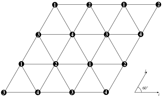
FIG. 1.: The triangular lattice and its four sublattices. For chemical potential $\mu\rightarrow\infty$, one of the sublattices is fully occupied.

FIG. 2.: Ratio $Q$ versus $\mu$ for various system sizes. The straight line segments, simply connecting the data points, are for illustration purpose.

FIG. 3.: Quantity $\chi/L^{2}$ at $\mu=1.756818$ versus $L^{2y_{h}-4}$, with $y_{h}=15/8$. The statistical error bars are smaller than the size of the data points. The dashed line is just for illustration purpose.

FIG. 4.: Specific-heat-like quantity $C_{e}$ at $\mu=1.756818$ versus $L^{2y_{t}-2}$, where the value of $y_{t}=1.470$ is taken form the fit. The statistical error bars of the data points are in the same order of their size. The dashed line is for illustration purpose.

TABLE I.: Energies ${\mathcal{E}}_{1}$ and ${\mathcal{E}}_{2}$ of a building block in Eq. (2). The associated bond weight for $K<0$ in the geometric cluster algorithm is also given. In the “Example”, the upper two sites are $i$ and $i+1$, and the lower are $-i$ and $-i-1$. The filled (empty) circle represents the presence (absence) of a particle.

Case	1	2	3	4	5	6	7
	0 particle	1 particle	2 particles			3 particles	4 particles
Example	$\circ$–$\circ$	$\bullet$–$\circ$	$\bullet$–$\circ$	$\bullet$–$\bullet$	$\bullet$–$\circ$	$\bullet$–$\bullet$	$\bullet$–$\bullet$
	$\circ$–$\circ$	$\circ$–$\circ$	$\bullet$–$\circ$	$\circ$–$\circ$	$\circ$–$\bullet$	$\bullet$–$\circ$	$\bullet$–$\bullet$
${\mathcal{E}}_{1}$	0	0	0	$-K$	0	$-K$	$-2K$
${\mathcal{E}}_{2}$	0	0	0	0	$-K$	$-K$	$-2K$
$v$	0	0	0	0	$e^{-K}-1$	0	0

TABLE II.: Fitting results for various quantities. Symbol $L_{\rm min}$ is the minimum system size for which the Monte Carlo data are included in the fit.

Quantity	$L_{min}$	$\mu_{c}$	$\rho_{c}$	$y_{t}$	$y_{h}$
$Q$	$20$	$1.75682(2)$		$1.51(1)$
$\chi$	$20$	$1.75683(1)$		$1.489(9)$	$1.8748(8)$
$\rho$	$18$	$1.75680(3)$	$0.180(4)$	$1.440(5)$
${\mathcal{E}}$	$12$	$1.75680(2)$		$1.48(2)$
$C_{e}$	$18$	$1.75680(2)$		$1.470(5)$
$C_{v}$	$18$	$1.75682(3)$		$1.468(7)$
Previous		$1.7599$		$1.400$	$1.885$

REFERENCES

- [1] R.J. Baxter, J. Phys. A 13,L61 (1980).
- [2] R.J. Baxter, Exactly Solved Models in Statistical Mechanics Academic Press Inc. San Diego, CA 92101, 1982.
- [3] R.J. Baxter, J. Stat. Phys. 26, 427 (1981).
- [4] D.A. Huse, Phys. Rev. Lett. 49, 1121 (1982).
- [5] R.J. Baxter and P.A. Pearce, J. Phys. A 16, 2239 (1983).
- [6] W. Guo and H.W.J. Blöte, Phys. Rev. E 66, 046140 (2002).
- [7] H.C.M. Fernandes, J.J. Arenzon and Y. Levinn, J. Chem. Phys. 126, 114508 (2007).
- [8] J. Orban and A. Bellemans, J. Chem. Phys. 49, 363 (1968)
- [9] L.K. Runnels, J.R. Craig, and H.R. Stereiffer, J. Chem. Phys. 54, 2004 (1971)
- [10] N.C. Bartelt and T.L. Einstein, Phys. Rev. B 30, 5339 (1984).
- [11] B. Nienhuis, Phase Transitions and Critical Phenomena, edited by C. Domb and J.L. Lebowitz. (Academic Press, London, 1987), Vol. 11, p 1, and references therein.
- [12] J.L. Cardy, Phase Transitions and Critical Phenomena, edited by C. Domb and J.L. Lebowitz. (Academic Press, London, 1987), Vol. 11, p. 55, and references therein.
- [13] A. Yamagata, Physica A 222, 119 (1995); 231, 495 (1996).
- [14] Y. Deng and H.W.J. Blöte, Phys. Rev. E 68, 036125 (2003).
- [15] J.R. Heringa and H.W.J. Blöte, J. Phys. A 232, 369-374 (1996).
- [16] J.R. Heringa and H.W.J. Blöte, Phys. Rev. E 57, 5 (1998).
- [17] C. Dress and W. Krauth, J. Phys. A 28, L597 (1995).
- [18] Y. Deng, J.R. Heringa, and H.W.J. Blöte, Phys. Rev. E 71, 036115 (2005); Y. Deng and H.W.J. Blöte, 70, 046111 (2004).
- [19] R.H. Swendsen and J.S. Wang, Phys. Rev. Lett. 58, 86 (1987).
- [20] R.G. Edwards and A.D. Sokal, Phys. Rev. D 38, 2009 (1988)
- [21] J. Salas and A.D. Sokal, J. Stat. Phys. 88, 567-615 (1997)
- [22] J.W. Liu and E. Luijten, Phys. Rev. Lett. 93, 247802 (2004); Phys. Rev. E 71, 066701 (2005).