Chiral Corrections and the Axial Charge of the Delta

Abstract

Chiral corrections to the delta axial charge are determined using heavy baryon chiral perturbation theory. Knowledge of this axial coupling is necessary to assess virtual-delta contributions to nucleon and delta observables. We give isospin relations useful for a lattice determination of the axial coupling. Furthermore we detail partially quenched chiral corrections, which are relevant to address partial quenching and/or mixed action errors in lattice calculations of the delta axial charge.

Introduction.— Numerical simulations of QCD on spacetime lattices provide a first principles method to study non-perturbative regime of QCD DeGrand and DeTar (2006). For the last decade, lattice QCD has made dramatic progress due to enlarged computing resources, and advances in numerical algorithms. Even with considerable progress, lattice simulations are still restricted to unphysically large quark masses, and lattice sizes that are not much larger than typical hadronic length scales. Fortunately, low-energy hadronic physics is dominated by pion interactions which can be studied systematically using chiral perturbation theory ($\chi$PT). Today lattice data in conjunction with $\chi$PT enable first principles predictions, and in turn, the investigation of the low-energy effective theory.

Properties of baryons can be addressed systematically using $\chi$PT Jenkins and Manohar (1991a, b). There are, however, notable complications to this proposal. The number of a priori unknown low-energy constants for baryons is larger at next-to-leading order compared to those of mesons. The chiral expansion in powers of $m_{\pi}^{2}/\Lambda_{\chi}^{2}$, where $m_{\pi}$ is the pion mass and $\Lambda_{\chi}$ the chiral symmetry breaking scale, is accompanied by an expansion in $m_{\pi}/M_{N}$, where $M_{N}$ is the nucleon mass in the chiral limit. Finally the nearby delta-resonances can lead to important contributions. For a recent review of delta physics, see Pascalutsa et al. (2007). The axial charge of the nucleon, for example, receives important virtual contributions from pion-delta intermediate states because the delta-nucleon mass splitting is about the same size as the pion mass, and the axial couplings $G_{{\Delta}N}$, and $G_{{\Delta}{\Delta}}$ are of order one. We focus on the axial charge of the delta, $G_{{\Delta}{\Delta}}$. The value of this parameter is largely unknown for two reasons. Firstly and obviously, the short mean lifetime of the delta complicates experimental extraction of this coupling. Secondly the value of $G_{{\Delta}{\Delta}}$ has been inferred from one-loop chiral computations of various baryon observables. These computations are incomplete, however, as they only roughly estimate or completely neglect local contributions from unknown low-energy constants. There are too many unknowns to extract reliable information about $G_{{\Delta}{\Delta}}$ from chiral computations alone. Lattice QCD simulations can remedy this.

Early work on the delta using lattice QCD centered on electromagnetic moments and delta-to-nucleon electromagnetic transitions Leinweber et al. (1992, 1993). These calculations have been refined recently Alexandrou et al. (2005); Alexandrou et al. (2007a, b), by including the effects of dynamical quarks, and reaching much lower pion masses $\sim 350\,\texttt{MeV}$. The axial nucleon-to-delta transition has also been studied on the lattice for the first time Alexandrou et al. (2007c, d). The delta axial charge, $G_{{\Delta}{\Delta}}$, can also be determined using lattice QCD. A necessarily component for this study is the stability of the delta. Above the decay threshold, $m_{\pi}>{\Delta}$, where ${\Delta}$ is the delta-nucleon mass splitting in the chiral limit, the delta will be a stable particle on the lattice. Its static properties can be calculated and the effective theory is used, in turn, to extrapolate down to the physical point, where the axial matrix element becomes complex valued. Lighter pion masses too can be employed. The reason being that the delta decays via $p$-wave pion emission, and the available momentum modes are restrictive enough to keep the delta lattice stabilized. Lattice study of the delta at lighter pion masses requires more care, especially with volume effects Bernard et al. (2007), but could better control the chiral expansion of delta properties.

In this work, we relate various delta matrix elements to the axial coupling $G_{{\Delta}{\Delta}}$. The connected ${\Delta}^{++}$ matrix element provides a convenient starting point for lattice simulations. We compute the one-loop chiral corrections to the delta axial charge, and investigate its pion mass dependence. The modulus $|G_{{\Delta}{\Delta}}|$ is shown to be relatively stable with respect to chiral corrections. Finally we perform the partially quenched chiral computation.

Delta Axial Matrix Elements.— There are various axial current matrix elements in the quartet of $\Delta$-resonances. Several of these can be used at zero momentum transfer to define the axial charge, $G_{{\Delta}{\Delta}}$. The remaining choices are then completely determined as a product of $G_{{\Delta}{\Delta}}$ and isospin Clebsch-Gordan coefficients. To arrive at the conventional definition, we define the axial charge through the relation

$$\langle{\Delta}^{++}|J^{3}_{\mu 5}|{\Delta}^{++}\rangle-\langle{\Delta}^{-}|J^{3}_{\mu 5}|{\Delta}^{-}\rangle=G_{{\Delta}{\Delta}}\mathcal{M}_{\mu},$$ (1)

in which appears the axial current $J_{\mu 5}^{a}={\overline{Q}}\gamma_{\mu}\gamma_{5}T^{a}Q$ , where the isospin generators are given by $T^{a}=\frac{1}{2}\tau^{a}$, with $\tau^{a}$ as Pauli matrices. The factor $\mathcal{M}_{\mu}$ encodes the spin structure of the forward matrix element, namely $\mathcal{M}_{\mu}={\overline{U}}{}^{\nu}(P)\gamma_{\mu}\gamma_{5}U_{\nu}(P)$, where $U_{\nu}(P)$ is a Rarita-Schwinger spinor. The definition in Eq. (1) can be easily utilized to calculate $G_{{\Delta}{\Delta}}$ on the lattice. Because differences of isosinglet matrix elements vanish, we can write Eq. (1) as

$$\langle{\Delta}^{++}|{\overline{u}}\gamma_{\mu}\gamma_{5}u|{\Delta}^{++}\rangle_{\text{conn.}}=G_{{\Delta}{\Delta}}\mathcal{M}_{\mu},$$ (2)

where the subscript denotes only connected quark contractions.

For completeness, we specify the other matrix elements from which the axial charge can be deduced. The isospin changing matrix elements are related by the Wigner-Eckart theorem. We consider only ${\Delta}I=+1$ for ease, and find

$$\langle{\Delta}^{++}|J^{+}_{\mu 5}|{\Delta}^{+}\rangle = \frac{1}{\sqrt{3}}C\mathcal{M}_{\mu}$$

$$\langle{\Delta}^{+}|J^{+}_{\mu 5}|{\Delta}^{0}\rangle = \frac{2}{3}C\mathcal{M}_{\mu}$$

$$\langle{\Delta}^{0}|J^{+}_{\mu 5}|{\Delta}^{-}\rangle = \frac{1}{\sqrt{3}}C\mathcal{M}_{\mu},$$ (3)

where $C$ is proportional to the common reduced matrix element. Using isospin, one can relate the isospin transitions to differences of ${\Delta}I=0$ matrix elements and thus leads to

$$\frac{1}{\sqrt{3}}\langle{\Delta}^{++}|J^{+}_{\mu 5}|{\Delta}^{+}\rangle = \langle{\Delta}^{++}|J^{3}_{\mu 5}|{\Delta}^{++}\rangle-\langle{\Delta}^{+}|J^{3}_{\mu 5}|{\Delta}^{+}\rangle$$

$$\frac{1}{2}\langle{\Delta}^{+}|J^{+}_{\mu 5}|{\Delta}^{0}\rangle = \langle{\Delta}^{+}|J^{3}_{\mu 5}|{\Delta}^{+}\rangle-\langle{\Delta}^{0}|J^{3}_{\mu 5}|{\Delta}^{0}\rangle$$

$$\frac{1}{\sqrt{3}}\langle{\Delta}^{0}|J^{+}_{\mu 5}|{\Delta}^{-}\rangle = \langle{\Delta}^{0}|J^{3}_{\mu 5}|{\Delta}^{0}\rangle-\langle{\Delta}^{-}|J^{3}_{\mu 5}|{\Delta}^{-}\rangle.$$

Combining all three of these relations shows that $C=G_{{\Delta}{\Delta}}$. One can then utilize the ${\Delta}I=1$ relations in Eq. (3) to determine the axial charge, or the matrix element differences in Eq. (LABEL:eq:Differences). The former are directly tied to weak interaction phenomenology, while the latter are straightforward to implement on the lattice, e.g., Eq. (2). As with the other baryon axial couplings, there are no disconnected diagrams to evaluate. When we generalize to partially quenched theories (or additionally mixed lattice actions), the above relations between matrix elements remain valid because of the vector isospin symmetry in the valence sector.

Chiral Computations.— The $SU(2)_{L}\otimes SU(2)_{R}$ symmetry of two-flavor QCD is spontaneously broken down to the vector subgroup. The low-energy dynamics are described by pseudo-Goldstone pions emerging from spontaneous chiral symmetry breaking. These modes, $\phi$, are non-linearly realized in the coset field $\Sigma\equiv\xi^{2}=\exp(2i\phi/f)$, where

$$\phi=\begin{pmatrix}\pi^{0}/\sqrt{2}&\pi^{+}\\ \pi^{-}&-\pi^{0}/\sqrt{2}\end{pmatrix},$$ (5)

and $f=132\,\texttt{MeV}$ is the pion decay constant. Pion dynamics are described at leading order by the effective Lagrangian

$${\mathcal{L}}=\frac{f^{2}}{8}\text{tr}(\partial^{\mu}\Sigma^{\dagger}\partial_{\mu}\Sigma)+\frac{f^{2}m_{\pi}^{2}}{8}\text{tr}(\Sigma^{\dagger}+\Sigma).$$ (6)

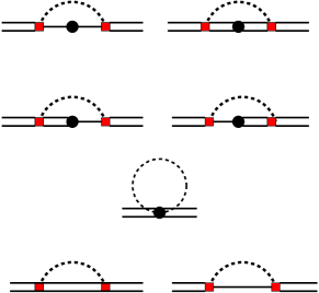
Figure 1: One-loop diagrams which contribute non-analytic terms to the axial charge of the delta. Mesons are represented by a dashed line, while the single and double lines are the symbols for nucleons and deltas respectively. The solid circle is an insertion of the axial current operator. The wave function renormalization diagrams are shown at the bottom.

The baryons are contained in $SU(2)_{V}$ multiplets: a doublet $N$ of spin-$1/2$ nucleons and a quartet $T$ of spin-$3/2$ deltas. The Lagrangian up to NLO describing the nucleons, deltas and their interactions with pions is given by

$${\mathcal{L}} = i{\overline{N}}v\cdot DN-i{\overline{T}}_{\mu}v\cdot DT^{\mu}+{\Delta}{\overline{T}}_{\mu}T^{\mu}+2g_{A}{\overline{N}}S\cdot AN$$ (7)

$$+ g_{{\Delta}N}\left({\overline{T}}_{\mu}A^{\mu}N+{\overline{N}}A_{\mu}T^{\mu}\right)+2g_{{\Delta}{\Delta}}{\overline{T}}_{\mu}S\cdot AT^{\mu},$$

where $v_{\mu}$ is the baryon velocity, and $S_{\mu}$ the spin operator, see  Jenkins and Manohar (1991a, b) for further details. The leading order axial current derived from Eq. (7) produces the result $G_{{\Delta}{\Delta}}=g_{{\Delta}{\Delta}}$. Beyond this order there is a local contribution from the NLO current (which only differs from the LO current by an insertion of the quark mass) as well as loop contributions depicted in Fig. 1. Evaluating these contributions, we find the delta axial charge

$$G_{\Delta\Delta} = g_{\Delta\Delta}Z_{\Delta}-\frac{1}{(4\pi f)^{2}}\Bigg{[}2g_{\Delta\Delta}{\cal L}(m_{\pi},\mu)\Bigg{(}1+\frac{121}{324}g_{{\Delta}{\Delta}}^{2}\Bigg{)}$$ (8)

$$+ g^{2}_{\Delta N}\Bigg{(}\frac{8}{9}g_{\Delta\Delta}{\cal K}(m_{\pi},-\Delta,\mu)-g_{A}{\cal J}(m_{\pi},-\Delta,\mu)\Bigg{)}\Bigg{]}$$

$$+ Am^{2}_{\pi}\,.$$

The non-analytic functions appearing above, namely, ${\cal L}(m,\mu)$, ${\cal J}(m,{\Delta},\mu)$, and ${\cal K}(m,{\Delta},\mu)$ are given in Jiang and Tiburzi (2008). The delta wavefunction renormalization $Z_{\Delta}$ appears in Tiburzi and Walker-Loud (2005). Lastly the constant $A$ is the parameter appearing in the NLO delta axial current. In Fig. 2, we plot the pion mass dependence of the axial charge $G_{{\Delta}{\Delta}}$. We fix the tree-level axial couplings at their $SU(4)$ values, and renormalize the loop graphs so that ${\text{Re}}(G_{{\Delta}{\Delta}})=g_{{\Delta}{\Delta}}$ in the chiral limit. To qualitatively understand the contributions from the NLO coupling $A$, we vary the renormalization scale $\mu$ from $800$ to $1200\,\texttt{MeV}$ and further plot the real and imaginary parts of $G_{{\Delta}{\Delta}}$ along with (minus) the modulus. The figure shows that the modulus is governed by perturbative chiral corrections, not the real or imaginary parts.

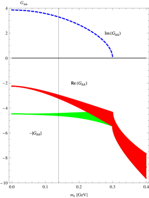
Figure 2: Dependence of the delta axial charge $G_{{\Delta}{\Delta}}$ on the pion mass. The plotted bands account for uncertainty arising from the unknown NLO coupling.

Partially Quenched Chiral Computations.— The partially quenched generalization of the Lagrangian in Eq. (6) reads Sharpe and Shoresh (2001)

$${\mathcal{L}}=\frac{f^{2}}{8}\text{str}\Big{(}\partial^{\mu}\Sigma^{\dagger}\partial_{\mu}\Sigma\Big{)}+\frac{\lambda f^{2}}{4}\text{str}\Big{[}m_{Q}(\Sigma^{\dagger}+\Sigma)\Big{]}-\mu_{0}^{2}\Phi_{0}^{2},$$

where the mass matrix has been generalized to

$$m_{Q}=\text{diag}(m,m,m_{j},m_{j},m,m),$$ (10)

in the isospin limit of the valence and sea sectors. The valence pion mass $m_{\pi}$ is given by $m_{\pi}^{2}=2\lambda m$, while the sea pion mass $m_{jj}^{2}=2\lambda m_{j}$. Finally the valence-sea pion mass $m_{ju}^{2}$ is given by the average of the two. The flavor singlet field $\Phi_{0}$ appearing in Eq. (Chiral Corrections and the Axial Charge of the Delta) is $\Phi_{0}=\text{str}\Sigma/\sqrt{2}$ and has been retained as a device. The axial anomaly allows the singlet mass parameter $\mu_{0}$ to be on the order of the chiral symmetry breaking scale. Subsequently integrating out the singlet yields the correct interactions in the flavor neutral sector of the theory. These are described by the so-called hairpin vertex, see Sharpe and Shoresh (2001).

Baryons fields are described in terms of the $\bf{70}$-dimensional super-multiplet ${\mathcal{B}}_{ijk}$ containing spin-$1/2$ baryons, and the $\bf{44}$-dimensional supermultiplet ${\mathcal{T}}^{\mu}_{ijk}$ containing the spin-$3/2$ baryons. For the embedding of the familiar nucleons and delta into these supermultiplets, as well as their free and interaction Lagrangian, see Labrenz and Sharpe (1996); Savage (2002); Chen and Savage (2002); Beane and Savage (2002). At leading order, the PQ$\chi$PT delta axial current is given by Beane and Savage (2002)

$$J_{\mu 5}^{a} = 2{\cal H}\Big{(}\overline{\cal T}^{\nu}S_{\mu}{\overline{\tau}{}^{a}_{\xi+}}{\cal T}_{\nu}\Big{)},$$ (11)

where $\overline{\tau}{}^{a}_{\xi+}={1\over 2}(\xi\overline{\tau}{}^{a}\xi^{\dagger}+\xi^{\dagger}\overline{\tau}{}^{a}\xi)$, and ${\overline{\tau}}^{a}$ are partially quenched extensions of the isospin generators. Because the axial charge $G_{{\Delta}{\Delta}}$ can be determined from connected quark contractions, Eq. (2), we follow Tiburzi (2005b) and choose the upper $2\times 2$ block of $\overline{\tau}^{a}$ to be the ordinary isospin generators and zeros elsewhere. The constant ${\mathcal{H}}$ can be determined from matching, i.e. ${\mathcal{H}}=g_{{\Delta}{\Delta}}$.

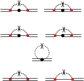
Figure 3: Additional one-loop diagrams contributing to the delta axial charge in PQ$\chi$PT. The cross on the loop meson is a hairpin contribution.

Since we work to next-to-leading order (NLO) in the chiral expansion, we further require contributions from the NLO axial current. These involve one insertion of the quark mass matrix $m_{Q}$

$${\delta}J_{\mu 5}^{a} = \frac{16\lambda}{f^{2}}\Bigg{[}t_{1}{\overline{\cal T}}^{kji}_{\mu}\{\overline{\tau}^{a}_{\xi+}\,,\,{\cal M}_{+}\}^{n}_{i}\ S_{\mu}{\cal T}_{njk}^{\mu}+t_{2}(-)^{\eta_{l}(\eta_{j}+\eta_{n})}{\overline{\cal T}}^{kji}_{\mu}(\overline{\tau}^{a}_{\xi+})^{l}_{i}({\cal M}_{+})^{n}_{j}S_{\mu}{\cal T}_{lnk}^{\mu}$$ (12)

$$+ t_{3}{\overline{\cal T}}^{kji}_{\mu}(\overline{\tau}^{a}_{\xi+})^{l}_{i}S_{\mu}{\cal T}_{ljk}^{\mu}\ {\rm str}({\cal M}_{+})+t_{4}{\overline{\cal T}}^{kji}_{\mu}S_{\mu}{\cal T}_{ijk}^{\mu}\ {\rm str}(\overline{\tau}^{a}_{\xi+}{\cal M}_{+})\Bigg{]}\,,$$

where the mass operator ${\mathcal{M}}_{+}$ is defined by: ${\mathcal{M}}_{+}=\frac{1}{2}\left(\xi^{\dagger}m_{Q}\xi^{\dagger}+\xi m_{Q}\xi\right)$. When working to tree-level, there are only two independent contributions from the NLO current: one is proportional to the valence pion mass squared and the other is proportional to the sea pion mass squared. Compared to $SU(2)$ $\chi$PT there is thus one additional parameter to be determined. At NLO, there are additionally non-analytic contributions arising from the loop diagrams in Figs. 1 and 3. Evaluating these contributions, we find the partially quenched delta axial charge

$$G_{\Delta\Delta} = g_{\Delta\Delta}Z_{\Delta}-\frac{1}{(4\pi f)^{2}}\Bigg{\{}2g_{\Delta\Delta}{\cal L}(m_{ju},\mu)+\frac{11}{9}g^{3}_{\Delta\Delta}\Bigg{[}\frac{2}{3}{\cal L}(m_{\pi},\mu)+\frac{4}{9}{\cal L}(m_{ju},\mu)+{\cal R}(\eta_{u},\eta_{u},\mu)\Bigg{]}$$ (13)

$$+ g^{2}_{\Delta N}\Bigg{[}\frac{8}{9}g_{\Delta\Delta}{\cal K}(m_{ju},-\Delta,\mu)+(g_{A}+g_{1}){\cal J}(m_{\pi},-\Delta,\mu)-(2g_{A}+g_{1}){\cal J}(m_{ju},-\Delta,\mu)\Bigg{]}\Bigg{\}}+{\mathcal{A}}m^{2}_{\pi}+{\mathcal{B}}m_{jj}^{2}.\quad$$

The partially quenched wavefunction renormalization $Z_{\Delta}$ appears in Tiburzi and Walker-Loud (2005), and the function $\mathcal{R}(\phi,\phi^{\prime},\mu)$ which arises from hairpins is given in Jiang and Tiburzi (2008). The constants ${\mathcal{A}}$ and ${\mathcal{B}}$ are shorthands for linear combinations of coefficients from the NLO partially quenched delta axial current, Eq. (12). With Eq. (13), one can extrapolate $G_{{\Delta}{\Delta}}$ in both valence and sea quark masses. Finally with trivial modifications, the mixed action extrapolation can be performed.