Measurement of the Current-Phase Relation in Josephson Junctions Rhombi Chains

Abstract

We present low temperature transport measurements in one dimensional Josephson junctions rhombi chains. We have measured the current phase relation of a chain of 8 rhombi. The junctions are either in the classical phase regime with the Josephson energy much larger than the charging energy, $E_{J}\gg E_{C}$, or in the quantum phase regime where $E_{J}/E_{C}\approx 2$. In the strong Josephson coupling regime ($E_{J}\gg E_{C}\gg k_{B}T$) we observe a sawtooth-like supercurrent as a function of the phase difference over the chain. The period of the supercurrent oscillations changes abruptly from one flux quantum $\Phi_{0}$ to half the flux quantum $\Phi_{0}/2$ as the rhombi are tuned in the vicinity of full frustration. The main observed features can be understood from the complex energy ground state of the chain. For $E_{J}/E_{C}\approx 2$ we do observe a dramatic suppression and rounding of the switching current dependence which we found to be consistent with the model developed by Matveev et al.(Phys. Rev. Lett. 89, 096802(2002)) for long Josephson junctions chains.
PAS number(s): 74.40+k, 74.50+r, 74.81.Fa, 73.23b

I Introduction

Arrays of small Josephson junctions exhibit a variety of quantum states controlled by lattice geometry and magnetic frustration Fazio_2001 . A particularly interesting situation occurs in systems with highly degenerate classical ground states where non trivial quantum states have been proposed in the search for topologically protected qubit statesIoffe_2002 . The building block for such a system is a rhombus with 4 Josephson junctions and the simplest system is the linear chain of rhombi as proposed by Douçot and VidalDoucot_02 along the line of the so-called Aharonov-Bohm cages Vidal_98 . The main consequence of the Aharonov-Bohm cages in the rhombi array is the destruction of the (2e)-supercurrent when the transverse magnetic flux through one rhombus is exactly half a superconducting flux quantum. This destructive interference is reminiscent of the localization effect predicted for non interacting charges in Vidal_98 and considered experimentally in both superconducting networks Abilio_99 and quantum wires Naud_01 . Interestingly, a finite supercurrent carried by correlated pairs of Cooper pairs (carrying a charge of 4e) was predicted to subsist in the case of Josephson junctions with small capacitancesDoucot_02 .

In experimentally relevant situations, the junctions’ capacitances are larger than the ground capacitances of the islands between the junctions. The supercurrent flowing in a linear chain was predicted to be dramatically suppressed, even in chains of rather strong Josephson junctionsMatveev_02 , because of the large probability of quantum phase slip events along the chain. As a result, it is expected that the supercurrent through a phase-biased rhombi chain should be exponentially small.

I. Protopopov and M. FeigelmanProtopopov_04 ; Protopopov_06 have studied the equilibrium supercurrent in frustrated rhombi chains. They have made quantitative predictions for the magnitude of both, the 2e and the 4e supercurrents, as a function of the relevant practical parameters : magnetic flux, ratio of Josephson to Coulomb energy, chain length and quenched disorder. Recently S. Gladchenko et al. reported on the first observation of the coherent transport of pairs of Cooper pairs in a small size rhombi array in the quantum regimeGershenson .

Whether the chain is in the classical or in the quantum regime is set by the ratio between the Josephson energy $E_{J}=i_{c}\frac{\hbar}{2e}$ and the charging energy $E_{C}=\frac{e^{2}}{2C}$ of the junctions. In this paper we present measurements of the current phase relation for long Josephson junctions rhombi chains ($N=8$ rhombi), carried out either in the classical phase regime with the Josephson energy much larger than the charge energy, $E_{J}\gg E_{C}$, or in the quantum phase regime where $E_{J}/E_{C}\approx 2$. In order to measure the current phase relation, we shunted the rhombi chain with a high critical current Josephson junction and measured its switching current as a function of the magnetic flux for different rhombus frustrations.

In chapter II we present the theory describing the states and the energy bands for a rhombi chain in the classical limit. This theory is used later in chapter V in order to understand the measurements of the current-phase relation in classical chains. In chapter III we begin by a general overview of the phenomena occuring in the presence of charging effects. Secondly we present a theoretical description of quantum fluctuations based on a tight binding hamiltonian for the non frustrated regime. Chapter IV presents the sample fabrication and characterization. Chapter V is devoted to the current phase relation measurements in the classical regime where $E_{J}/E_{C}\approx 20$. These results can be understood from the shape of the lowest energy band, whose periodicity changes, as expected, from $h/2e$ at small frustration to $h/4e$ near full frustration. The corresponding measurements in the quantum limit for $E_{J}/E_{C}\approx 2$ as well as a detailed quantitative comparison to the theory are presented in chapter VI. Finally, in the appendix, we analyze the current voltage characteristics of open chains where the total phase is not constrained.

II Classical Energy states of rhombi chains

We are interested in the current phase relation $I_{S}(\gamma)$ of a rhombi chain for different rhombus frustrations $f=\Phi_{r}/\Phi_{0}$. $\Phi_{r}$ represents the magnetic flux inside one rhombus and $\Phi_{0}=\frac{h}{2e}$ is the superconducting flux quantum. The phase difference $\gamma$ over the chain is fixed by introducing the rhombi chain into a superconducting loop threaded by a magnetic flux $\Phi_{c}=\Phi_{0}\gamma/2\pi$. The Josephson junctions circuit and the notations that we will further refer to are represented in Fig.1.

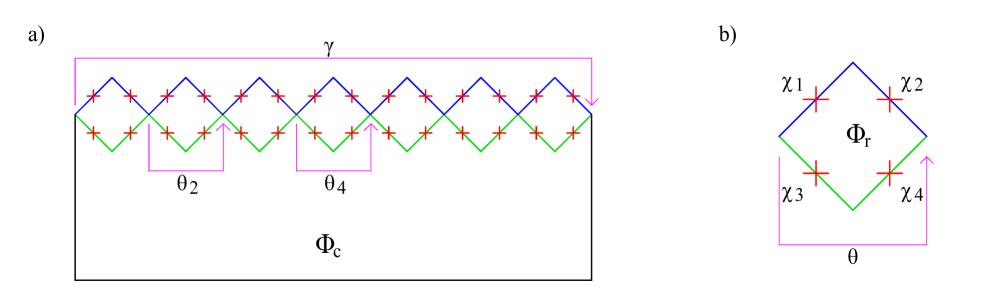
Figure 1: (Color online) The different notations used in the text for the rhombi chain (a) and for one rhombus (b). Each red cross represents a Josephson junction. The lines represent superconducting wires and the arrows represent gage invariant phase differences. The magnetic flux $\Phi_{c}$ inside the superconducting ring containing the rhombi chain fixes the phase difference across the chain to $\gamma=2\pi\Phi_{c}/\Phi_{0}$. The phase differences over each of the four junctions in one rhombus are denoted by $\chi_{n}$ where $n=1,2,3,4$. The gage-invariant phase $\theta$ will be referred as the diagonal phase difference. $\Phi_{r}$ represents the magnetic flux inside one rhombus and the frustration parameter of the rhombus is given by $f=\Phi_{r}/\Phi_{0}$.

In this chapter we discuss the case where charging effects are negligible, and therefore the superconducting phase is a classical variable. The classical states of one rhombus which depend on the diagonal phase difference $\theta$ and on the frustration $f$ are introduced in section A. In section B we extend the classical description of the energy states to a chain containing N rhombi. In this case the energy band depends again on the frustration $f$ and the phase difference $\gamma$ over the whole chain.

II.1 Single Rhombus

We consider a single rhombus made of 4 identical Josephson junctions (Fig.1b) with Josephson energy $E_{J}$ and critical current $i_{c}=\frac{2e}{\hbar}E_{J}$.

a)

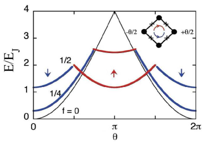
b)

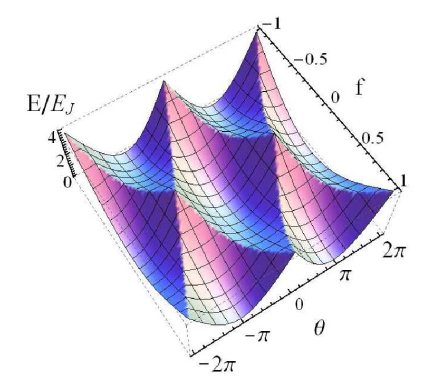
c)

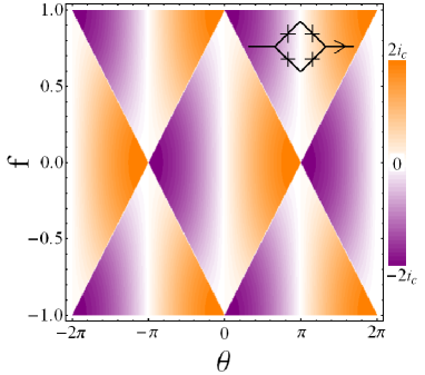
d)

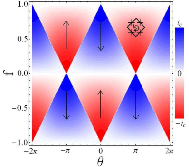
Figure 2: (Color online) Classical states of a single rhombus. a) The ground state energy as a function of the diagonal phase difference $\theta$ over the rhombus for three different frustrations $f=0$, $1/4$ and $1/2$. The inset shows the two possible persistent current states: a clockwise flowing supercurrent (blue lines) and a counterclockwise supercurrent (red line). b) 3D plot showing the lowest energy band as a function of $\theta$ and $f$. c) Two dimensional plot for the supercurrent across one rhombus. The amplitude and sign of the supercurrent is illustrated by the background color: orange(positive values) for currents flowing from left to right and violet(negative values) for currents from right to left. d) Two dimensional plot for the amplitude and the direction of the persistent current around the ring. The clockwise current states, denoted $\left|\downarrow\right\rangle$, are represented in blue, the counterclockwise current states, denoted $\left|\uparrow\right\rangle$, in red. At full frustration ($f=0.5$) the ground state is degenerate for $\theta=\pm\pi/2$, and the two eigenstates differ by the sign of the persistent current.

Neglecting additional terms due to inductances, the potential energy of one rhombus containing four identical junctions, is simply given by the sum of the Josephson energies of the four junctions:

$$E(\chi_{1},\chi_{2},\chi_{3},\chi_{4})=\sum_{n=1}^{4}E_{J}(1-\cos\chi_{n})$$ (1)

The sum of the phases $\chi_{n}$ is fixed by the flux inside the rhombus:

$$\sum\chi_{n}=2\pi f$$ (2)

Using the notations defined earlier, the ground state energy of one rhombus, in the classical regime ($E_{J}\gg E_{C}$), is found by minimizing the energy (1) and depends on the parameters $\theta$ and $f$:

$$E(\theta,f)/E_{J}=4-2(\left|\cos(\theta/2+\pi f/2)\right|+\left|\cos(\theta/2-\pi f/2\right|)$$ (3)

A complete description of the phase diagram for one rhombus is given in Fig.2. The circular current in the superconducting ring is $i_{p}(\theta,f)=\frac{2e}{\hbar}\frac{\partial E(\theta,f)}{\partial f}$ and it is $2\pi$-periodic in $\theta$ and f (Fig.2d). The supercurrent through one rhombus is given by $i_{s}(\theta,f)=\frac{2e}{\hbar}\frac{\partial E(\theta,f)}{\partial\theta}$ and it is shown in Fig.2c.

The interesting feature about this system is the change from $2\pi$ to $\pi$ periodicity as a function of the bias phase $\theta$ over the rhombus when the frustration f changes from $0$ to $1/2$. This property does not exist in the case of a dc SQUID, as there is no modulation of the energy as a function of $\theta$ at full frustration. At $f=1/2$ the rhombus has two classical ground states, $\theta=0,\pi\pmod{2\pi}$, denoted in analogy to the z-projection of the spin $\frac{1}{2}$ by $\left|\downarrow\right\rangle$ and $\left|\uparrow\right\rangle$ respectively. These two states have the same energy $E(\theta=0,f=0.5)=E(\theta=\pi,f=0.5)=2(2-\sqrt{2})E_{J}$ but opposite persistent currents (see Fig.2d). In the case of a current biased rhombus, the phase $\theta$ is controlled via the current phase relation of a single rhombus $i_{s}(\theta,f)=\frac{2e}{\hbar}\frac{\partial E(\theta,f)}{\partial\theta}$ by the external current. The critical current of a single rhombus is given by the maximum supercurrent through the rhombus for a given frustration $f$: $I_{c}=\max(i_{s}(\theta))_{f=const}=\max(\frac{2e}{\hbar}\frac{\partial E(\theta,f)}{\partial\theta})_{f=const}$. It is periodic in $f$ and varies from a maximum of $2i_{c}$ down to $i_{c}$. For $-1/2\leq f\leq 1/2$ it reads :

$$I_{c}=2i_{c}\cos^{2}\frac{\pi f}{2}$$ (4)

II.2 Rhombi chain

In order to understand the classical states of the chain we can start our analysis with the case where each rhombus has a well defined diagonal phase difference across it. For a closed chain of $N$ identical rhombi, the sum of all the diagonal phase differences $\theta_{n}$ is fixed by the magnetic flux $\Phi_{c}$ to a total phase difference $\gamma$ over the chain (see Fig.1a).

$$\sum_{n=1}^{N}\theta_{n}=\gamma$$ (5)

In the region where the frustration, $0\leq f\ll 1$, is small we obtain by minimizing the total energy that the diagonal phase differences over each rhombus are identical up to a constant multiple of $2\pi$. The phase difference across the diagonal of the $n$-th rhombus in the state $|m\rangle$ is given by:

$$\theta_{n}=\frac{\gamma-2\pi m}{N}+2\pi m_{n}\ \;,\;m=\sum_{n}m_{n}$$ (6)

where $m$ is the number of vortices inside the superconducting loop that contains the rhombi chain, and $m_{n}$ is an integer corresponding to the number of vortices that crossed the $n$-th rhombus. Therefore the ground energy of the chain is $N$ times the energy of a single rhombus:

$$E(\gamma,f)/E_{J}=N(4-2(\left|\cos((\gamma-2\pi m)/2N+\pi f/2)\right|+\left|\cos((\gamma-2\pi m)/2N-\pi f/2\right|)$$ (7)

At $f=0$ and in the limit $N>>1$ the expression above can be developed around zero. The energies of the low-lying states are given by:

$$E_{m}(\gamma)=\frac{E_{J}}{2N}\left(\gamma-2\pi m\right)^{2}$$ (8)

The ground state energy consists of a series of shifted arcs, with period $2\pi$ as shown in Fig.3a. In analogy to a single rhombus, at small frustration all rhombi of the chain are in the $\left|\downarrow\right\rangle$ state (see Fig.2). The supercurrent through the chain is given by the derivative of the ground state energy with respect to $\gamma$, $I_{S}(\gamma,f)=\frac{2e}{\hbar}\frac{\partial E(\gamma,f)}{\partial\gamma}$. Therefore the current-phase relation of an unfrustrated chain, in the classical regime, is a $2\pi$-periodic sawtooth function as for a single rhombus. But in contrast to a single rhombus the critical current of a chain with large $N$ is approximatively $N$ times smaller than the critical current of a single junction. The value for the critical current of the chain $i_{c}\frac{\pi}{N}$ can be easily calculated from the energy expansion (8).

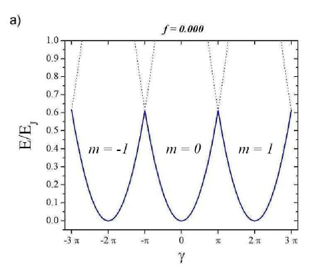
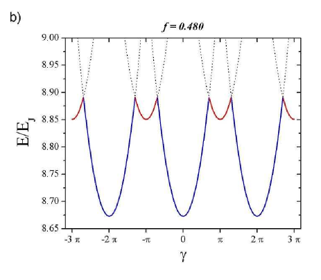
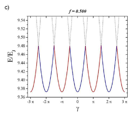
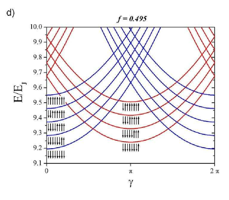
Figure 3: (Color online) a) Ground state energy of a classical 8 rhombi chain as a function of the phase $\gamma$, for zero (a), intermediate (b) and full frustration (c). The plot colors correspond to the $\left|\downarrow\right\rangle$ state (blue) and $\left|\uparrow\right\rangle$ state (red). The supercurrent flowing through the chain is given by the derivative of the energy as a function of $\gamma$ and consists of a series of unequal sawtooth in the vicinity of $f=1/2$. d) Identification of the lowest energy states of the chain near full frustration ($f=0.495$). The up and down arrows indicate the spin states of the $8$ rhombi. Note the change in the parity for the number of switched rhombi between successive minima.

As $f$ approaches $1/2$, the total energy can be reduced by flipping the spin state of one rhombus. The chain with $N-1$ rhombi in the $\left|\downarrow\right\rangle$ state and one rhombus in the $\left|\uparrow\right\rangle$ state becomes energetically more favorable near $\gamma=\pi\pmod{2\pi}$ as shown in Fig.3a. Thus the energy diagram consists of an alternate sequence of arcs, centered respectively at even and odd multiples of $\pi$. At full frustration $f=1/2$, the period as a function of $\gamma$ turns to $\pi$(Fig.3a upper trace). Here, the energy modulation $\frac{\pi^{2}}{8N\sqrt{2}}E_{J}$ and the maximum supercurrent $I_{s}=i_{c}\frac{\pi}{2\sqrt{2}N}$ are significantly weaker than at zero frustration. The crossoverpoint between these two regimes is defined as the minimum frustration that induces at $\gamma=\pi$ a flip from the $\left|\downarrow\right\rangle$ state to the $\left|\uparrow\right\rangle$ state for one single rhombus in the chain. In Fig.3b we represented the state of the system for $f$ slightly larger than the crossover frustration. For large $N$ the width of the frustration window scales with $1/N$ and can be approximated by the condition :

$$1-\tan\frac{\pi f}{2}<\frac{\pi^{2}}{8N}$$ (9)

Within this window, the supercurrent is expected to show a complex sawtooth variation as a function of the phase $\gamma$ with unequal current steps. It is interesting to discuss in more details the structure of the chain states in the vicinity of the full frustration region. In Protopopov_04 it has been shown that near $f=0.5$ the energy of the different possible chain states can be approximated by the formula:

$$E_{m,S^{z}}(\gamma)\approx\frac{E_{J}\sqrt{2}}{4N}(\gamma+N\pi/2+\pi S^{z}-2\pi m)^{2}-\sqrt{2}\delta S^{z}E_{J}+const$$ (10)

where $\delta=2\pi f-\pi$. Here $S^{z}=-\frac{1}{2}\sum$sign$(\sin(\theta_{n}))$ corresponds to the z-projection of the total spin S describing the whole rhombi chain. Figure 3d shows the energy diagram for the lowest energy chain states with N=8 in order to highlight the topological distinctions between branches with minimas at even and odd values of $\gamma/\pi$. Near $\gamma=0$ the ground state is obtained when all the rhombi are in the $\left|\downarrow\right\rangle$ state. Near the next minimum, one rhombus has flipped into the $\left|\uparrow\right\rangle$ state. For the higher energy levels one can conclude in general that at even values of $\gamma/\pi$, chain states containing an even number of rhombi in the $\left|\uparrow\right\rangle$ state (so called even states) show a minimum. At odd values of $\gamma/\pi$ chain states with an odd number of rhombi in the $\left|\uparrow\right\rangle$ state (so called odd states) show a minimum. At full frustration $f=1/2$ all chain states with an even and odd number of flipped rhombi become respectively degenerate. Complete degeneracy is achieved at full frustration at $\gamma=\pi/2$ : even and odd states have the same energy.

In conclusion, the current phase relation of the rhombi chain in the classical regime should follow a sawtooth like function with a slowly varying amplitude as a function of the frustration except for a small region around $f=0.5$. Inside this so called frustration window the periodicity of the sawtooth should double and its amplitude should drop by a factor of $2\sqrt{2}$. In chapter V we present measurements that precisely confirm these predictions.

III Quantum Energy states of rhombi chains

In this chapter we will discuss the influence of charging effects on the current phase relation of the rhombi chain. Section A offers a qualitative overview of the expected phenomena when quantum fluctuations are not negligible. Section B is devoted to a quantitative analysis in the region $f=0$. We develop a tight binding model proposed initially by Matveev et alMatveev_02 for a Josephson junctions chain. This theoretical model will successfully fit our measurements presented in section VI.

III.1 Quantum phase slips

Quantum fluctuations start to play a role when the charging energy $E_{C}$ cannot be neglected anymore in comparison to the Josephson energy $E_{J}$. Quantum fluctuations induce quantum phase slips. For quantum junctions at very low temperature the role of quantum phase slips is twofold. First, phase slip events, even rare, allow the system to tunnel through the energy barriers which separate the local minimums and to reach the ground states discussed above. On the other hand phase slips induce quantum coupling between different states and lead to the formation of macroscopic quantum states extended over the whole chainDoucot_02 ; Matveev_02 ; Protopopov_04 . This superposition of states lifts the high degeneracy of the classical states. In the case of important quantum fluctuations, the crossing points between different states shown in Fig.3 become anticrossing points, strongly modifying the physical properties of the system (see Fig.4). The rate of phase slips depends on the height and shape of the energy barrier which is set by the ratio $E_{J}/E_{C}$. We choose to focus our attention on two extreme cases: $E_{J}\gg E_{C}$ (classical regime) where there are practically no phase fluctuations and $E_{J}/E_{C}\approx 2$ (quantum regime) where the quantum fluctuations open a significant gap between the classical states at the crossing points.

The frustrated and non frustrated regime involve different kinds of tunnelling process:

At $f=0$ (see Fig. 3a) or when $f$ is outside the window defined by equation 9, the energy states cross each other at $\gamma=\pi$ (modulo $2\pi$). The necessary $2\pi$ jump can be achieved by simultaneous phase slips events in two junctions of one rhombus (one junction in each branch). At $f=0$, the simplest path corresponds to a sinusoidal energy barrier of $4E_{J}$ as shown in Fig.5. The rhombi chain can be treated like a Josephson junctions chain considered by Matveev et al. Matveev_02 , except that, here, the tunnel amplitude for quantum phase slips ($v$) involves the simultaneous phase slip on two junctions. We have calculated this tunnel amplitude in the case of a rhombus and the next section presents a detailed description of the tight binding model that we used to fit our experimental results in the quantum regime at $f=0$.

Qualitatively, when quantum fluctuations are large enough, one expects a rounding of the sawtooth-like $2e$ supercurrent turning eventually to a sinusoidal current of exponentially small amplitude, as predicted in Matveev_02 . At finite frustration, the tunnel path is flux dependent and involves more complex trajectories in the multidimensional energy landscape. The tunnel amplitude will presumably be increased.

Figure 4: Energy bands of the rhombi chain in the presence of quantum fluctuations. a) Energy bands of an almost classical chain near full frustration ($f=0.495$). In this regime quantum phase slips mix the degenerate classical levels and lead to the appearance of avoided level crossings. b) First two energy bands of the quantum chain at full frustration ($f=0.5$). Deep in the quantum regime fluctuations mix a lot of different classical levels and the spectrum is no longer piecewise parabolic. The precise form of the spectrum can be calculated on the basis of the Eq. (16) of the reference Protopopov_04 . Figure b) was generated by taking $E_{J}/E_{C}=6$.

Near $f=1/2$, the successive energy minima as a function of $\gamma$ have periodicity $\pi$. The corresponding chain states differ by the sign of the persistent current in one rhombus. Here the transition requires a phase jump of $\pi$ across one rhombus. The energy barrier for this process can be approximated by considering a path in the parameter space where a single junction switches by $2\pi$. In this case the energy barrier is close to a sinusoidal barrier with height $2(\sqrt{2}-1)E_{J}$, $i.e.$ $0.414$ times the energy barrier for a single junction.

III.2 Quantum fluctuations of the rhombi chain at zero magnetic field

In the region where the frustration is small, $0\leq f\ll 1$, the theory we develop here is just a slight modification of the analysis carried out in Matveev_02 for a chain of single Josephson junctions. The reason for this similarity is that around zero frustration the energy of a single rhombus as a function of the phase difference across it has only one minimum (see Fig.2a). This implies the coincidence of the classification of the classical states for our system and for the single Josephson junctions chain. In this section we present the theory of quantum fluctuations in a non-frustrated rhombi chain which we used to fit the experimental data. In our analysis we assume that the Josephson energy of the junctions is much larger than the charging energy and quantum fluctuations in individual Josephson junctions are small. However, as we will see below, the fluctuations in the whole chain can be strong.

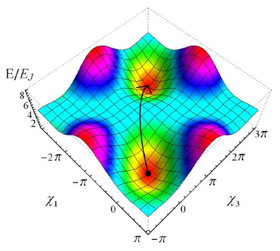
Figure 5: (Color online) The energy landscape for one rhombus at zero frustration ($f=0$) as a function of the phase differences $\chi_{1}$ and $\chi_{3}$ of Josephson junctions in opposite branches of the rhombus. The transition of the chain from state $\left|m\right\rangle$ to state $\left|m+1\right\rangle$ corresponds to a $2\pi$ jump of one of the diagonal rhombus phases $\theta_{n}$. This transition implies a simultaneous flip of the two phases $\chi_{1}$ and $\chi_{3}$ respectively by $-2\pi$ and $2\pi$. The arrow in the figure represents the corresponding classical trajectory. The phenomenon can also be seen as the process of one vortex crossing the rhombus ring.

Quantum fluctuations (more precisely quantum phase slips) lead to the mixing of classical states described above. At large $E_{J}/E_{C}$ this effect can be described within the tight-binding approximation (cf. Matveev_02 ). Classical states lie far from each other in the configuration space and are separated by barriers of the order $E_{J}$ (see Fig.5). At large $E_{J}/E_{C}$ the amplitude of quantum tunnelling from state $\left|m\right\rangle$ to $\left|m^{\prime}\right\rangle$ is exponentially small and decreases fast with the increase of the distance between $\left|m\right\rangle$ and $\left|m^{\prime}\right\rangle$. For a given state $\left|m\right\rangle$ the closest states in the configuration space are $\left|m\pm 1\right\rangle$. To achieve the state $\left|m+1\right\rangle$ one needs to change the phase difference across the diagonal of one rhombus by $2\pi$ (at large $N$, cf. eq. (6)). Since we need to maintain the sum of the phase differences around the rhombus (fixed by the zero flux inside it, see eq. (2)) we need to change by $\pm 2\pi$ the phase differences over two junctions in different branches of the rhombus (see Fig.5). Let us denote the amplitude of such a process by $\upsilon$. In a semiclassical approximation this amplitude is determined by the vicinity of the classical trajectory connecting states $\left|m\right\rangle$ and $\left|m+1\right\rangle$ in imaginary time

$$\upsilon=A\exp\left(-S_{0}\right)$$ (11)

Here $S_{0}$ is the imaginary-time action on the classical trajectory (instanton). As it is easy to see from the preceding discussion, $S_{0}$ is just twice the action describing a phase slip in a single junction. We thus have (cf. equation 7 of the reference Matveev_02 , note the difference in the definitions of $E_{C}$ in this paper and in Matveev_02 )

$$S_{0}=2\sqrt{\frac{8E_{J}}{E_{C}}}$$ (12)

The coefficient $A$ in (11) accounts for the contribution of the trajectories close to the classical one. Standard calculation gives

$$A\approx 4.50(E_{J}^{3}E_{C})^{1/4}$$ (13)

We can now construct the tight-binding Hamiltonian describing the effect of the phase slips on the properties of the chain

$$H|m\rangle=E_{m}|m\rangle+4N\upsilon|m+1\rangle+4N\upsilon|m-1\rangle$$ (14)

The coefficient $4$ in the total tunneling matrix element is due to the number of possible tunneling paths within one rhombus while $N$ appears here because of the fact that a phase slip in any rhombus brings the system to the same state.

Following now the procedure described in Matveev_02 we can reduce the problem of finding the eigenvalues of the Hamiltonian (14) to the solution of the Mathieu equation

$$\psi^{\prime\prime}(x)+(a-2q\cos 2x)\psi(x)=0\,,\qquad\psi(x+\pi)=e^{i\gamma}\psi(x)$$ (15)

The parameters of the Mathieu equation are defined by

$$a=\frac{2NE}{\pi^{2}E_{J}}\,,\qquad q=\frac{8N^{2}\upsilon}{\pi^{2}E_{J}}$$ (16)

Here $E$ is the energy of the rhombi chain.

The equation (15) can be solved analytically in different limiting cases (see ref. Matveev_02 for details). By solving it numerically and using the general relation $I_{S}=\frac{2e}{\hbar}dE/d\gamma$ one can find the current-phase relation for the rhombi chain at arbitrary fluctuations’ strength. This is the exact procedure that we have used in chapter VI in order to fit the measured current-phase relation for quantum chains. We found a very good agreement between the theoretical predictions and the measured data.

IV Sample fabrication and characterization

The samples were made by standard e-beam lithography and shadow evaporation technique using a Raith Elphy Plus e-beam systemRaith and an ultra high vacuum evaporation chamber. They consist of small arrays of $Al/AlO_{x}/Al$ tunnel junctions deposited on oxidized silicon substrates. The respective thicknesses of the Al layers were 20 and 30 nm.The tunnel barrier oxidation was achieved in pure oxygen at pressures around $10^{-3}mbar$ during 3 to 5 minutes depending on the sample. The samples were mounted in a portable closed copper block which was thermally anchored to the cold plate of either a $He^{3}$ insert or a dilution fridge. All lines were heavily filtered by thermocoaxial lines and $\pi-$filters integrated in the low temperature copper block. Additional low frequency noise filters were placed at the top of the cryostat.

Figure 6: Schematic of the circuit designed to measure the current phase relation in a rhombi chain. The chain is closed by a superconducting line interrupted by an additional Josephson junction referred to as the ”shunt junction”. An external magnetic field $B$ allows the control of both the rhombi frustration $f$ and the total phase of the closed chain $\gamma$.

In order to measure the current-phase relation, we introduced the rhombi chain in a closed superconducting loop which contains an additional shunt Josephson junction as shown in Fig.6. We have measured the switching current of this circuit. The switching current was obtained from the switching histogram. We fixed the threshold voltage at about one third of the shunt junction gap voltage. The histograms were accumulated at a rate $10kHz$ using a fast trigger circuittrigger . The bias current was automatically reset to zero immediately after each switching event. The switching current $I_{SW}$ corresponds, in our definition, to an escape probability of $50\%$.

As the critical current of the shunt junction is much larger than the critical current of the chain, near the switching event the phase difference over it is close to $\pi/2$. Therefore the flux $\Phi_{c}$ changes only the phase difference $\gamma$ over the chain. The switching current through the parallel circuit represented in Fig.6 can be written as the sum of the partial supercurrents in the two branches.

$$I_{SW}=I_{S}(\gamma-\frac{\pi}{2})+I_{c}\sin(\frac{\pi}{2})$$ (17)

Here, $I_{S}(\gamma)$ is the supercurrent in the rhombi chain and $I_{c}$ is the shunt junction critical current. Therefore the $\gamma$ dependence of the switching current of the shunted rhombi chain directly reflects the current phase relation of the rhombi chain.

The frustration inside the rhombi chain was controlled by a constant external perpendicular magnetic field. The flux inside the closed chain could be either applied simultaneously or swept independently using control lines. In the first case the two parameters $\gamma$ and $f$ are linked by the area ratio between the rhombus and the ring (see Table 1). Since the rhombus area is much smaller than the ring area, using small variations of the magnetic field $B$ we can vary the phase $\gamma$ for an approximately constant value of $f$.

To be able to achieve reversible fine tuning of the phases, we found it crucial to avoid any flux trapping in the vicinity of the superconducting circuit. For this purpose the superconducting leads were patterned with linear open voids which ensure free motion of vortices. Different sample designs were investigated including open and closed chains. The typical elementary junction area ranged from $0.15\times 0.15\mu m^{2}$ to $0.3\times 0.6\mu m^{2}$. The Josephson energy was inferred from the experimental tunnel resistance of individual junctions and the nominal Coulomb energy was estimated from the junction area using the standard capacitance value of $50fF/\mu m^{2}$ for aluminum junctions. In general, the measured area of the junctions was slightly smaller than expected. The actual Coulomb energy is therefore larger (by about $20\%$) than its nominal value.

We designed, for this experiment, a series of samples as shown in Fig.7. $E_{J}$ and $E_{c}$ as well as the number of rhombi were chosen near the range of the optimum parameters prescribed in Ref Protopopov_04 . The shunt junction has a critical current about $10$ times larger than the switching current of the chain. Fig.7c shows a SEM image of one rhombus. The actual design of the resist mask was optimized to insure the best homogeneity of junction critical currentshomogeneity .

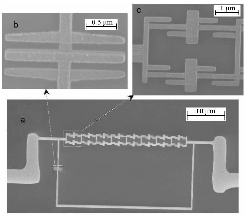
Figure 7: a) SEM image of a rhombi chain ($N=8$, sample C) in the closed superconducting circuit. The shunt junction is visible on the left vertical line. b) An enlarged image of one rhombi is also presented. c) For small magnetic field variations, the flux inside the rhombi practically remains constant, while the total phase on the array varies.

We concentrate on results for three particular samples with the following common characteristic parameters : number of rhombi $N=8$, rhombus area : $2\times 4\mu m^{2}$, shunt junction : $0.15\times 2\mu m^{2}$. Other parameters are listed in Table 1.

Table 1: Characteristic parameters of the samples. For sample A, $E_{J}$ was obtained from the tunnel resistance measured on a reference open chain fabricated on the same chip. For sample B, $r_{n}$ (not measured) was estimated to be similar. The charging energy was inferred from the nominal junction area. $R_{shunt}$ ($\Omega$) is the tunnel resistance of the shunt junction.

sample	ring area	rhombi junctions area	$E_{c}(K)$	$r_{n}(\Omega)$	$E_{J}(K)$	$E_{J}/E_{c}$	$R_{shunt}$
A	$8\times 40\mu m^{2}$	$0.15\times 0.30\mu m^{2}$	0.43	$850$	9.0	$20$	$169$
B	$18\times 36\mu m^{2}$	$0.15\times 0.30\mu m^{2}$	0.43	$-$	$-$	$-$	$167$
C	$18\times 36\mu m^{2}$	$0.15\times 0.15\mu m^{2}$	0.8	$4860$	1.6	$2$	$627$

V Classical chains

The observed dependence of the switching current $I_{SW}$ $vs$ the external magnetic flux is shown in Fig.8. Both the rhombi frustration $f$ and the phase along the main ring $\gamma$ are controled by the magnetic field.

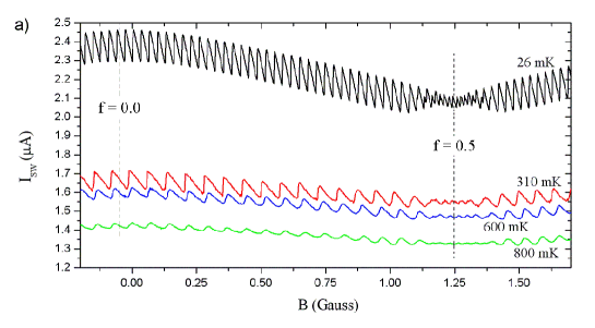
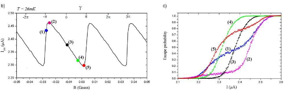
Figure 8: (Color online) a) Experimental plot of the switching current $vs$ external magnetic field at different temperatures. The sample B was measured at the lowest temperature $T=26mK$. The higher temperature measurements correspond to the sample A. b) Magnification of the region near rhombi frustration $f=0$. c) The switching probability of the circuit rhombi chain + shunt junction (sample B) $vs$ current bias at different magnetic fields which correspond to the numbered points indicated in figure 8b.

We observe a complex dependence of $I_{SW}$ as a function of the magnetic flux with mainly one slow periodic envelop of period $2.57$ Gauss that we attribute to the frustration inside the rhombus and one fast sawtooth oscillation that we understand as the modulation of the supercurrent as a function of the phase $\gamma$. The number of periods differs for the two samples A and B as expected from the difference between the ring areas.

We have verified that the fast modulation is periodic with period $h/2e$ except near $f=1/2$ where the period is $h/4e$ (see Fig.8a and Fig.10b). This result confirms precisely what is illustrated in Fig.3 : the chain states undergo a transition from phase periodicity $2\pi$ to periodicity $\pi$ when the rhombi are fully frustrated. Let us notice here that the half periodicity is not actually visible over many periods since the control magnetic flux changes both the frustration and the phase. Instead, we do observe a sequence of saw teeth with unequal amplitudes which become regular only at exactly $f=1/2$. We have confirmed the period halving in a separate experiment where we used on-chip superconducting lines to control $f$ and $\gamma$ separately. We could observe up to 12 oscillations (not shown) of the critical current $vs$ $\gamma$ when the rhombi frustration was fixed exactly at $f=1/2$ by a static magnetic field $B=1.29$ gauss.

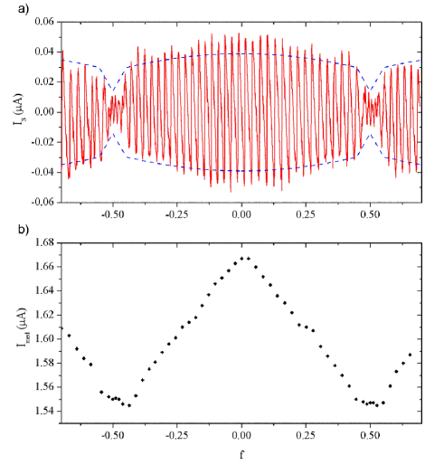
Figure 9: (Color online) The fast oscillation component $I_{s}$ (a) and the median component $I_{med}$ (b) of the switching current in sample A at $T=310mK$. The plot (a) represents the supercurrent through the chain and the plot (b) gives the additional contributions coming from the shunt junction and the rhombi chain (see text). The expected amplitude of the supercurrent is shown as dotted lines in trace (a).

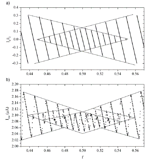
Figure 10: Comparison between the measured switching current of sample B (b) and the theoretical persistent current (a) in the classical limit (see section II) near $f=1/2$. The lines joining the cusps are guides for the eyes. The vertical axis in (a) is in units of the single junction critical current $i_{c}$.

The different histograms shown in Fig.8c illustrate how the switching probability evolves within one fast period of the $I_{SW}$ sawtooth. The sharpest histogram is obtained in the middle of the linear sawtooth $i.e.$ when the supercurrent goes to zero (minimum of energy in the parabolic diagram shown in Fig.3a). For this point the state of the chain is quite stable. The presence of two steps in the histogram near the maximum or minimum of the sawtooth could be an indication that the system can switch between the states $\left|m\right\rangle$ and $\left|m+1\right\rangle$. They reveal the crossing of energy levels between successive parabolic arcs of the energy diagram. The whole plot evolves slightly when the criterion for the definition of the switching current is set different from $50\%$ but the main features are preserved. The observed behaviour at 26mK is characteristic for the zero temperature limit. We saw no change with increasing moderately the temperature. The trace remained very similar except for a small change in the vertical scale. For example at $326$ mK the amplitude of the fast oscillation was found to decrease by about $6\%$ and $10\%$ for the $h/2e$ and the $h/4e$ components respectively. We also observed very rare flux jumps which manifest themselves as discontinuities in the $I_{SW}$ $vs$ $\gamma$ curve. Further reduction of the oscillation amplitude was observed at higher temperature (up to $0.8K$) together with some thermal smearing.

Practically we analyze the $\gamma-$dependence of the switching current as the sum of 3 distinct contributions : a constant level that can be assigned to the switching current of the shunt junction, a fast oscillation due to the persistent current in the large superconducting loop containing the large junction and an additional contribution reminiscent of the switching current of the open chain. In Fig.9a, we have extracted the fast oscillating component $I_{s}$ of the measured switching current of sample A from the median line $I_{med}$ obtained by joining the middle points of each branch of the sawtooth in Fig.8a. The median line (Fig.9b) is reminiscent of the switching current of the reference open rhombi chain which was measured separately (Fig.14). The exact cause for this resemblance is not yet understood. From the measurements we estimate the switching current of the shunt junction at $1.43\mu A$, which looks reasonable.

The fast oscillating component is shown in Fig.9a. The main features of this experimental result follow the theoretical predictions summarized in Fig.3. Since by changing the magnetic field we vary in the same time the frustration and the phase, we obtain supercurrent oscillations with a modulated amplitude. In Fig.9a we have also plotted the theoretical envelop $I_{env}$ (dotted lines) of the supercurrent as calculated for the actual junction parameters in the classical limit. This line is given by the maximum of the supercurrent $I_{S}(\gamma)$ and except for the two small windows visible near $f=\pm 1/2$ it is given by $I_{env}=i_{c}\frac{\pi}{N}\cos(f/2)$ (here $N=8$). Within the frustration window (see eq. (9) and Fig.10), $I_{env}$ falls linearly to its minimum value $i_{c}\frac{\pi}{2\sqrt{2}N}$ at $f=\pm 1/2$, as theoretically expected.

As it can be seen, the measured amplitude of the supercurrent coincides fairly well with the classical value obtained from the nominal critical current of the individual junctions. It appears that the rate of quantum phase slip is too slow to achieve the quantum superposition of classical states and form the macroscopic $4e$ condensate. This is not surprising considering that the ratio $E_{J}/E_{c}=20$ is significantly larger than the optimum values calculated in Protopopov_04 . No rounding or exponential weakening of the sawtooth-like supercurrent is observed. Rather we do see the signature of the succession of classical states forming the ground state illustrated in Fig. 3. The same is true for sample B.

The detailed field dependence of the fast oscillation contribution can be very well understood from the classical ground state of the phase biased rhombi chain. Fig.10 displays the experimental switching current $I_{SW}$ together with the calculated supercurrent near $f=1/2$ for sample B. This sample has the largest ring area and therefore the largest number of fast oscillations. We observe the emergence of the half period in a frustration window $0.447<f<0.553$ as expected from eq. (9) for $N=8$ rhombi. Some additional secondary cusps, presumably due to flux jumps are also observed in the experimental trace.

VI Quantum chains

In order to characterize the regime of quantum fluctuations, experiments on rhombi chains with a ratio of $E_{J}/E_{C}\approx 2$ were performed. The measured histograms, unlike in the case of the classical chains, do not split into steps. Such a behavior is expected in the case where a significantly large gap opens in between the classical states at the cross over point, and thus it prevents the excitation of the system. In our case however, the width of the histograms of $\approx 45nA$ is much larger than the amplitude of the switching current oscillations (see Fig.11). So even if there were some transitions twards the first excited state (measurement induced or thermal excitations, noise), the splitting of the histograms would not be visible.

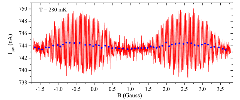
Figure 11: (Color online) In red: the experimental plot of the switching current $vs$ external magnetic field for the sample C at the temperature $T=280mK$. Blue points: the median component of the switching current.

Fig.11 shows the dependence of the measured switching current as a function of the applied magnetic field. As in the case of the classical chain, the signal can be seen as a superposition of three components. The modulated oscillating component characterizes the dependence of the supercurrent of the chain as a function of both the frustration and the phase difference $\gamma$. The oscillations are periodic with period $h/2e$. As we approach the frustrated regime no oscillations of the supercurrent are measured: in the region $f=1/2$ the supercurrent of the chain is strongly suppressed and smaller than the $\approx 1nA$ noise of our experiment.

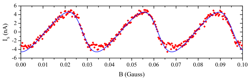
Figure 12: (Color online) The experimental plot (red points) of the switching current $vs$ external magnetic field in the zero frustration region for the sample C at $T=280mK$. The line (in blue) represents the theoretical fit which gives an effective value for the Josephson energy $E^{*}_{J}=0.5E_{J}$.

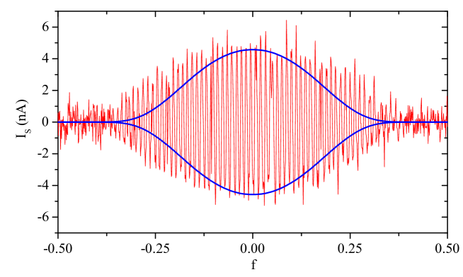
Figure 13: (Color online) In red: the measured switching current oscillations as a function of the frustration $f$. The blue line gives the theoretical prediction for the amplitude of the switching current oscillations by using an effective value $E^{*}_{J}=0.5E_{J}$.

The median component $I_{med}$, shown in Fig.11, as in the case of the classical chains, shows a periodic evolution as a function of the frustration. We measure an amplitude of about $1nA$ for the $I_{med}$ oscillations. The exact cause of this periodic behavior for chains where the phase difference is fixed, was not yet understood. We did a detailed quantitative analysis of the current phase relation at zero flux frustration. Fig.12 shows the measured current phase relation in the non frustrated regime that can be perfectly fitted by the theory described in section III, part B. The only fitting parameter is the Josephson energy $E^{*}_{J}$ for which we find half of the experimental determined one. We can imagine two possible sources for this discrepancy. Firstly the experimental value for $E^{*}_{J}$ has been deduced from the normal state resistance measurement of the large Josephson junction (that is in parallel to the rhombi chain) by supposing the ratio between the two resistances to be the same than the one between the junction areas. This assumption is not always valid in the case that oxidation can occur differently for small junctions than for larger ones. The second source of discrepancy could originate in applicability of the theory described in section III. Formally the description presented above relies on the assumption $E_{J}\gg E_{C}$. On the other hand, even for $E_{J}\sim E_{C}$ the matrix $\upsilon$ for the single tunneling event is much smaller than $E_{J}$. This means that we still can describe the system with the tight-binding Hamiltonian (14) but the precise value of $\upsilon$ can deviate from the one given by equations (11, 12, 13).

To the best of our knowledge this result constitutes the first experimental confirmation of the model proposed by Matveev et al. Matveev_02 for the current-phase relation in long Josephson junction chains.

As we increase the applied magnetic field, the frustration inside the rhombi modifies the value of the effective Josephson energy, which becomes $E_{J}cos(\pi f)$. Using this value, we calculated the evolution of the critical current as a function of the frustration $f$. Fig.13 presents both the results of the calculations and the measured values for the critical current. We can see that the model gives a quantitative description for the measured current amplitude dependence in the non frustrated regime while it can only give a qualitative description in the frustrated region.

VII Conclusion

In this paper we have studied the properties of one-dimensional Josephson junction chains where the elementary cell is a rhombus made of 4 small tunnel junctions. In the classical phase regime, the current-phase relation shows the characteristic sawtooth-like variation. Its periodicity corresponds to the ordinary superconducting flux quantum $h/2e$ when the rhombi chain is non frustrated and it turns to half the flux quantum $h/4e$ at maximum frustration. For large $E_{J}/E_{C}$ ratio the observed current-phase relation can be well understood from the classical ground state of the chain. The latter consists of a sequence of successive parabolas differing by the entrance of phase slips into the chain. Experiments on rhombi chains in the quantum regime ($E_{J}/E_{C}\approx 2$) show a significant reduction and rounding of the current-phase relation in the non frustrated region and a complete suppression of the supercurrent at maximal frustration. In the non frustrated regime we were able to apply for the first time the model proposed by Matveev et al.Matveev_02 in order to successfully fit the measured current phase-relation for an eight rhombi quantum chain.

VIII Acknowledgment

The authors are grateful to B. Douçot, M. Feigelman and L. B. Ioffe for many inspiring discussions. We are indebted to Th. Crozes for his help in sample design and fabrication. The samples were realized in the Nanofab-CNRS platform. We also acknowledge the INTAS program ”Quantum coherence in superconducting nanocircuits”, Ref. 05-100008-7923 for financial support.

IX Appendix : characterization of open chains

In this appendix we consider the transport properties of current biased Josephson chains connected to external reservoirs. Since the chains are open, the phase condition given in eq. (5) does not hold. In this configuration, the switching current of the circuit $I_{SW}$ coresponds to the maximum supercurrent through the chain and it strongly depends on the frustration. We have measured the current-voltage characteristics of chains based on three different elementary cells: a single junction, a SQUID or a rhombus, with lengths varying from $N=1$ to $N=64$. The range of junction parameters is the same as in the main part of this paper. Our general observations are the following :

The current voltage characteristic of chains with large Josephson coupling energy ($E_{J}/E_{C}\gg 10$) is similar to that of a single cell with a multiplicative factor $N$ in voltage. The I-V characteristics are strongly hysteretic and, for small $N$, the switching current is close to the Ambegaokar-Baratoff value. In rhombi chains, the switching current is periodic with respect to the frustration, in particular it drops by a factor 2 at frustration $1/2$ as expected from eq. (4). The SQUID chain exhibits the usual sinusoidal dependence with full cancellation of switching current at frustration $1/2$. It behaves as a chain of single junctions which Josephson energy is tuned by the external magnetic flux. The observation of a fully developed critical current indicates that the chains can be seen as a series of independent cells which remain in a metastable state of energy much higher than the ground state energy shown in Fig.3a for the closed chain. This fact is not surprising since the energy barrier for phase jumps is very high in these strong chains.

Increasing the length or decreasing the Josephson coupling results in a dramatic reduction of the switching current. For example Fig.14 shows the switching current measured in a rhombi chain with $N=8$, made with identical fabrication parameters and on the same chip as sample A (see Table 1). The zero field switching current is about $1/3$ of the Ambegaokar-Baratoff value although the ratio $E_{J}/E_{C}$ is large. The I-V characteristic for this class of samples is hysteretic except near full frustration.

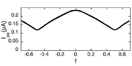
Figure 14: Switching current of a $N=8$ open rhombi chain $vs$ frustration. The $E_{J}/E_{C}$ ratio is 27 and the Ambegaokar-Baratoff critical current is $0.74\mu A$.

A distinct behavior is found in weaker junctions ($E_{J}/E_{C}\leq 10$), when the rate of thermal and quantum phase slips is significant at the time scale of an experiment. On the same chip we fabricated a set of chains where the elementary cell is formed by a single Josephson junction of area $0.15\times 0.3\mu m^{2}$. The chains contained respectively 1, 4, 16 and 64 jonctions. The tunnel resistances per individual junction were found almost identical $r_{n}=3\pm 0.2k\Omega$ which is an indication of good homogeneity of the array. We observed step-like characteristics with voltage jumps equal to the superconducting gap $2\Delta$. Each jump corresponds to the switching of one junction, see Fig.15. We identify the switching current $I_{SW}$ at the first jump, $i.e.$ when the weakest junction runs into a voltage state. For $N=16$, $I_{SW}$ is about 10 times smaller than the expected single junction critical current.

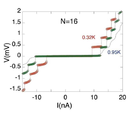
Figure 15: (Color online) Current voltage characteristics of a weak coupling N=16 Josephson chain at temperatures $T=0.32$, $0.8$, and $0.95K$. The elementary voltage jump coresponds to twice the value of the superconducting gap $\Delta=200\mu eV$. The ratio $E_{J}/E_{C}\approx 6$ and the Ambegaokar-Baratoff critical current of a single junction $i_{c}\approx 100nA$.

We found the following characteristics as a function of the chain length :
- The switching current reduces as the chain length $N$ increases : $23,10$ and $1.2$ nA respectively for $N=4,16$ and $64$. We also observe that $I_{SW}$ increases with increasing temperature, indicating that the thermal fluctuations restore the phase coherence of the chain by suppressing quantum processes.
- The hysteresis of I-V curves is suppressed in long chains, giving rise to a regular staircase shape.
- The Josephson branch becomes more and more dissipative as the chain length increases. The measured zero bias resistances are respectively $40$, $380$ and $50k\Omega$ for $N=4$, $16$ and $64$. Further reduction of $E_{J}$ leads to the total suppression of the Josephson coupling in the chain.
The very regular sequence of steps cannot be due to sample inhomogeneities. We believe that the local environment of the different junctions inside the chain plays a significant role. Preliminary experiments where a Josephson chain was shunted by a on-chip interdigit capacitance ($1pF$) did not reveal any significant change.
Up to now we have no quantitative understanding of these observations on open chains.

References

- (1) K.A. Matveev, A.I. Larkin and L. I. Glazman, Phys. Rev. Lett. 89, 096802(2002).
- (2) R. Fazio and H. S.J. van der Zant, Phys. Rep. 355 235 (2001).
- (3) L. B. Ioffe and M. V. Feigel man, Phys. Rev. B66, 224503 (2002).
- (4) B. Douçot and J. Vidal, Phys. Rev. Lett. 88, 227005 (2002).
- (5) J. Vidal, R. Mosseri and B. Douçot Phys. Rev. Lett. 81, 5888 (1998).
- (6) C. C. Abilio, P. Butaud, Th. Fournier, B. Pannetier, J. Vidal, S. Tedesco, and B. Dalzotto, Phys. Rev. Lett. 83, 5102 (1999).
- (7) C. Naud, G. Faini, and D. Mailly, Phys. Rev. Lett. 86, 5104, (2001).
- (8) I. Protopopov and M. Feigel’man, Phys. Rev. B70, 184519 (2004).
- (9) I. Protopopov and M. Feigel’man, Phys. Rev. B74, 064516 (2006).
- (10) S. Gladchenko, D. Olaya, E. Dupont-Ferrier, B. Doucot, L. B. Ioffe and M. E. Gershenson, Cond. Mat. 0802.2295 (2008)
- (11) is the magnetic field times the average area defined by the internal and external contours of the rhombi chain. To be specific, our phase coincides with the term defined in RefProtopopov_04 .
- (12) Raith GmbH, Dortmund, Germany, http://www.raith.de/
- (13) V. Ambegoakar and A. Baratoff, Phys. Rev. Lett. 10, 486 (1963).
- (14) We noticed in our previous designs a few difference in the area of neighbour junctions leading to a small systematic inhomogeneity of critical currents. Here we made a new design which insures that any possible drift of the e-beam induced identical deformation on the shape of each junction. Dispersion of junctions sizes was finally not detectable.
- (15) F. Balestro, J. Claudon, J.P. Pekola and O. Buisson, Phys. Rev. Lett. bf 91, 158301 (2003), for details see F. Balestro, PhD thesis (University J. Fourier 2003), http://tel.archives-ouvertes.fr/tel-00004224/fr/