Spectral fluctuations of billiards with mixed dynamics: from time series to superstatistics

Abstract

A statistical analysis of the eigenfrequencies of two sets of superconducting microwave billiards, one with mushroom-like shape and the other from the familiy of the Limaçon billiards, is presented. These billiards have mixed regular-chaotic dynamics but different structures in their classical phase spaces. The spectrum of each billiard is represented as a time series where the level order plays the role of time. Two most important findings follow from the time-series analysis. First, the spectra can be characterized by two distinct relaxation lengths. This is a prerequisite for the validity of the superstatistical approach which is based on the folding of two distribution functions. Second, the shape of the resulting probability density function of the so-called superstatistical parameter is reasonably approximated by an inverse $\chi^{2}$ distribution. This distribution is used to compute nearest-neighbor spacing distributions and compare them with those of the resonance frequencies of billiards with mixed dynamics within the framework of superstatistics. The obtained spacing distribution is found to present a good description of the experimental ones and is of the same or even better quality as a number of other spacing distributions, including the one from Berry and Robnik. However, in contrast to other approaches towards a theoretical description of spectral properties of systems with mixed dynamics, superstatistics also provides a description of properties of the eigenfunctions. Indeed, the inverse $\chi^{2}$ parameter distribution is found suitable for the analysis of experimental resonance strengths in the Limaçon billiards within the framework of superstatistics.

I Introduction

Integrable Hamiltonian dynamics is characterized by the existence of as many conserved quantities as degrees of freedom. Each trajectory evolves on an invariant hyper-torus in the phase space lichtenberg ; chandre . In contrast, chaotic systems are ergodic; almost all orbits fill the energy shell in a uniform way. Physical systems with integrable and fully chaotic dynamics, respectively, are, however, exceptional. A typical Hamiltonian system shows a phase space in which regions of regular motion and chaotic dynamics coexist. These systems are known as mixed systems. Their dynamical behavior is by no means universal, as is the case for fully regular and fully chaotic systems. If we perturb an integrable system, most of the periodic orbits on tori with rational frequencies disappear. However, some of these orbits persist. Elliptic periodic orbits appear surrounded by islands. They correspond to librational motions around these periodic orbits and reflect their stability. The Kolmogorov-Arnold-Moser (KAM) theorem states that invariant tori with a sufficiently incommensurate frequency vector are stable with respect to small perturbations. Numerical simulations show that when the perturbation increases more and more tori are destroyed. For large enough perturbations, there are locally no tori in the considered region of phase space. The break-up of invariant tori leads to a loss of stability of the system, that is, to chaos. There are three main scenaria of transition to global chaos in finite-dimensional (nonextended) dynamical systems, one via a cascade of period-doubling bifurcations, a Lorenz system-like transition via Hopf and Shil’nikov bifurcations, and the transition to chaos via intermittency eckmann ; bunimovich . It is natural to expect that there are other (presumably many more) such scenaria in extended (infinite-dimensional) dynamical systems.

In quantum mechanics, the specification of a wave function is always related to a certain basis. In integrable systems the eigenbasis of the Hamiltonian is known in principle. In this basis, each eigenfunction has just one component. That obviously indicates the absence of complexity. In the nearly ordered regime, mixing of quantum states belonging to adjacent levels can be ignored and the energy levels are uncorrelated. The level-spacing distribution is well described by that for random numbers generated by a Poissonian process, $\exp(-s)$, where $s$ is the spacing between adjacent energy levels rescaled to unit mean spacing $D$. For a Hamiltonian with a chaotic classical limit, on the other hand the wavefunction components are on average uniformly distributed over the whole basis. Berry berry conjectured that the wavefunctions of chaotic quantum systems can be represented as a formal sum over elementary solutions of the Laplace equation in which the real and imaginary parts of the coefficients are independent identically-distributed Gaussian random variables with zero mean and variance computed from the normalization. Bohigas et al. bohigas put forward a conjecture (strongly supported by accumulated numerical and experimental evidence and also by recent advances towards a proof of this conjecture haakestuff ) that the spectral statistics of chaotic systems follow random-matrix theory (RMT, see mehta ; guhr ). The properties of a chaotic Hamilton operator can thus be modeled by an ensemble of random Hermitian matrices $H$ that belongs to one of three universality classes, either the orthogonal, the unitary or the symplectic one and is called Gaussian orthogonal (GOE), unitary (GUE) and symplectic (GSE) ensemble, respectively. The theory is based on two main assumptions: the matrix elements are independent identically-distributed random variables and their distribution is invariant under unitary transformations. This leads to the Gaussian probability density distribution for the matrix elements

$$P\left(H\right)=\frac{1}{Z(\eta)}\exp\left[-\eta\text{Tr}\left(H^{\dagger}H\right)\right],$$ (1)

where $Z(\eta)=\int\exp\left[-\eta\text{Tr}\left(H^{\dagger}H\right)\right]d\eta$ is the normalization constant. The Gaussian distribution is also obtained by maximizing the Shannon entropy with the constraints of normalization and existence of the expectation value of Tr$\left(H^{\dagger}H\right)$, see, e.g. mehta ; balian . Information about the statistical properties of the eigenvalues and/or eigenvectors of the matrix $H$ can be obtained by integrating over the undesired variables. There is strong evidence by now, that indeed the spectral correlation functions of a chaotic system are well decribed by those obtained from Eq. (1) and determined solely by the global symmetries of the system such as time-reversal invariance and the value of the spin. Among the measures representing spectral correlations, the nearest-neighbor level-spacing distribution (NNSD) $p(s)$ has been studied extensively so far. For the random matrix ensembles Eq. (1) it is well approximated by the Wigner-Dyson distribution, namely $p_{\beta}(s)=a_{\beta}s^{\beta}\exp(-b_{\beta}s^{2})$, where $\beta$ (= 1, 2, and 4 for the orthogonal, the unitary, and the symplectic ensembles, respectively) characterizes the universality classes. The coefficients $a_{\beta}$ and $b_{\beta}$ are determined by the normalization conditions $\int_{0}^{\infty}p_{\beta}(s)ds=\int_{0}^{\infty}sp_{\beta}(s)ds=1$, as $a_{1}=\pi/2,~{}a_{2}=32/\pi^{2},~{}a_{4}=\pi^{3}2^{18}/3^{6},~{}b_{1}=\pi/4,~{}b_{2}=4/\pi,$and$~{}b_{4}=64/9\pi$. For $s\ll 1$, the distribution function is proportional to $s^{\beta}$, which implies that adjacent energy levels repel each other. This behavior may be attributed to the mixing between the two states related with these levels.

So far in the literature, there is no rigorous statistical description for the transition from integrability to chaos. The nature of the stochastic transition is more obscure in quantum than in classical mechanics, as the assumptions that lead to the RMT description do not apply to mixed systems. The Hamiltonian of a typical mixed system can be described as a random matrix where some of its elements are randomly distributed and some of them might be non-random. Moreover, the matrix elements need not all have the same distributions and may or may not be correlated. Thus, the RMT approach is a difficult route to follow. Comprehensive semiclassical computations have been carried out for Hamiltonian quantum systems, which on the classical level have a mixed phase space dynamics (see, e.g. gut and references therein). There have been several proposals for phenomenological random matrix theories that interpolate between the Wigner-Dyson RMT and banded random matrices with an almost Poissonian spectral statistics. The standard route for the derivation is to sacrifice basis invariance but keep matrix-element independence. The first work in this direction is due to Rosenzweig and Porter rosen . They model the Hamiltonian of a mixed system by a superposition of a diagonal matrix with random elements and a matrix drawn from a GOE. Accordingly, the variances of the diagonal elements of the total Hamiltonian are not twice that of the off-diagonal ones, as in the GOE case. Hussein and Pato hussein used the maximum entropy principle to construct such ensembles by imposing additional constraints. Also, ensembles of banded random matrices whose entries are equal to zero outside a band of width $b$ along the principal diagonal have been used to model mixed systems casati ; fyodorov ; mirlin ; kravtsov ; evers .

Another route for generalizing RMT is to conserve base invariance but allow for the correlation of matrix elements. This has been achieved by maximizing non-extensive entropies subject to the constraint of a fixed expectation value of Tr$\left(H^{\dagger}H\right)$, see evans ; toscano ; nobre ; abul ; bertuola ; abul1 ; abul2 . Recently, an equivalent approach was presented in sust1 ; sust2 , which is based on the method of superstatistics (statistics of a statistic) proposed by Beck and Cohen BC . This formalism has been elaborated and applied successfully to a wide variety of physical problems, e.g., in cohen ; beck ; beckL ; salasnich ; sattin ; reynolds ; ivanova ; beckT . In thermostatics, superstatistics arises from weighted averages of ordinary statistics (the Boltzmann factor) due to fluctuations of one or more intensive parameters (e.g. the inverse temperature). Its application to RMT assumes the spectrum of a mixed system as made up of many smaller cells that are temporarily in a chaotic phase. Each cell is large enough to obey the statistical requirements of RMT but is associated with a different distribution of the parameter $\eta$ n Eq. (1) according to a probability density $f(\eta)$. Consequently, the superstatistical random-matrix ensemble used for the description of a mixed system consists of a superposition of Gaussian ensembles. Its joint probability density distribution of the matrix elements is obtained by integrating the distribution given in Eq. (1) over all positive values of $\eta$ with a statistical weight $f(\eta)$,

$$P(H)=\int_{0}^{\infty}f(\eta)\frac{\exp\left[-\eta\text{Tr}\left(H^{\dagger}H\right)\right]}{Z(\eta)}d\eta.$$ (2)

Despite the fact that it is hard to make this picture rigorous, there is indeed a representation which comes close to this idea caer ; muttalib .

The present paper is concerned with a justification for the use of the above-mentioned superstatistical generalization of RMT in the study of mixed systems, based on the representation of their energy spectra in the form of discrete time series in which the level order plays the role of time. The representation of the suitably transformed eigenvalues of a quantum system as a time series has recently allowed to determine the degree of chaoticity of the dynamics of the system relano ; gomez ; santhanam ; manimaran ; santhanam1 . We have thus been motivated by the work of Beck, Cohen and Swinney bcs concerning the derivation of superstatistics starting from time-series. Superstatistical thermostatics results as a convolution of two statistics, one characterized by the Boltzmann factor and the other corresponding to inverse-temperature fluctuations. This requires the existence of two relaxation times. We apply the arguments of bcs by representing the spectra of mixed systems as discrete time series in which the role of time is played by the level ordering. In Section II, we consider two billiards with mushroom-shaped boundaries as representatives of systems with mixed regular–chaotic dynamics and three with the shape of Limaçon billiards, one of them of chaotic and two of mixed dynamics. The quantum eigenvalues and statistical properties of the eigenfunctions were obtained experimentally by exploiting the equivalence of the Schrödinger equation of a plane quantum billiard and the Helmholtz equation for the electric field strength in a cylindrical microwave resonator for wave lengths longer than twice the height of the resonator. The billiards with mixed dynamics have classical phase spaces of different structures for the two families of billards. The ”time-series” analysis of their spectra manifests the existence of two relaxation lengths, a short one defined as the average length over which energy fluctuations are correlated, and a long one that characterizes the typical linear size of the heterogeneous domains of the total spectrum. It is performed in an attempt to clarify the physical origin of the heterogeneity of the matrix-element space, which justifies the superstatistical approach to RMT. The second main result of this section is to derive a parameter distribution $f(\eta)$, which is introduced in Eq. (2). This paves the way for the generalization of the Wigner surmise to superstatistics concerning the nearest-neighbor spacing distribution (NNSD). We then apply the deduced generalized Wigner surmise in a phenomenological analysis of the NNSD to the measured resonance frequencies of the microwave resonators. Section IV introduces superstatistical generalizations for the Porter-Thomas distribution of partial widths. Then, the corresponding formulas for the resonance strengths are used to analyze the experimental resonance-strength distributions in the mixed Limaçon billiards. A brief summary of the main results is given in section V.

II Mushroom and Limaçon Billiards

Billiards can be used as simple models in the study of Hamiltonian systems. They consist of a point particle which is confined to a container of some shape and reflected elastically on impact with the boundary. The shape determines whether the dynamics inside the billiard is regular, chaotic or mixed. The best-known examples of chaotic billiards are the Sinai billiard (a square table with a circular barrier at its center) and the Bunimovich stadium (a rectangle with two circular caps) bunimovichS . Neighboring parallel orbits diverge when they collide with dispersing components of the billiard boundary. In chaotic focusing billiards, neighboring parallel orbits converge at first, but divergence prevails over convergence on average. Divergence and convergence are balanced in integrable billiards such as circles and ellipses.

Recently Bunimovich introduced the so-called ‘mushroom’ billiard bunimovichM with the novel feature of a well-understood divided phase-space comprising a single integrable region and a single ergodic one. We restrict ourselves here to mushroom billiards which consist of a semicircular region, the ‘hat’ and a ‘stem’, which is symmetrically attached to its base. As the width of the stem varies from zero to the diameter of the hat, there is a continuous transition from integrability (the semicircle billiard) to ergodicity (in case of a rectangul stem the stadium billiard). In mushroom billiards, the regular region has a well-defined semicircular border about the center of the hat with radius equal to half the width of the stem. It is composed of those trajectories in the hat that never cross this border and therefore remain in the hat forever. Their integrability is due to the conservation of the reflection angle for collisions with the semicircular boundary. The chaotic component consists of trajectories that enter the stem of the mushroom billiard. In contrast to most other mixed systems, the dynamics of mushroom billiards is free of the usual hierarchies of KAM islands about integrable islands in phase space. Because of its sharply-divided phase space, mushroom billiards can be thought of as an ideal model for the understanding of mixed dynamics. They indeed have already been under active research altmann ; tanaka ; dietz ; friedrich .

The Limaçon billiard is a closed billiard whose boundary is defined by the quadratic conformal map of the unit circle $z$ to $w$,

$$w=z+\lambda z^{2},|z|=1.$$ (3)

The shape of the billiard is controlled by a single parameter $\lambda$ with $\lambda=0$ corresponding to the circle and $\lambda=1/2$ to the cardioid billiard backer . For $0\leq\lambda<1/4$, the Limaçon billiard has a continuous and convex boundary with a strictly positive curvature and a collection of caustics near the boundary dullin ; robnik . At $\lambda=1/4$, the boundary has zero curvature at its point of intersection with the negative real axis, which turns into a discontinuity for $\lambda>1/4$. Accordingly, there the caustics no longer persist [11]. The classical dynamics of this system and the corresponding quantum billiard have been extensively investigated by Robnik and collaborators robnik ; robnik1 . They concluded that the dynamics in the Limaçon billiard undergoes a smooth transition from integrable motion at $\lambda=0$ via a soft chaos KAM regime for $0<\lambda\leq 1/4$ to a strongly chaotic dynamics for $\lambda=1/2$.

Both families of systems have been studied experimentally in the quantum limit exploiting the analogy between a quantum billiard and a flat cylindric microwave billiard rehfeld ; friedrich ; hesse . The electromagnetic resonances in a flat microwave cavity can directly be associated with quantum states in a quantum billiard of the same geometry. For the evaluation of statistical measures, a sufficiently large number of resonances is needed. Experimentally, this is not trivial since each resonance has a finite width, and as the level density increases with frequency, single resonances can only be resolved up to a certain frequency. Hence, to measure as many states as possible, one has to reduce the width of the resonances by reducing the loss mechanisms. This is achieved by the use of superconducting cavities, which are cooled down to the temperature of liquid helium, $T=4.2$ K, in a bath cryostat. The cavities are either made of niobium or of copper plates, which have been galvanically covered with a layer of lead, whose thickness is several penetration depths of the electromagnetic field.

Electric field oscillations in the interior of the cavity can be excited via antennae. Using a vectorial network analyzer, the complex amplitude ratio of input to output signal from the cavity can be measured. Peaks in the modulus of the amplitude are found at resonance frequencies, corresponding to eigenmodes of the system. There, the wave field forms a standing wave. It can be only excited when the antennae used in the measurement process are not near nodal lines of the wave function, where the amplitude is very small. Thus, usually several antennae are used to measure different spectra, enabling to identify all resonances up to a certain frequency. For flat resonators of a length scale of 30 cm, one collects approximately the first 800 eigenvalues with a very high precision. Experimental data of both kinds of systems considered in this paper have been obtained via this procedure richter_ima .

Two mushroom billiards have been recently investigated experimentally. In order to avoid symmetry effects and bouncing ball orbits between parallel walls in the stem, their shape is of a half mushroom with a slant stem (see inset of Fig. 1. The ratio of the width of the stem to the diameter of the hat is 1:3 (2:3) for the small (large) mushroom billiard. The degree of chaos, which is the measure of all chaotic parts of the phase space, is 45.5 $\%$ (82.9 $\%$), and the first 780 (938) resonances could be detected.

Figure 1: Part of the transmission spectrum of the small (left panel) and large (right panel) mushroom billiard. The insets show the geometry of the billiards.

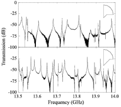
In Fig. 1 we show a part of the spectra of the small and large mushroom billiard, respectively. Details of the experiment with the larger mushroom billiard can be found in friedrich . Three desymmetrized cavities with the shape of billiards from the family of Limaçon billiards have been constructed for the values $\lambda={0.125,0.150,0.300}$ and the first 1163, 1173 and 942 eigenvalues were measured, respectively. More details on these experiments are given in rehfeld ; hesse . To compare the statistical properties of the eigenvalues with universal predictions considered in the present paper, they have to be rescaled to unit mean spacing. This is done by an unfolding procedure using Weyl’s formula Weyl , which relates the billiard area and circumference to the number of resonance frequencies below a given one.

As outlined above, the phase space structure of the billiards with mixed dynamics are different for the two families under consideration. The experimental NNSD of the larger of the two mushroom billiards exhibits friedrich a statistically significant dip at $s\approx 0.7$. It vanishes when the contribution of the two shortest periodic orbits is subtracted. Such a dip has never been observed in the spectra of other billiards with mixed dynamics, including the Limaçon billiards considered here. We shall show below that nevertheless the statistical properties of the Limaçon billiards are indistinguishable from those of the mushroom billiards after removal of the contribution of these periodic orbits, in spite of the difference of their phase space structure.

III Time-series representation

In this section the time series method used for the study of the fluctuations of the resonance spectra of the mushroom billiards is introduced. Representing energy levels of a quantum system as a discrete time series has been probed in a number of recent publications. Relaño et al. relano considered a sequence of energy levels as a discrete time series in which the energy played the role of time. They conjectured that the power spectra of chaotic quantum systems are characterized by $1/f$ noise, whereas integrable quantum systems exhibit $1/f^{2}$ noise. This conjecture was supported by numerical experiments which involved classical random-matrix ensembles and atomic nuclei. Moreover, the power spectrum of an experimentally modeled quantum Sinai billiard exhibits a clear $1/f$ noise through almost the whole frequency domain. Mixed systems on the other hand, like the Limaçon billiard, the quartic coupled oscillator, and the kicked top, are characterized by a $1/f^{\alpha}$ noise gomez ; santhanam . In all these cases, the exponent $\alpha$ was related to the degree of chaos. Manimaran et al. manimaran recently developed a wavelet based approach to discrete time series and employed it to characterize the scaling behavior of spectral fluctuations of random matrix ensembles, as well as complex atomic systems. Santhanam et al. santhanam1 studied the spectra of atoms and Gaussian ensembles using the detrended fluctuation analysis, which is a popular tool to study long range correlations in time series peng . They showed that this analysis is related to the $\Delta_{3}$ statistics of RMT.

Here we apply the time-series analysis to the study of the energy spectra of mixed systems from another point of view. Our goal is to test the hypothesis that quantum systems can be modeled by a generalization of RMT sust1 ; sust2 based on the concept of superstatistics BC . We follow an approach recently proposed by Beck, Cohen and Swinney bcs , which describes how to proceed from a given experimental time series to a superstatistical description. This approach allows one to check whether a time series contains two separate time scales, and also to extract the relevant probability densities of superstatistical parameters from the time series.

III.1 Spectral relaxation lengths

Superstatistical RMT assumes that the space of matrix elements consists of many spatial cells with different values of some intensive parameter, e.g. the inverse variance $\eta$. In systems with mixed regular-chaotic dynamics, the origin of this spectral heterogeneity is the possible partial conservation of an unknown or ignored symmetry. In the space of matrix elements each heterogeneous domain comprises those matrix elements that couple states, which have similar properties with respect to this symmetry, where the typical size of the heterogeneous cells $T$ measures the correlation length in that space. The heterogeneity of the space of matrix elements presumably causes one in the structure of the spectrum. Each cell is assumed to reach local equilibrium very fast, i.e., the associated relaxation length $\tau$, which is defined as that length-scale over which energy fluctuations are correlated, is short. It may also be regarded as an operational definition for the average energy separation between levels due to level repulsion. In the long-term run, the stationary distributions of this inhomogeneous system arise as a superposition of the ”Boltzmann factors” of the standard RMT, i.e. $e^{-\eta\text{Tr}H^{2}}$. The parameter $\eta$ is approximately constant in each cell for an eigenvalue interval of length $T$. In superstatistics this superposition is performed by weighting the stationary distribution of each cell with the probability density $f(\eta)$ to observe some value $\eta$ in a randomly chosen cell and integrating over $\eta$. Of course, a necessary condition for a superstatistical description to make sense is the condition $\tau\ll T$, because otherwise the system is not able to reach local equilibrium before the next change takes place.

Our goal is to show that the behavior of a fictitious time series formed by the 780 and 938 resonances, respectively, in the two mushroom billiards, and the approximately 1100 resonances in each of the three Limaçon billiards is consistent with superstatistics. For this purpose the distribution $f(\eta)$ is derived by proceeding as in bcs . We extract the relaxation lengths (times) to local equilibrium $\tau$ and the large length scale $T$ on which the intensive parameter fluctuates and show that there is a clear scale separation of the spectral correlations in each billiard.

First, let us determine the long time scale $T$. For this we divide the spacings series into $N$ equal level-number intervals of size $n$. The total length of the spectrum is $N\cdot n$. We then define the mean local kurtosis $\kappa(n)$ of a spacing interval of length $n$ by

$$\kappa(n)=\frac{1}{N}\sum_{i=1}^{N}\frac{\left\langle(s-\overline{s})^{4}\right\rangle_{i,N}}{\left\langle(s-\overline{s})^{2}\right\rangle_{i,N}^{2}}.$$ (4)

Here $\left\langle\cdots\right\rangle_{i,N}=\sum_{k=(i-1)\cdot n+1}^{i\cdot n}\cdots$ denotes a summation over an interval of length $n$ starting at level spacing $in$, and $\overline{s}$ is either the local average spacing in each spacing interval or the global average $\overline{s}=1$ over the entire spacings series. We chose the latter one. In probability theory and statistics, kurtosis is a measure for the ”flatness” of the probability distribution of a real-valued random variable. Higher kurtosis means that a larger part of the contributions to the variance is due to infrequent extreme deviations, as opposed to frequent modestly sized ones. A superposition of local Gaussians with local flatness three results in a kurtosis of three. We define the superstatistical level-number scale $T$ by the condition

$$\kappa(T)=3,$$ (5)

that is, we look for the simplest superstatistics, a superposition of local Gaussians bcs . If $n$ is chosen such, that only one value of $s$ is contained in each interval, then of course $\kappa(1)$ =1. If on the other hand $n$ comprises the entire spacing series, then we obtain the flatness of the distribution of the entire signal, which will be larger than 3, since superstatistical distributions are fat-tailed. Therefore, there exists a level-number scale $T$ which solves Eq. (5). Figure 2 shows the dependence of the local flatness of a spacing interval on its length for the two mushroom and the three Limaçon billiards.

Figure 2: The local kurtosis of the spacing intervals of the mushroom (left panel) and Limaçon (right panel) billiards.

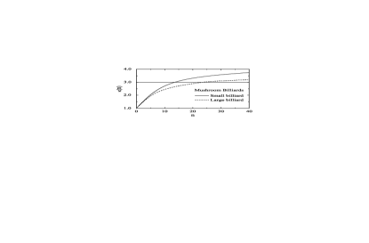
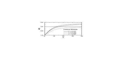
In the case of the chaotic Limaçon billiard, in which $\lambda=0.300,$ the quantity $\kappa$ does not cross the line of $\kappa=3$ for the considered values of $n$. It is expected that $T=N$ in this case since the fluctuations in a chaotic (unfolded) spectrum are uniform. The values of $T$ for the mixed billiards are given in Table 3.

Table 1: Correlation lengths estimated from the time series representing the frequency spectra of the mushroom and Limaçon billiards.

	Mushroom		Limaçon
	small	large	$\lambda=0.125$	$\lambda=0.150$	$\lambda=0.300$
Long-range correlation time
$T$	12.2	23.5	12.3	15.4	large
Short-range correlation times
$\tau_{1}$	0.40	0.03	0.51	0.44	0.02
$\tau_{2}$	1.55	1.12	1.9	2.01	1.36

The short time scale, that is the relaxation time associated with each of the $N$ intervals, was estimated in bcs from the small-argument exponential decay of the autocorrelation function

$$C_{s}(n)=\frac{\overline{s(i)s(i+n)}-1}{\overline{s^{2}}-1}$$ (6)

of the time series $s(t)$ under consideration. Figure 3 shows the behavior of the autocorrelation functions for the series of resonance-spacings of the two families of billiards.

Figure 3: The autocorrelation of the spacings within spectral intervals for the mushroom (left panel) and Limaçon (right panel) billiards.

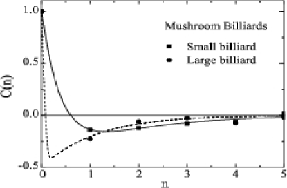
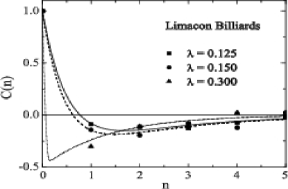
Quite frequently, the autocorrelation function shows single-exponential decays,$\ C(n)=e^{-n/\tau}$, where $\tau>0$ defines a relaxation ”time”. A typical example is the velocity correlation of Brownian motion reif . The autocorrelation functions studied here clearly do not follow this trend. For the systems with mixed dynamics, they decay rapidly from a value of $C(0)=1$, change sign at some $n\sim 1$ becoming negative, then asymptotically tend to zero. In an attempt to quantify the dependence of $C_{s}$ on $n$, we parametrized its empirical value in the form of a superposition of two exponentially decaying functions

$$C_{s}(n)=A_{1}e^{-n/\tau_{1}}+A_{2}e^{-n/\tau_{2}}$$ (7)

and (arbitrarily) fixed the superposition coefficient as $A_{1}=1.5$ and $A_{2}=-0.5.$ The curves in Fig. 3 show the resulting parametrization. The best fit parameters are given in Table 3. We may estimate $\tau$ as the mean values of $\tau_{1}$ and $\tau_{2}$ and conclude that $\tau$ has a value slightly larger than 1 for each billiard. This is sufficient to conclude that the ratio $T/\tau$ is large enough in each billiard to claim two well separated ”time” scales in the level-spacings series, which justifies describing them within the framework of superstatistics.

Both Figs. 2 and 3 as well as Table  suggest that the evolution of the quantities $\kappa(n)$ and $C_{s}(n)$ along the time series for the two billiard families is the same despite the different behavior of their classical dynamics.

III.2 Estimation of the parameter distribution

The distribution $f(\eta)$ is determined by the spatiotemporal dynamics of the entire system under consideration. Beck et al. bcs have argued that typical experimental data are described by one of three superstatistical universality classes, namely, $\chi^{2}$, inverse $\chi^{2}$, or log-normal superstatistics. The first is the appropriate one if $\eta$ has contributions from $\nu$ Gaussian random variables $X_{1}$, . . . , $X_{\nu}$ due to various relevant degrees of freedom in the system. As mentioned before $\eta$ needs to be positive; this is achieved by squaring these Gaussian random variables. Hence, $\eta=\sum_{i=1}^{\nu}X_{i}^{2}$ is $\chi^{2}$ distributed with degree $\nu$,

$$f(\eta)=\frac{1}{\Gamma(\nu/2)}\left(\frac{\nu}{2\eta_{0}}\right)^{\nu/2}\eta^{\nu/2-1}e^{-\nu\eta/2\eta_{0}}.$$ (8)

The average of $\eta$ is $\eta_{0}=\int_{0}^{\infty}\eta f(\eta)d\eta$. The same considerations are applicable if $\eta^{-1},$ rather than $\eta,$ is the sum of several squared Gaussian random variables. The resulting distribution $f(\eta)$ is the inverse $\chi^{2}$ distribution given by

$$f(\eta)=\frac{\eta_{0}}{\Gamma(\nu/2)}\left(\frac{\nu\eta_{0}}{2}\right)^{\nu/2}\eta^{-\nu/2-2}e^{-\nu\eta_{0}/2\eta},$$ (9)

where again $\eta_{0}$ is the average of $\eta$. Instead of being a sum of many contributions, the random variable $\eta$ may be generated by multiplicative random processes. Then $\ln\eta=\sum_{i=1}^{\nu}\ln X_{i}$ is a sum of Gaussian random variables. Thus it is log-normally distributed,

$$f(\eta)=\frac{1}{\sqrt{2\pi}v\eta}e^{-\left.\left[\ln(\eta/\mu)\right]^{2}\right/2v^{2}},$$ (10)

which has an average $\mu\sqrt{w}$ and variance $\mu^{2}w(w-1)$, where $w=\exp(v^{2})$.

Next, we need to determine which of these distributions fits best that of the slowly varying stochastic process $\eta(t)$ described by the experimental data. Since the variance of superimposed local Gaussians (see remark after Eq. (5)) is given by $\eta^{-1}$, we may determine the process $\eta(t)$ from the series

$$\eta(i)=\frac{1}{\left\langle s^{2}\right\rangle_{i,T}-\left\langle s\right\rangle_{i,T}^{2}}.$$ (11)

Accordingly, the probability density $f(\eta)$ is determined from the histogram of the $\eta\left(i\right)$ values for all $i$; the resulting experimental distributions are shown in Fig. 4.

Figure 4: Estimation of the parameter distribution for the superstatistical description of spectra of the mushroom (left panel) and Limaçon (right panel) billiards. The solid lines represent the $\chi^{2}$, the daotted lines the inverse $\chi^{2}$ and the dashed lines the log-normal distribution.

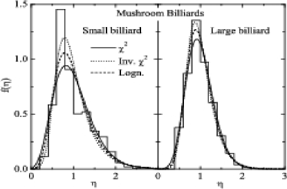
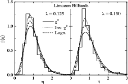
We compared them with the log-normal, the $\chi^{2}$ and the inverse $\chi^{2}$ distributions with the same mean $\left\langle\eta\right\rangle$ and variance $\left\langle\eta^{2}\right\rangle-\left\langle\eta\right\rangle^{2}$. The inverse $\chi^{2}$ distribution fits the data significantly better than the other two distributions.

IV Nearest-neighbor spacing distribution

This section focusses on the question whether the inverse $\chi^{2}$ distribution of the superstatistical parameter $\eta$ in Eq. (9) is suitable for describing the NNSD of systems in the transition out of chaos within the superstatistical approach to RMT. As mentioned above, the NNSD of a chaotic system is well described by that of random matrices from the GOE, the Wigner surmise, if the system is chaotic and by that for Poisson statistics if it is integrable. Numerous interpolation formulas describing the intermediate situation between integrability and chaos have been proposed guhr . One of the most popular ones is that introduced by Brody brody although it is purely phenomenological. This distribution coincides with the Wigner distribution for a fully chaotic and with Poisson’s for an integrable system. It is known to provide an excellent description for the NNSDs of numerous mixed systems. Another phenomenological distribution was proposed in casati and its usefulness was demonstrated for band random matrices. Lenz and Haake lenz derived a distribution based on the model of additive random matrices. Finally, Berry and Robnik elaborated a NNSD for mixed systems based on the assumption that semiclassically the eigenfunctions and associated Wigner distributions are localized either in classically regular or chaotic regions in phase space berryrobnik . Accordingly, the sequences of eigenvalues connected with these regions are assumed to be statistically independent, and their mean spacing is determined by the invariant measure of the corresponding regions in phase space. The largest discrepancy between the Brody and the Berry-Robnik distribution is observed for level spacings $s$ close to zero. While the former vanishes for $s=0$, the latter approaches a constant and nonvanishing value for $s\to 0$. In friedrich ; rehfeld the experimental NNSDs for the measured resonance frequencies of the mushroom and the Limaçon billiards, respectively, were compared to the Berry-Robnik (BR) distribution.

It follows from Eq. (2) that the statistical measures of the eigenvalues of the superstatistical ensemble are obtained as an average of the corresponding $\eta$-dependent ones of standard RMT weighted with the parameter distribution $f(\eta)$. In particular, the superstatistical NNSD is given by sust1 as

$$p(s)=\int_{0}^{\infty}f(\eta)~{}p_{\text{W}}(\eta,s)~{}d\eta,$$ (12)

where $p_{\text{W}}(\eta,s)$ is the Wigner surmise for the Gaussian orthogonal ensemble with the mean spacing depending on the parameter $\eta$,

$$p_{\text{W}}(\eta,s)=\eta s\exp\left(-\frac{1}{2}\eta s^{2}\right).$$ (13)

For a $\chi^{2}$ distribution of the superstatistical parameter $\eta$, one substitutes Eq. (8) into Eq. (13) and integrates over $\eta.$ The resulting NNSD is given by

$$p_{\chi^{2}}(\nu,s)=\frac{\eta_{0}s}{(1+\eta_{0}s^{2}/\nu)^{1+\nu/2}}.$$ (14)

The parameter $\eta_{0}$ is fixed by requiring that the mean-level spacing $\left\langle s\right\rangle$ equals unity, yielding

$$\eta_{0}=\frac{\pi\nu}{4}\left[\left.\Gamma\left(\frac{\nu-1}{2}\right)\right/\Gamma\left(\frac{\nu}{2}\right)\right]^{2}.$$ (15)

For an inverse $\chi^{2}$ distribution of $\eta$, given by Eq. (9), one obtains the following superstatistical NNSD,

$$p_{\,\text{Inv}\,\chi^{2}}(\nu,s)=\frac{2\eta_{0}s}{\Gamma\left(\nu/2\right)}\left(\sqrt{\eta_{0}\nu}s/2\right)^{\nu/2}\\ K_{\nu/2}\left(\sqrt{\eta_{0}\nu}s\right),$$ (16)

where $K_{m}(x)$ is a modified Bessel function grad and $\eta_{0}$ again is determined by the requirement that the mean-level spacing $\left\langle s\right\rangle$ equals unity,

$$\eta_{0}=\frac{4\pi}{\nu^{3}}\left[\left.\Gamma\left(\frac{3+\nu}{2}\right)\right/\Gamma\left(\frac{\nu}{2}\right)\right]^{2}.$$ (17)

Finally, if the parameter $\eta~{}$has a normal distribution (10), then the NNSD

$$p_{\text{\,logn}}(v,s)=\frac{s}{\sqrt{2\pi}v}\int_{0}^{\infty}\exp\left[-\frac{\eta s^{2}}{2}-\frac{\ln^{2}\left(\frac{2}{\pi}\eta e^{-v^{2}/4}\right)}{2v^{2}}\right]d\eta$$ (18)

can only be evaluated numerically.

We compared the resulting NNSDs given in Eqs. (14), (16) and (18) with the experimental ones for the mushroom billiards and the two Limaçon billiards with mixed dynamics. In Fig. 5 the experimental results are shown together with the superstatistical and the BR distributions.

Figure 5: Experimental NNSDs for the mushroom (left panel) and Limaçon (right panel) billiards compared with the superstatistical distributions. The solid lines represent the $\chi^{2}$, the dashed lines the inverse $\chi^{2}$, the dashed lines the log-normal and the short-dashed lines the Berry-Robnik distribution.

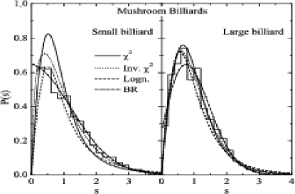
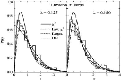
The best fit values of the parameters are given in Table 2.

Table 2: Best-fit parameters for the experimental NNSD and resonance-strength distributions in the mixed billiards. The corresponding $\chi^{2}$-values are given in brackets.

	Mushroom		Limaçon
	small	large	$\lambda=0.125$	$\lambda=0.150$
NNSD
$\chi^{2}$	$\nu=2.95$ (0.0189)	$\nu=6.03$ (0.0031)	$\nu=2.57$ (0.0133)	$\nu=2.63$ (0.0097)
Inverse-$\chi^{2}$	$\nu=0.00$ (0.0042)	$\nu=2.31$ (0.0018)	$\nu=0.00$ (0.0031)	$\nu=0.00$ (0.0021)
Log-normal	$v=1.41$ (0.0129)	$v=0.96$ (0.0033)	$v=1.23$ (0.0104)	$v=1.17$ (0.0078)
Berry-Robnik	$q=0.24$ (0.0007)	$q=0.87$ (0.0027)	$q=0.58$ (0.0020)	$q=0.62$ (0.0034)
Resonance strength distribution
$\chi^{2}$			$\nu=2.66$ (0.00142)	$\nu=3.47$ (0.00035)
Inverse-$\chi^{2}$			$\nu=0.50$ (0.00030)	$\nu=0.98$ (0.00045)
Gamma distribution			$\nu=0.76$ (0.00120)	$\nu=0.81$ (0.00131)

We in addition used the entropy Kullback ; barbosa

$$S(P\left|p\right)=-\int P(x)\ln\frac{P(x)}{p(x)}dx$$ (19)

to express the difference between the theoretical Ansatz $p(x)$ and the experimental distribution $P(x)$. Such a reference term has been discussed in the literature in the context of going from a discrete to a continuous system and is proportional to the limiting density of discrete points Jaynes . As is well known, the entropy $S(P\left|p\right)$ is negative everywhere except at its maximum, where it equals zero and $P(x)=p(x)$. One can use this fact to find the value of the parameter of a theoretical distribution that has the least distance to the experimental distribution. The resulting best fit values of the parameters are given in Table 3.

Table 3: Best-fit parameters obtained by extremizing the relative entropy for the experimental NNSDs the mixed billiards. The corresponding values of the relative entropy are given in brackets.

	Mushroom		Limaçon
	small	large	$\lambda=0.125$	$\lambda=0.150$
NNSD
$\chi^{2}$	$\nu=2.67$ (-0.0920)	$\nu=7.93$ (-0.0232)	$\nu=2.62$ (-0.0909)	$\nu=2.69$ (-0.0827)
Inverse-$\chi^{2}$	$\nu=0.01$ (-0.0353)	$\nu=3.14$ (-0.0175)	$\nu=0.01$ (-0.0341)	$\nu=0.01$ (-0.0362)
Log-normal	$v=1.31$ (-0.0568)	$v=0.60$ (-0.0206)	$v=1.33$ (-0.0533)	$v=1.26$ (-0.0537)
Berry-Robnik	$q=0.55$ (-0.0289)	$q=0.87$ (-0.0203)	$q=0.57$ (-0.0293)	$q=0.58$ (-0.0378)

Figure 5 and Tables 2 and 3 suggest the validity of the superstatistical distribution, especially for the nearly chaotic billiards. It clearly shows that the NNSD for the inverse $\chi^{2}$ distribution $p_{\,\text{Inv}\,\chi^{2}}(\nu,s)$ agrees in a similar or, especially for small spacings, even better quality with the experimental ones as the others including the Brody (not shown) and the BR distribution.

The distribution $p_{\,\text{Inv}\,\chi^{2}}(\nu,s)$ (see Eq. (16)) coincides with the Wigner distribution in the limit of $\nu\rightarrow\infty.$ As $\nu$ decreases, the distribution evolves towards a well-defined limit, but this limiting case does not resemble the Poisson distribution as one would expect. To demonstrate this behavior and give a feeling for the size of the tuning parameter $\nu,$ we evaluate its value corresponding to the minimal deviation from a BR distribution with a given degree of chaoticity $q$. For this we define a measure

$$d_{\,\text{Inv}\,\chi^{2},\text{BR}}(\nu,q)=\min{\int_{0}^{\infty}\left[p_{\,\text{Inv}\,\chi^{2}}(\nu,s)-p_{\text{BR}}(q,s)\right]^{2}ds}.$$ (20)

The distance $d_{\,\text{Inv}\,\chi^{2},\text{BR}}$ between the two distributions equals zero for $q=1$ and $\nu\rightarrow\infty$, where both distributions coincide with the Wigner distribution. Its value increases on departure from these parameter values, has a maximum value of 0.0030 for $\nu=1$ and then decreases to a value of 0.0025 at $\nu=0$. The measure $d_{\,\text{Inv}\,\chi^{2},\text{BR}}(\nu,q)$ yields a relation between the BR and the superstatistical parameter $\nu$, which is shown in Fig. 6.

Figure 6: The relation between the tuning parameters $q$ and $\nu$ of the Berry-Robnik and superstatistical NNSDs, respectively.

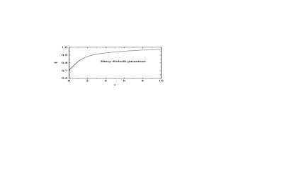
The figure suggests that $p_{\,\text{Inv}\,\chi^{2}}(\nu,s)$ can only describe the initial stage of the transition from chaos to regularity. One can find a BR distribution that agrees well with $p_{\,\text{Inv}\,\chi^{2}}$ until an intermediate situation in which the NNSD corresponds to a Berry-Robnik parameter $q=0.83.$ The failure of spacing distributions interpolating between those describing chaotic and regular systems in the limit of near integrability is common in different RMT descriptions based on generalized statistical mechanics, e.g. in evans ; toscano ; nobre ; abul ; bertuola ; abul1 . As mentioned above, the superstatistical random-matrix ensemble is base invariant. The Hamiltonian of an integrable system, on the other hand, by definition, has a well defined complete set of eigenstates, which constitutes a preferred basis. The RMT approach to mixed systems cannot depart far from the state of chaos without breaking base invariance.

The variance $\sigma^{2}$ of the NNSD is often regarded as a one-parameter interpolation between chaos and order because it monotonically increases from $(4/\pi-1)\cong 0.273$ for the Wigner distribution to 1 for the Poissonian. At $\nu=0$, the superstatistical distribution in Eq. (9) becomes

$$p_{\,\text{Inv}\,\chi^{2}}(0,s)=\frac{\pi^{2}}{4}sK_{0}\left(\frac{\pi}{2}s\right)$$ (21)

and has a variance $\sigma^{2}=\left(16/\pi^{2}-1\right)\cong 0.621$. This value is slightly larger than 0.5 which is exactly the variance of the semi-Poisson distribution

$$p_{\text{SP}}(s)=4s\exp(-2s).$$ (22)

The semi-Poisson distribution was suggested to describe a narrow intermediate region between insulating and conducting regimes exemplified by the Anderson localization model evangelou , with the two limiting cases being described by Poisson and Wigner statistics, respectively. It was introduced to mimic new seemingly universal properties in certain classes of systems, in particular, being characteristics of the “critical quantum chaos”. Figure 7 compares the limiting

Figure 7: The superstatistical NNSD $p_{\,\text{Inv}\,\chi^{2}}(0,s)$ compared with the semi-Poisson distribution $P_{SP}$.

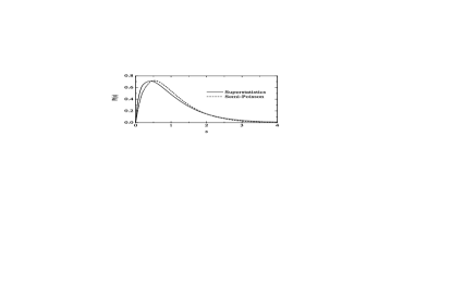
superstatistical distribution,  $p_{\,\text{Inv}\,\chi^{2}}(0,s)$, with the semi-Poisson distribution. We see from the figure that the two distributions are quite similar in shape; the superstatistical distribution seems to just have passed the semi-Poissonian before reaching its final shape for $\nu=0$. Therefore it is worth in the present context to use the semi-Poisson statistics as a reference distribution marking the limit of validity of the base-invariant random-matrix description of mixed systems.

V Resonance strength

In the preceding section we have seen that superstatistics yields a theoretical description of statistical properties of the eigenvalues of a quantum system with mixed classical dynamics, which is of similar quality as existing ones, like e.g. the Brody and the BR ansatz. The great advantage of the method of superstatistics is, that we can similarly apply it to calculate the distribution of the eigenvector components of a Hamiltonian describing a mixed system in which the spectrum is composed of subspectra associated with levels following Poissonian and Wigner statistics sust3 . For a chaotic system the squared eigenvector components follow the Porter-Thomas distribution

$$P_{\text{PT}}(t)=\sqrt{\frac{{\eta}}{\pi y}}e^{-{\eta}t},$$ (23)

where ${\eta}$ is a constant parameter related to the mean value barbosa . In sust3 superstatistics of the transition matrix elements was introduced by representing the transition-intensity distribution as a superposition of Porter-Thomas distributions with different values for the parameter $\eta$. Similarly, in a superstatistical description of the squared eigenvector components of the Hamilton operator or equivalently the partial widths of the resonances of a microwave resonator, the parameter ${\eta}$ in Eq. (23) is no longer considered to be a constant but allowed to fluctuate according to a distribution $f({\eta})$. The superstatistical distribution of the squared eigenvector components is then given by

$$P_{\text{Sst}}(t)=\int_{0}^{\infty}f({\eta})\sqrt{\frac{{\eta}}{\pi t}}e^{-{\eta}t}d{\eta}.$$ (24)

The parameter distribution ${f}({\eta})$ was determined in sust3 using maximum-entropy arguments sattin . There, the resulting expression for the transition intensity distribution was fit to the distributions of the experimental reduced transition probabilities in ²⁶Al and ³⁰P nuclei adamsx ; shriner . It fits the data much better than a $\chi^{2}$ distribution with $\nu$ degrees of freedom, which is given in Eq. (8) with $\eta_{0}=1$ and has been proposed by Alhassid and Novoselsky alhassid  and frequently used for describing the deviation of partial width distributions from the Porter-Thomas distribution. The superstatistical distributions obtained from Eq. (24) for a $\chi^{2}$, inverse $\chi^{2}$ and log-normal distribution $f(\eta)$ (see Eqs. (8)-(10)), respectively, read

$$P_{\chi^{2}}(\nu,t)=\frac{\Gamma\left(\frac{\nu+1}{2}\right)}{\sqrt{\left(\nu-2\right)\pi t}~{}\Gamma\left(\frac{\nu}{2}\right)}\left(\frac{t}{\nu-2}+1\right)^{-(\nu+1)/2},$$ (25)

$$P_{\,\text{Inv}\,\chi^{2}}(\nu,t) = \frac{2^{(1+\nu)/2}(\nu+2)}{\nu~{}\sqrt{\pi}\Gamma\left(\nu/2\right)}\left[t(\nu+2)\right]^{(\nu-1)/4}$$

$$\cdot K_{(1+\nu)/2}\left(\sqrt{t(\nu+2)}\right),$$

and

$$P_{\text{\,logn}}(v,t)=\frac{1}{\sqrt{2t}\pi v}\int_{0}^{\infty}\frac{1}{\sqrt{\eta}}\exp\left[-\eta t-\frac{\ln^{2}\left(2\eta e^{-v^{2}/4}\right)}{2v^{2}}\right]d\eta.$$ (27)

Unfortunately the latter integral could not be evaluated analytically.

In dembo , a new statistics, the resonance strength distribution was introduced. For each resonance, a measurement of the transmission of microwave power from one antenna to another provides the product of the two partial widths related to the antenna “channels”. This product has been named the strength of the resonance with respect to the transmission between the antenna channels. In Ref. dembo the strength distribution was investigated experimentally for all three Limaçon billiards. Altogether four antennas were attached to each of the microwave billiards and the transmission spectra between pairs of antennas (a,b) were measured for all six possible antenna combinations. An analytic expression for the strength distribution of a pair of partial widths with distributions $P_{\text{a}}$ and $P_{\text{b}}$ is obtained as

$$P\left(y\right)=\int_{0}^{\infty}P_{\text{a}}(t_{\text{a}})P_{\text{b}}(t_{\text{b}})\delta(y-t_{\text{a}}t_{\text{b}})dt_{\text{a}}dt_{\text{b}}.$$ (28)

The distribution of the partial widths of a chaotic microwave billiard is well described by the Porter-Thomas distribution Eq. (23), and the corresponding resonance strength distribution is given as

$$P_{\text{GOE}}(y)=\frac{K_{0}\left(\sqrt{y}\right)}{\pi\sqrt{y}}.$$ (29)

More generally, if the partial width distribution is a $\chi^{2}$ distribution as proposed by Alhassid and Novoselsky, then Eqs. (28) and (8) aith $\eta_{0}=1$ yield

$$P_{\text{Alh-Nov}}(\nu,y)=\frac{2^{1-\nu}\left(\nu\sqrt{y}\right)^{\nu}K_{0}\left(\nu\sqrt{y}\right)}{y~{}\Gamma^{2}\left(\nu/2\right)}.$$ (30)

The superstatistical resonance-strength distributions are obtained by substituting the corresponding partial-width distributions (Eqs. (25)-(V)) into Eq. (28). If the parameter $\eta$ has a log-normal distribution this leads to a double-integral which is not easy to calculate. For the case of a $\chi^{2}$ distribution (see Eq. (8)), the resonance-strength distribution is given by

$$P_{\chi^{2}}(\nu,y) = \frac{1}{\left(\nu-2\right)\pi\sqrt{y}~{}\Gamma^{2}\left(\nu/2\right)}\left(\frac{y}{(\nu-2)^{2}}\right)^{-(\nu+1)/2}$$ (31)

$$\cdot G_{22}^{22}\left(\frac{y}{(\nu-2)^{2}}\left|\begin{array}[]{c}1,1\\ \frac{\nu+1}{2},\frac{\nu+1}{2}\end{array}\right.\right)$$ (34)

where $G_{pq}^{mn}\left(x\left|\begin{array}[]{c}a_{1},...,a_{p}\\ b_{1},...,b_{q}\end{array}\right.\right)$ is Meijer’s $G$-function grad ; luke ; wolfram . On the other hand, if the parameter ${\eta}$ has an inverse $\chi^{2}$ distribution, one obtains

$$P_{\,\text{Inv}\,\chi^{2}}(\nu,y) = \frac{(\nu+2)^{2}}{4\pi\nu^{2}~{}\Gamma^{2}\left(\nu/2\right)}$$

$$\cdot G_{04}^{40}\left(\frac{1}{16}(\nu+2)^{2}y\left|-\frac{1}{2},-\frac{1}{2},\frac{\nu}{2},\frac{\nu}{2}\right.\right).$$

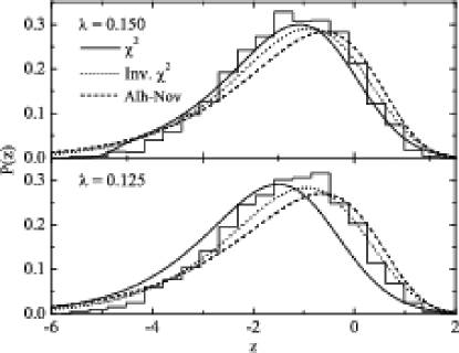
Figure 8 compares the experimental resonance strength distributions for the

Figure 8: The resonance strength distributions in the mixed Limaçon billiards compared with the predictions of different superstatistics. The solid lines represent the $\chi^{2}$, the dashed lines the inverse $\chi^{2}$ distribution, while the short-dashed line corresponds to the case in which the strengths have a $\chi^{2}$ distribution.

two mixed Limaçon billiards, expressed as functions of $z$ = log₁₀ $y$, with the corresponding distribution given in Eqs. (30), (34) and (V). The best-fit values of the parameters are given in Table2. Both cases demonstrate the superiority of the superstatistical inverse $\chi^{2}$ distribution.

VI SUMMARY

Superstatistics has been applied to the study of a wide range of phenomena from turbulence to topics in econophysic. RMT of the Gaussian ensembles is among these. In its application, the variance of the distribution of the matrix elements is chosen as a parameter whose distribution is obtained by assuming a suitable form or applying the principle of maximum entropy. In this paper we use the time-series method to show that the spectra of mixed systems have two correlation scales as required for the validity of the superstatistical approach. The time-series analysis also shows that the best choice of the superstatistical parameter distribution for a mixed system is an inverse $\chi^{2}$ distribution. We computed the corresponding NNSD of the energy levels and compared it with the spectrum of two microwave resonators of mushroom-shaped boundaries and two of the family of Limaçon billiards, which exhibit mixed regular-chaotic dynamics. The agreement is found to be similar to that with all the other considered well-established distributions including the celebrated BR distribution. The method of superstatics also provides a description of statistical properties of the eigenfunctions of a system with mixed classical dynamics. Thus, the resonance-strength distributions for the Limaçon billiards could be analyzed. The agrreement with the experimental resonance-strength distributions is better than with that derived from the Alhassid-Novoselsky $\chi^{2}$ distribution of transition intensities.