Quasifermion spectrum at finite temperature from coupled Schwinger-Dyson equations for a fermion-boson system

Abstract

We nonperturbatively investigate a fermion spectrum at finite temperature in a chiral invariant linear sigma model. Coupled Schwinger-Dyson equations for fermion and boson are developed in the real time formalism and solved numerically. From the coupling of a massless fermion with a massive boson, the fermion spectrum shows a three-peak structure at some temperatures even for the strong coupling region. This means that the three-peak structure which was originally found in the one-loop calculation is stable against higher order corrections even in the strong coupling region.

I Introduction

One of unexpected experimental discoveries in heavy-ion collisions at the Relativistic Heavy Ion Collider (RHIC) is that the created matter could be close to a perfect fluidArsene:2004fa . Then, considerable changes have occurred with our understanding of quark-gluon plasma (QGP), which is now believed to be rather strongly coupled or strongly interacting just above the critical temperature ($T_{c}$) of the chiral and deconfinement transitions, $T\gtrsim T_{c}$. Nonperturbative results from lattice QCD seem to support this view: The lowest charmonium state survives for $T\gtrsim T_{c}$, which suggests strong correlations between quarksAsakawa:2003re . Furthermore, very small viscosity-entropy ratio suggested from RHIC experiments is consistent with the result of the strongly coupled supersymmetric Yang-Mills theory based on the analysis with the AdS/CFT correspondenceKovtun:2004de .

The present paper is concerned with spectral properties of fermions in such a strongly coupled system, because quarks are the basic degrees freedom of the created matter in the deconfined phase together with gluons at RHIC. It is not even clear whether quarks manifest themselves as well-defined quasiparticles in such a system. So far, there exist some theoretical investigations on this issueSchaefer:1998wd ; Mannarelli:2005pz . Recently, the thermal mass of the quark near $T_{c}$ was studied in quenched lattice QCD and was fitted well with a two-pole ansatzKarsch:2007wc . The authors and Yoshimoto investigated the quasiquark spectrum with a strong coupling gauge theory based on the Schwinger-Dyson equation (SDE) and found that the thermal mass is of the order $T$ and depends on the coupling little in the strong coupling regionHarada:2007gg . In Ref. Kitazawa:2005mp , it is shown in the Nambu–Jona-Lasinio model that the quark spectrum has three peaks near $T_{c}$, which result from the coupling with fluctuations of the chiral condensateHatsuda:1985eb .

The above peculiar three-peak structure of the quark spectrum is then found to be rather generic at finite $T$: It is due to the coupling with massive bosonic modes through the Landau damping, which was analyzed in detail in Yukawa models at one loopKitazawa:2006zi ; Kitazawa:2007ep . While the three-peak structure appears most clearly for the massless fermion, it even appears for small massive fermionsKitazawa:2007ep . One of the remained issues is whether it is stable against higher order effects. One of the purposes of this paper is to study it in a linear sigma model by incorporating nonperturbative effects with the SDERoberts:2000aa . It is shown in Ref. Kitazawa:2006zi that for the massless fermion, the three-peak structure appears independently of the coupling over some range of $T$ at the one-loop order. Because the SDE should reproduce the perturbation theory in the weak coupling region, the three-peak structure would remain there even in this approach. However, it is quite nontrivial whether it still appears in the strong coupling region where higher order effects are not negligible.

Another purpose of this study is to formulate coupled SDE for fermion and boson at finite $T$. In the past approaches, the boson propagator was not solved self-consistently, but fixed at the beginningBarducci:1989eu ; Kondo:1993pd ; Taniguchi:1995vf ; Blaschke:1997bj ; Harada:1998zq ; Ikeda:2001vc ; Takagi:2002vj ; Harada:2007gg ; Nakkagawa:2007ti . As far as we know, this paper gives the first numerical result for the coupled SDE for a fermion-boson system at finite $T$. The point in our formulation is that while the imaginary parts of the self-energies are evaluated through loop integrals, the real parts are evaluated from the imaginary parts with the dispersion relation which is a one-dimensional integral, and thus the computation is much faster than that of the four-dimensional loop integral. This reduction of the computational cost makes it possible to solve the coupled SDE for fermion and boson quite fast.

The content of this paper is as follows. We employ a linear sigma model in the chiral symmetric phase to study the fermion spectrum at finite $T$. In Sec. II, the model is introduced and the SDE are formulated using the real time formalism. We use the ladder approximation to construct the SDE in which the bare vertex is used for the self-energies. Then, the renormalization is carried out for the boson mass and some remarks are made for the triviality of the model. In Sec. III, some numerical results of the fermion spectral functions are shown, focusing on the $T$ and coupling dependences and nonperturbative effects by comparing with the results in the one-loop calculation. Concluding remarks and outlook are given in Sec. IV.

II Schwinger-Dyson equations at finite temperature

Figure 1: Self-energies for fermion (left) and boson (right). Solid lines denote the fermion propagator and dashed lines the boson propagator.

We consider a U(1)${}_{L}\times$ U(1)_R invariant linear sigma model with Dirac fermions,

$$\mathcal{L}=\bar{\psi}i\partial/\psi+\frac{1}{2}\partial_{\mu}M^{*}\partial^{\mu}M-\frac{m_{0}^{2}}{2}M^{*}M+g[\bar{\psi}_{L}M\psi_{R}+\bar{\psi}_{R}M^{*}\psi_{L}],$$ (1)

where $M=\phi_{1}+i\phi_{2}$ and $\phi_{1}(\phi_{2})$ denotes a scalar (pseudoscalar) boson field. Because our motivation lies in the quark spectrum in the QGP phase with possible bosonic excitations, we assume $m_{0}^{2}>0$, i.e. the chiral symmetry is not spontaneously broken. Self-coupling terms of the boson fields are not introduced for simplicity. Their main effect is to shift the thermal mass and the width of the boson spectrum. As mentioned below, we renormalize the thermal mass of the boson and measure all the dimension-full quantities in units of the renormalized boson mass. Then, effects of the self-coupling of the bosons are not important for the fermion spectrum. Although we consider a chiral U(1)${}_{L}\times$ U(1)_R symmetry for simplicity, an extension to the SU(2)${}_{L}\times$ SU(2)_R symmetry is trivial as mentioned below also.

II.1 Formulation of the Schwinger-Dyson equations

To construct the SDE, we employ the real time formalism. It is convenient to use the following Green functions,

$$iS^{>}(x,y) =\langle\psi(x)\bar{\psi}(y)\rangle,\quad iS^{<}(x,y)=\langle\bar{\psi}(y)\psi(x)\rangle,$$

$$iG_{i}^{>}(x,y) =\langle\phi_{i}(x)\phi_{i}(y)\rangle,\quad iG_{i}^{<}(x,y)=\langle\phi_{i}(y)\phi_{i}(x)\rangle,\quad(i=1,2).$$ (2)

Because we consider the chiral symmetric phase, there is no difference between $G_{1}^{\gtrless}$ and $G_{2}^{\gtrless}$, and thus we simply write them as $G^{\gtrless}$ in the following.

We formulate the SDE in the ladder approximation whose self-energies are depicted in Fig. 1. The fermion self-energy reads

$$\Sigma(x,y)=\theta_{c}(x^{0}-y^{0})\Sigma^{>}(x,y)-\theta_{c}(y^{0}-x^{0})\Sigma^{<}(x,y),$$ (3)

where

$$\Sigma^{\gtrless}(x,y)=-2g^{2}iS^{\gtrless}(x,y)G^{\gtrless}(x,y),$$ (4)

and $\theta_{c}$ denotes the step function along the closed time path in the real time formalismLeB . The factor 2 in Eq. (4) comes from the number of boson fields, $\phi_{1}$ and $\phi_{2}$. Thus, for the SU(2)${}_{L}\times$ SU(2)_R invariant linear sigma model, this factor is replaced by 4, which is the only difference between the U(1)${}_{L}\times$ U(1)_R model and the SU(2)${}_{L}\times$ SU(2)_R model in the fermion self-energy. The boson self-energy reads

$$\Pi(x,y)=\theta_{c}(x^{0}-y^{0})\Pi^{>}(x,y)+\theta_{c}(y^{0}-x^{0})\Pi^{<}(x,y),$$ (5)

where

$$\Pi^{\gtrless}(x,y)=-g^{2}i\textrm{Tr}[S^{\gtrless}(x,y)S^{\lessgtr}(y,x)],$$ (6)

and Tr means the trace for the Dirac index. For the SU(2)${}_{L}\times$ SU(2)_R invariant model, a factor 2 coming from the trace in the flavor index is multiplied in Eq. (6).

In equilibrium, we can Fourier-transform the above functions using the translation invariance. In momentum space, the Green functions $S^{\gtrless}(G^{\gtrless})$ have simple expressions with the spectral function $\rho_{f}(\rho_{b})$ and the Fermi-Dirac (Bose-Einstein) distribution function $f(n)$,

$$iS^{>}(p^{0},\bm{p}) =[1-f(p_{0})]\rho_{f}(p_{0},\bm{p}),\quad iS^{<}(p^{0},\bm{p})=f(p^{0})\rho_{f}(p^{0},\bm{p}),$$ (7)

$$iG^{>}(p^{0},\bm{p}) =[1+n(p_{0})]\rho_{b}(p_{0},\bm{p}),\quad iG^{<}(p^{0},\bm{p})=n(p^{0})\rho_{b}(p^{0},\bm{p}).$$ (8)

Using these expressions, the self-energies in momentum space are written as

$$\Sigma_{\rho}(P) \equiv i\Sigma^{>}(P)+i\Sigma^{<}(P)$$

$$=-2g^{2}\int\frac{d^{4}Q}{(2\pi)^{4}}[1-f(q^{0})+n(p^{0}-q^{0})]\rho_{f}(Q)\rho_{b}(P-Q),$$ (9)

$$\Pi_{\rho}(P) \equiv i\Pi^{>}(P)-i\Pi^{<}(P)$$

$$=-4g^{2}\int\frac{d^{4}Q}{(2\pi)^{4}}[1-f(q^{0})-f(p^{0}-q^{0})]\rho_{f}^{\mu}(Q)\rho_{f\mu}(P-Q),$$ (10)

with $P=(p^{0},\bm{p}),\,Q=(q^{0},\bm{q}),\,\rho_{f}^{\mu}=(\rho^{0}_{f},\mbox{\boldmath$\rho$}_{f})$ and $\rho_{f}=\gamma_{0}\rho^{0}_{f}-\mbox{\boldmath$\gamma$}\cdot\mbox{\boldmath$\rho$}_{f}$. The functions $\Sigma_{\rho}$ and $\Pi_{\rho}$ are related to the corresponding retarded self-energies,

$$\textrm{Im}\Sigma^{R}(P) =-\frac{1}{2}\Sigma_{\rho}(P),\quad\textrm{Re}\Sigma^{R}(P)=\textrm{P}\int\frac{dq^{0}}{2\pi}\frac{\Sigma_{\rho}(q^{0},\bm{p})}{p^{0}-q^{0}},$$

$$\textrm{Im}\Pi^{R}(P) =-\frac{1}{2}\Pi_{\rho}(P),\quad\textrm{Re}\Pi^{R}(P)=\textrm{P}\int\frac{dq^{0}}{2\pi}\frac{\Pi_{\rho}(q^{0},\bm{p})}{p^{0}-q^{0}},$$ (11)

where P denotes the principal integral.

The retarded Green functions are expressed with the retarded self-energies and thus $\Sigma_{\rho}$ and $\Pi_{\rho}$ as

$$S^{R}(P) =\frac{1}{P/+\textrm{Re}\Sigma^{R}(P)+i\textrm{Im}\Sigma^{R}(P)},$$

$$G^{R}(P) =\frac{1}{P^{2}-m_{0}^{2}+\textrm{Re}\Pi^{R}(P)+i\textrm{Im}\Pi^{R}(P)}.$$ (12)

The spectral functions are in turn expressed with the retarded Green functions,

$$\rho_{f}(P) =-2\textrm{Im}S^{R}(P),\quad\rho_{b}(P)=-2\textrm{Im}G^{R}(P).$$ (13)

Equations (9)-(13) are closed form for the spectral functions $\rho_{f}$ and $\rho_{b}$, and thus give the self-consistency condition.

Two comments are in order.

One is that this formulation is similar to that given in Appendix D of Ref.Juchem:2003bi . The main difference is in the calculation method of the self-energies: While we evaluate them as momentum integrals, in Ref.Juchem:2003bi the self-energies are Fourier-transformed and evaluated in the coordinate space. In the latter, the fast Fourier transformation algorithm can be used for the numerical calculation and in general is faster than the direct evaluation of the four-dimensional integral. In equilibrium, however, one of the angle integrals is trivial and thus the direct evaluation of the integrals is effective as well.

The other is that in this method, only the imaginary parts of the self-energies are evaluated through $\Sigma_{\rho}$ and $\Pi_{\rho}$. The real parts are obtained from the imaginary parts by the Kramers-Kronig relation which is given by the one-dimensional integral. Therefore, this is much efficient than the method in which both the real and imaginary parts of the retarded self-energies are evaluated with loop integrals. This is the main reason why we can compute the coupled SDE at finite $T$ with a less numerical cost.

II.2 Renormalization

In Fig. 1, the boson self-energy is quadratically divergent and the fermion self-energy is logarithmically divergent, and thus both have to be regularized. In the numerical calculation, we introduce an ultraviolet cutoff in the momentum integrals. While the linear sigma model is renormalizable perturbatively, it is known that there is no nontrivial continuum limit. Here, we do not pursue this issue and the renormalization is carried out partially: We only renormalize the quadratically divergent boson self-energy using the once subtracted dispersion relation,

$$\textrm{Re}\Pi^{R}(p_{0},p)=c+(p_{0}^{2}-\alpha^{2})\textrm{P}\int_{0}^{\Lambda}\frac{dq_{0}}{2\pi}\frac{q_{0}\Pi_{\rho}(q_{0},p)}{(p_{0}^{2}-q_{0}^{2})(q_{0}^{2}-\alpha^{2})},$$ (14)

where $p=|\bm{p}|$ and we have used a property that $\Pi_{\rho}(p_{0},\bm{p})$ is an odd function for $p_{0}$. The subtraction constant $c$ and the renormalization point $\alpha$ are determined by imposing the ‘on-shell’ renormalization condition,

$$c=0,\quad\alpha=\sqrt{p^{2}+m^{2}},\quad m=m_{0},$$ (15)

where ‘on-shell’ means that the renormalization is done so that the boson has the dispersion relation $p_{0}=\sqrt{p^{2}+m^{2}}$ including thermal effects. In other words, we renormalize the boson mass such that the thermal mass of the boson should be $m$. This $T$-dependent renormalization is contrasted to the $T$-independent renormalization used in the one-loop calculation where the $T$-independent terms can be separated from the others and are only renormalizedKitazawa:2006zi ; Kitazawa:2007ep . In the Schwinger-Dyson (SD) approach, however, the $T$-independent and $T$-dependent terms cannot be separated from each other by the self-consistency condition and thus such a renormalization is hard to impose. Because we are mainly interested in the fermion spectrum, we employ this simple ‘on-shell’ renormalization for the boson mass.

The boson self-energy is still logarithmically divergent after the above renormalization and the fermion self-energy is also logarithmically divergent, both of which are in principle renormalized with the wave function renormalization. We, however, leave an ultraviolet three-momentum cutoff as in the previous workHarada:2007gg . One reason is that numerical calculations do not suffer from such a logarithmic divergence very much. The other is that the wave function renormalization modifies only the over-all factor in the propagator, which may not change the relative peak structure of the spectral function. Our main interest in this paper is to investigate the fermion spectrum at low energy and low momentum where thermal effects rather than quantum effects are dominant.

Therefore, the self-energies are written with the cutoff as follows:

$$\Sigma_{\rho}^{0}(p_{0},0) =-\frac{g^{2}}{2\pi^{3}}\int_{-\Lambda}^{\Lambda}dq_{0}\int_{0}^{\Lambda}dqq^{2}\left[1-f(q_{0})+n(p_{0}-q_{0})\right]\rho_{0}(q_{0},q)\rho_{b}(p_{0}-q_{0},q),$$ (16)

$$\Sigma_{\rho}^{0}(p_{0},p) =-\frac{g^{2}}{4\pi^{3}p}\int_{-\Lambda}^{\Lambda}dq_{0}\int_{0}^{\Lambda}dq\int_{|p-q|}^{p+q}dkqk\left[1-f(q_{0})+n(p_{0}-q_{0})\right]\rho_{0}(q_{0},q)\rho_{b}(p_{0}-q_{0},k),$$ (17)

$$\Sigma_{\rho V}(p_{0},0) =0,$$ (18)

$$\Sigma_{\rho V}(p_{0},p) =-\frac{g^{2}}{8\pi^{3}p^{2}}\int_{-\Lambda}^{\Lambda}dq_{0}\int_{0}^{\Lambda}dq\int_{|p-q|}^{p+q}dkk(p^{2}+q^{2}-k^{2})\left[1-f(q_{0})+n(p_{0}-q_{0})\right]\rho_{V}(q_{0},q)\rho_{b}(p_{0}-q_{0},k),$$ (19)

$$\Pi_{\rho}(p_{0},0) =-\frac{g^{2}}{\pi^{3}}\int_{-\Lambda}^{\Lambda}dq_{0}\int_{0}^{\Lambda}dqq^{2}[1-f(q_{0})-f(p_{0}-q_{0})][\rho_{0}(q_{0},q)\rho_{0}(p_{0}-q_{0},q)+\rho_{V}(q_{0},q)\rho_{V}(p_{0}-q_{0},q)],$$ (20)

$$\Pi_{\rho}(p_{0},p) =-\frac{g^{2}}{2\pi^{3}p}\int_{-\Lambda}^{\Lambda}dq_{0}\int_{0}^{\Lambda}dq\int_{|p-q|}^{p+q}dk[1-f(q_{0})-f(p_{0}-q_{0})]$$

$$\ \times\bigg{[}qk\rho_{0}(q_{0},q)\rho_{0}(p_{0}-q_{0},k)-\frac{p^{2}-q^{2}-k^{2}}{2}\rho_{V}(q_{0},q)\rho_{V}(p_{0}-q_{0},k)\bigg{]}$$ (21)

with $\Sigma_{\rho}(p_{0},p)=\gamma_{0}\Sigma^{0}_{\rho}(p_{0},p)-\mbox{\boldmath$\gamma$}\cdot\hat{p}\Sigma_{\rho V}(p_{0},p)$,  $\rho_{f}(p_{0},p)=\gamma^{0}\rho_{0}(p_{0},p)-\mbox{\boldmath$\gamma$}\cdot\hat{p}\rho_{V}(p_{0},p)$ and $\hat{p}=\bm{p}/p$. It is noted that more strictly, the cutoff $\Lambda$ is introduced so that the self-energies $\Sigma_{\rho}(p_{0},p),\Pi_{\rho}(p_{0},p)$ and the spectral functions $\rho_{0,V,b}(p_{0},p)$ have nonzero values in the range $-\Lambda\leq p_{0}\leq\Lambda$ and $0\leq p\leq\Lambda$.

As mentioned above, while the boson mass is renormalized, the coupling constant $g$ is not and thus depends on the cutoff $\Lambda$. In the numerical calculation given in the next section, we take $\Lambda/m_{0}\approx 10$ which is determined from the fact that larger values of $\Lambda$ are hard to calculate for the numerical accuracy and smaller values of $\Lambda$ would affect thermal effects significantly because we set $T/m_{0}\lesssim 2$. We have checked that the following results of the fermion spectrum are stable under small change of the values of $\Lambda$, because we focus on the energy-momentum region where thermal effects such as the Landau damping are dominant.

III Numerical results

In this section, we examine how the quasiparticle picture of the fermion changes by studying the fermion spectral function as temperature or the coupling changes. It is useful in the following analysis to employ the expression

$$\rho_{\pm}(p_{0},p)=\rho_{0}(p_{0},p)\pm\rho_{V}(p_{0},p),$$ (22)

where $\rho_{+}$ and $\rho_{-}$ represent the spectrum of the fermion and the antifermion excitations, respectively, and are obtained from the fermion self-energiesKitazawa:2006zi as

$$\rho_{\pm}(p_{0},p)=-2\textrm{Im}\bigg{[}\frac{1}{p_{0}\mp p-\Sigma_{\pm}(p_{0},p)}\bigg{]},$$ (23)

with $\Sigma_{\pm}=\Sigma^{R}_{0}\mp\Sigma^{R}_{V}$. Because we have a relation $\rho_{-}(p_{0},p)=\rho_{+}(-p_{0},p)$ by the charge conjugation invariance, we show only the numerical results for $\rho_{+}$ below.

III.1 Temperature dependence

Before showing the numerical results, we briefly review the fermion spectrum at $T=0$ and high-$T$ limit in our model. At $T=0$, the renormalization prescription for the boson mass given in Sec. II.2 becomes exactly the on-shell renormalization, and thus the poles of the fermion propagator are on the light cone. The peaks of the fermion spectral functions $\rho_{+}$ and $\rho_{-}$ are then along the light cone, $p_{0}=p$ and $p_{0}=-p$, respectively. Effects of the interaction through the SDE are contained in the widths of the peaks and the continuum part.

In the high-$T$, weak coupling limit, the fermion spectrum approaches that calculated in the HTL approximation with the thermal mass of the fermion $m_{T}=\sqrt{2}gT/4$Weldon:1982bn . Both $\rho_{+}$ and $\rho_{-}$ have two $\delta$-functions corresponding to the normal quasiparticle and plasmino excitations, in addition to the continuum part in the spacelike region. In the high-$T$ limit but with fixed coupling $g$, these two peaks have widths of the order of $gm_{T}$LeB . Even in the SD approach, the fermion spectrum should approach that in the HTL approximation for the weak coupling because the self-energies shown in Fig. 1 include all the hard thermal loops of this model and the perturbation theory should work.

Figure 2: The fermion spectral functions $\rho_{+}m$ for $g^{2}=1$ and $T/m=0.6$ (top left), 0.8 (top middle), 1.0 (top right), 1.2 (bottom left), 1.6 (bottom middle), 2.0 (bottom right). The figure is clipped at $\rho_{+}m=50$.

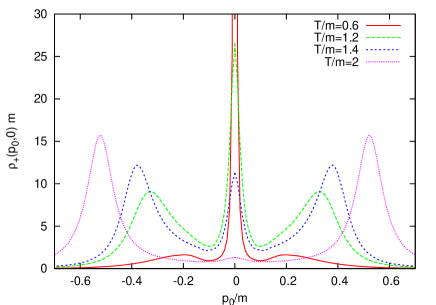
Figure 3: Temperature-dependence of the fermion spectral function $\rho_{+}m$ for $p=0,g^{2}=1$.

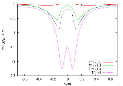
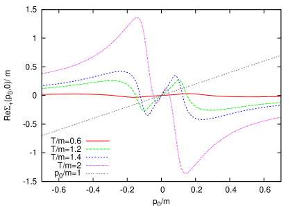
Figure 4: The fermion self-energy $\Sigma_{+}/m$ for $p=0,\,g^{2}=1$: the imaginary part (left panel) and the real part (right panel).

Figure 5: The kinetic processes by the Landau damping contained in the imaginary part of the fermion self-energy at one loop. (The corresponding inverse processes are not shown.) The solid line represents the fermion and the dashed one the on-shell boson with the energy $E_{p-k}=\sqrt{(\bm{p}-\bm{k})^{2}+m^{2}}$. The fermion with the energy $k$ is also on-shell.

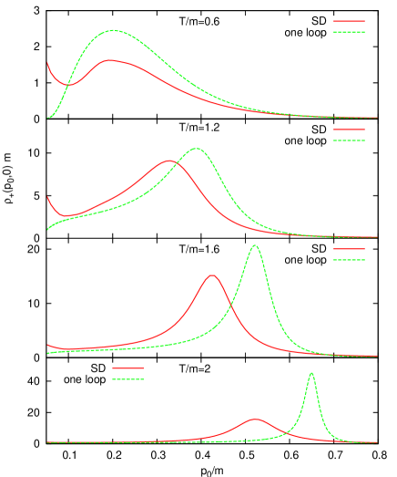
Figure 6: The spectral functions $\rho_{+}(p_{0},0)m$ for $g^{2}=1$ and $T/m=0.6,1.2,1.6,2$ from top to bottom.

In Fig. 2, we plot the fermion spectral function $\rho_{+}$ for various temperatures. At $T/m=0.6$, the peak position of the spectral function $\rho_{+}$ is almost on the light cone; $\rho_{+}$ has sharp quasiparticle peaks around $p_{0}=p$. At $T/m=0.8$, we see that the quasiparticle peaks are deformed near $p/m=0.2$ and that the peak position deviates from the light cone for $p/m\lesssim 0.2$. This deformation is more remarkable as $T$ is higher: At $T/m=1.0$ and $1.2$, the quasiparticle peaks start to split for $p/m\lesssim 0.2$, and there appear broad peaks both in the positive and negative energy regions around $p=0$. Therefore, we see a three-peak structure in the low-momentum region. At $T/m=1.6$, three peaks clearly separate from one another and the strength of the central peak becomes weaker than those of the peaks in both sides. At $T/m=2$, the central peak almost disappears and thus only two peaks remain in the low-momentum region. These two peaks correspond to the normal quasifermion and the antiplasmino seen in the spectrum in the HTL approximationKlimov:1981ka . The fact that these peaks survive for the strong coupling region is consistent with that in Refs.Harada:2007gg ; Peshier:1998dy .

In the same figure, as momentum is higher, the peak of the normal quasifermion becomes larger and sharper. This is because thermal effects get weaker and thus the spectrum should approach the free one up to the width due to quantum corrections as momentum is higher. The antiplasmino peak in turn rapidly suppresses as momentum is higher, which is consistent with the behavior of the HTL approximation where the residue of the (anti-)plasmino peak suppresses exponentially with momentum.

The above result resembles that obtained at the one-loop orderKitazawa:2006zi . Thus, higher order effects do not modify the qualitative peak-structure of the fermion spectrum at this coupling. There is, however, a quantitative difference for the central peak: While it is a $\delta$-function shape at the origin in the one-loop calculation, which can be shown analytically, it has a finite width in the present result. We plot $\rho_{+}$ at zero momentum in Fig. 3 from which we see that the width of the peak at the origin becomes broader and the peak height smaller as $T$ increases. It is noted that the behavior of the peak height is consistent with that in the one-loop calculation where the residue of the $\delta$-function peak becomes smaller as $T$ increases. The behavior of the peak height can be found from that of the self-energy at zero momentum shown in Fig. 4: We see that $|$Im$\Sigma_{+}(p_{0},\bm{0})|$ at the origin increases as $T$ increases, which means that the decay amplitude of the fermion increases with $T$. This is contrasted to the imaginary part of the self-energy at one loop which vanishes at the origin independently of $T$Kitazawa:2006zi . The reason of the vanishing at one loop is as follows. We can readily show that the fermion with the energy $-m<p_{0}<m$ and the zero momentum decays through the Landau damping shown in Fig. 5 at the one-loop order. It is noted that the boson and the out-going fermion are on-shell in this figure. Then, in the left process of Fig. 5, the boson momentum $k$ must be infinity for $p_{0}=0$ due to the energy-momentum conservation. Because this process and the inverse one give the statistical factor $n(\sqrt{k^{2}+m^{2}})+f(p_{0}+\sqrt{k^{2}+m^{2}})$ in the amplitude, these processes are forbidden for the infinite $k$. Likewise, in the right process of Fig. 5, the momentum of the in-coming fermion must be infinity for $p_{0}=0$ and then the statistical factor vanishes as in the left process. Therefore, we have always Im$\Sigma_{+}(0,\bm{0})=0$ at one loop. Because Re$\Sigma_{+}(p_{0},\bm{0})$ is an odd function by the charge conjugation invariance and thus vanishes at the origin at any order, the spectral function has a $\delta$-function shape at the origin. In the SD approach, on the other hand, higher loop effects do not forbid the decay of the fermion with $p_{0}=p=0$ and thus Im$\Sigma_{+}(0,\bm{0})$ can be finite, while Re$\Sigma_{+}(0,\bm{0})=0$ due to the property of the odd function as shown in the right panel of Fig. 4. This is the reason why there can exist a peak with a finite width at the origin in the SD approach. (In the right panel of Fig. 4, the line $p_{0}/m=1$ is also plotted. Crossing points between this line and Re$\Sigma_{+}$ give spectral peaks if Im$\Sigma_{+}/$Re$\Sigma_{+}$ is sufficiently small there.) We note, however, that it is nontrivial whether the three-peak structure appears in the SD approach because it would disappear if the value of Im$\Sigma_{+}(0,\bm{0})$ is quite large even for $T/m<2$. The result shown in Fig. 2 indicates that the three-peak structure is stable against higher order corrections at this coupling.

Next we examine the peaks in both sides which correspond to the normal quasifermion for $p_{0}>0$ and the anti-plasmino for $p_{0}<0$. In Fig. 6, we plot the spectral functions $\rho_{+}$ for $p_{0}>0$ and $p=0$ obtained from the SDE and the one-loop calculation. Because we have a relation $\rho_{+}(p_{0},\bm{0})=\rho_{+}(-p_{0},\bm{0})$, the anti-plasmino peak is also shown in this figure by replacing $p_{0}$ with $-p_{0}$ in the horizontal axis. At $T/m=0.6$ and $1.2$, the peak position and the width from the SDE are similar to those from the one-loop calculation. For higher $T$, the peak position and the width from the SDE are smaller and broader than those from the one loop, respectively. The broadening of the peak from the SDE could be understood from the fact that the probability of the boson emission and absorption from a fermion increases owing to multiple scatterings with bosons through the self-consistency conditionHarada:2007gg . The decrease of the peak position for higher $T$ due to nonperturbative effects is a new result, for which we do not have intuitive explanation in the present. As seen in the next subsection, this behavior of the decreasing peak position is also seen when the coupling $g$ becomes larger.

III.2 Coupling dependence

Figure 7: The fermion spectral functions $\rho_{+}m$ for $T/m=1$ and $g^{2}=0.4$ (left), 2 (middle), 4 (right). The figure is clipped at $\rho_{+}m=50$.

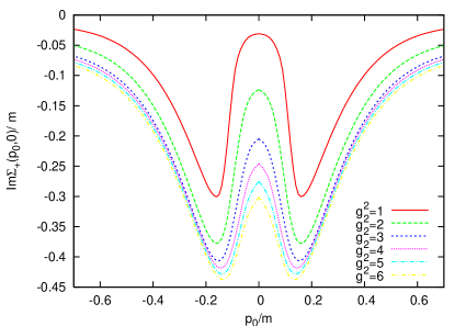
Figure 8: The imaginary part of the fermion self-energy $\Sigma_{+}/m$ for $p=0,\,T/m=1$.

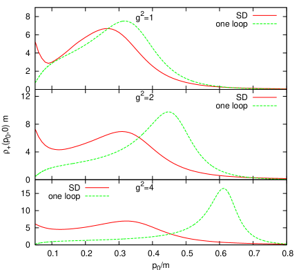
Figure 9: The spectral functions $\rho_{+}(p_{0},0)m$ for $T/m=1$ and $g^{2}=1,2,4$ from top to bottom.

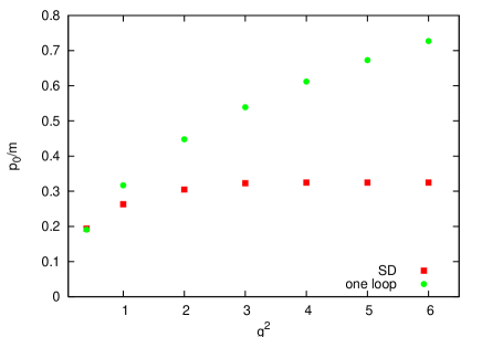
Figure 10: The peak position of the normal quasifermion for $p=0$ and $T/m=1$.

In this subsection, we study the coupling dependence of the fermion spectrum, focusing on the peak structure. In Fig. 7, we plot the fermion spectral function $\rho_{+}$ for $T/m=1$ and $g^{2}=0.4,2,4$. (For $T/m=1$ and $g^{2}=1$, see Fig. 2.) The fermion spectrum for $g^{2}=0.4$ is closer to the free spectrum than that for $g^{2}=1$ in Fig. 2, as it should be. For $g^{2}>1$, all the peaks at the low momentum region become broader and the height of the central peak falls rapidly. These properties are consistent with our previous work in which the fermion spectrum in a strong coupling gauge theory was investigated with the SDEHarada:2007gg : Because the SDE contains effects of multiple scatterings with bosons as mentioned in the previous subsection, the peak broadening for larger coupling could be understood from this point of view. The depression of the central peak is also understood from the multiple scattering effects: We plot the imaginary part of the fermion self-energy in Fig. 8. While the value at the origin is zero independently of the coupling at one loop as mentioned previously, its absolute value from the SDE gradually increases as the coupling increases. This means that higher order multiple scattering effects can bring about the decay of the fermion with $p_{0}=p=0$ and enhances as the coupling increases.

Next we consider nonperturbative effects of the fermion spectrum by comparing with the result of the one-loop calculation as shown in Fig 9. At $g^{2}=1$, the peak positions and the widths are close to each other. At $g^{2}=2,4$, the widths are broader than those at one loop, which is due to the multiple scattering effects as mentioned above. The peak positions are smaller than the one-loop results. More specifically, we plot the coupling dependence of the peak position at $p_{0}>0$ in Fig. 10. We see that the peak position from the SDE is smaller than that from the one loop and clearly saturates around $g^{2}=3$. This behavior is consistent with that obtained in Ref.Harada:2007gg . In the HTL approximation, the width of the corresponding peak vanishes and thus the peak position gives exactly the thermal mass which is proportional to $T$ and the coupling. Our results suggest that a simple extrapolation of the results by the perturbation theory to the strong coupling region is not valid for the thermal mass.

IV Concluding remarks and outlook

In this paper, we have investigated the fermion spectrum at finite temperature ($T$) in a chiral U(1)${}_{L}\times$ U(1)_R invariant linear sigma model employing coupled Schwinger-Dyson equations (SDE) for both fermion and boson with the ladder approximation. We formulate the SDE in the real time formalism and thus the spectrum in both the timelike and spacelike regions can be directly evaluated. To reduce the computation task, only the imaginary parts of the self-energies are evaluated with loop integrals, while the real parts are evaluated from the imaginary parts with the dispersion relation.

We have assumed the massless fermion and the massive boson and focused on the $T$ and coupling dependences of the fermion spectrum. The main reason is that it is pointed out from the one-loop evaluation in Yukawa models that the three-peak structure appears in the fermion spectrum at some $T$ and couplingKitazawa:2006zi ; Kitazawa:2007ep . The essential points of the existence of the three-peak structure found in Ref. Kitazawa:2006zi are the massiveness of the boson and the Landau damping at finite $T$. One of the remaining issues is whether such a structure is stable against higher order corrections, in particular, for the strong coupling region. Our present result supports the existence of the three-peak structure even in the strong coupling region, although the strength of the central peak rapidly suppresses owing to multiple scattering effects with bosons as the coupling increases. The quantitative difference between our result and the result from the one-loop calculation is that while the central peak at the origin is of the $\delta$-function shape at one loop, it has a finite width which becomes broader as the coupling and $T$ increase in the Schwinger-Dyson approach.

The present formalism can be readily applied to other models, such as gauge theories in the ladder approximation with the fixed gauge. Furthermore, because lattice QCD at high density is not realistic in the present, the extension to finite density systems is also important and, in fact, straightforward.

Because the soft bosonic modes are expected to arise dynamically near but above the critical temperature of the second order transition, it would be also interesting to extend this formalism in order to study effects of the phase transition and temperature-dependent bosonic masses. This should be possible in future study within the presented dynamical framework.

- (1) I. Arsene et al., Nucl. Phys. A 757, 1 (2005); B. B. Back et al., Nucl. Phys. A 757, 28 (2005); J. Adams et al., Nucl. Phys. A 757, 102 (2005); K. Adcox et al., Nucl. Phys. A 757, 184 (2005).
- (2) M. Asakawa and T. Hatsuda, Phys. Rev. Lett. 92, 012001 (2004); S. Datta, F. Karsch, P. Petreczky and I. Wetzorke, Phys. Rev. D 69, 094507 (2004); T. Umeda, K. Nomura and H. Matsufuru, Eur. Phys. J. C 39S1, 9 (2005); H. Iida, T. Doi, N. Ishii, H. Suganuma and K. Tsumura, Phys. Rev. D 74, 074502 (2006); A. Jakovac, P. Petreczky, K. Petrov and A. Velytsky, Phys. Rev. D 75, 014506 (2007); G. Aarts, C. Allton, M. B. Oktay, M. Peardon and J. I. Skullerud, Phys. Rev. D 76, 094513 (2007).
- (3) P. K. Kovtun, D. T. Son and A. O. Starinets, Phys. Rev. Lett. 94, 111601 (2005).
- (4) A. Schaefer and M. H. Thoma, Phys. Lett. B 451, 195 (1999); A. Peshier and M. H. Thoma, Phys. Rev. Lett. 84, 841 (2000).
- (5) M. Mannarelli and R. Rapp, Phys. Rev. C 72, 064905 (2005).
- (6) F. Karsch and M. Kitazawa, Phys. Lett. B 658, 45 (2007).
- (7) M. Harada, Y. Nemoto and S. Yoshimoto, Prog. Theor. Phys. 119, 117 (2008).
- (8) M. Kitazawa, T. Kunihiro and Y. Nemoto, Phys. Lett. B 633, 269 (2006).
- (9) T. Hatsuda and T. Kunihiro, Phys. Lett. B 145, 7 (1984); Phys. Rev. Lett. 55, 158 (1985).
- (10) M. Kitazawa, T. Kunihiro and Y. Nemoto, Prog. Theor. Phys. 117, 103 (2007).
- (11) M. Kitazawa, T. Kunihiro, K. Mitsutani and Y. Nemoto, Phys. Rev. D 77, 045034 (2008).
- (12) For a review of the SDE at finite , see, for example, C. D. Roberts and S. M. Schmidt, Prog. Part. Nucl. Phys. 45, S1 (2000).
- (13) A. Barducci, R. Casalbuoni, S. De Curtis, R. Gatto and G. Pettini, Phys. Rev. D 41, 1610 (1990); A. Barducci, R. Casalbuoni, G. Pettini and R. Gatto, Phys. Rev. D 49, 426 (1994).
- (14) K. I. Kondo and K. Yoshida, Int. J. Mod. Phys. A 10, 199 (1995).
- (15) Y. Taniguchi and Y. Yoshida, Phys. Rev. D 55, 2283 (1997).
- (16) D. Blaschke, C. D. Roberts and S. M. Schmidt, Phys. Lett. B 425, 232 (1998).
- (17) M. Harada and A. Shibata, Phys. Rev. D 59, 014010 (1998).
- (18) T. Ikeda, Prog. Theor. Phys. 107, 403 (2002).
- (19) S. Takagi, Prog. Theor. Phys. 109, 233 (2003).
- (20) H. Nakkagawa, H. Yokota and K. Yoshida, arXiv:0709.0323 [hep-ph].
- (21) See, for example, M. Le Bellac, Thermal Field Theory (Cambridge Unviersity Press, 1996).
- (22) S. Juchem, W. Cassing and C. Greiner, Phys. Rev. D 69, 025006 (2004).
- (23) H. A. Weldon, Phys. Rev. D 26, 2789 (1982).
- (24) V. V. Klimov, Sov. J. Nucl. Phys. 33, 934 (1981) [Yad. Fiz. 33, 1734 (1981)]; H. A. Weldon, Phys. Rev. D 40, 2410 (1989).
- (25) A. Peshier, K. Schertler and M. H. Thoma, Annals Phys. 266, 162 (1998).