KEK-CP-208
YITP-08-7
Two-flavor QCD simulation with exact chiral symmetry
Abstract
We perform numerical simulations of lattice QCD with two flavors of dynamical overlap quarks, which have exact chiral symmetry on the lattice. While this fermion discretization is computationally demanding, we demonstrate the feasibility to simulate reasonably large and fine lattices by a careful choice of the lattice action and algorithmic improvements. Our production runs are carried out on a lattice at a single lattice spacing around 0.12 fm. We explore the sea quark mass region down to , where is the physical strange quark mass, for a good control of the chiral extrapolation in future calculations of physical observables. We describe in detail our setup and algorithmic properties of the production simulations and present results for the static quark potential to fix the lattice scale and the locality of the overlap operator.
1 Introduction
Since lattice QCD emerged as a quantitative tool to study non-perturbative aspects of the strong interaction, enormous efforts have been made to calculate physical observables with controlled systematic uncertainties by large-scale simulations on increasingly finer and larger lattices. In particular, recent algorithmic improvements [1, 2, 3, 4, 5, 6, 7, 8] as well as development of computer technology enable us to approach the chiral regime of QCD [9, 10, 11, 12, 13, 14, 15, 16, 17] and to include all three light flavors of quarks dynamically [9, 10, 14, 15, 16, 18, 17].
The remaining crucial step towards the simulation of QCD is to preserve chiral symmetry on the lattice. Chiral perturbation theory (ChPT) based on this symmetry provides a theoretical guidance to the chiral extrapolation of physical observables to the quark mass in the real world. The explicit symmetry breaking in the conventional lattice actions for quarks distorts chiral behavior of the observables and introduces additional free parameters into ChPT [19, 20, 21, 22, 23, 24]. This makes the chiral extrapolation unstable unless one simulates a sufficiently wide region of the quark mass and the lattice spacing. Lattice operator mixing is another serious obstacle to precise calculations of hadronic matrix elements, such as the kaon parameter. We also note that massive Wilson-type Dirac operators are not protected from their (near-)zero modes due to the symmetry breaking. Studies on their spectrum [25, 26] suggest that it is safe to simulate fine and large lattices with this type of fermion discretization.
The five dimensional domain-wall formulation [27, 28, 29] restores chiral symmetry in the limit of infinitely large size in the fifth dimension, while it is times more costly with respect to the Wilson-type fermions. The RBC and UKQCD collaborations [14, 30] have been pursuing large-scale simulations employing – 20, with which the symmetry breaking is reduced to a level of a few MeV in terms of the additive quark mass renormalization.
There has been no large-scale simulations with negligible symmetry breaking, which is of course desirable and opens new possibility to study unexplored subjects such as the calculation of the chiral condensate and the pion mass splitting through the difference between vector and axial vector current correlators . The JLQCD collaboration has started such realistic simulations of QCD employing the overlap formulation [31, 32]. Its Dirac operator is
| (1) |
where is the quark mass and is the Hermitian Wilson-Dirac operator with a large negative mass . This formulation exactly111 Dirac operators satisfying the GW relation approximately have been proposed in Refs.[37, 38, 39] and have been employed in simulations in Refs.[40, 41]. satisfies the Ginsparg-Wilson (GW) relation [33]
| (2) |
and, hence, has exact chiral symmetry on the lattice [34, 35, 36]. Note that, in practical simulations, the lattice spacing should be sufficiently small to guarantee its locality.
The overlap fermions are however computationally more demanding than the domain-wall fermions. Simulations with dynamical overlap quarks have been limited to small and coarse lattices [42, 43, 44, 45, 46]. The main difficulty arises from the discontinuity of the overlap action Eq. (1) when an eigenvalue of changes its sign. This substantially impairs the efficiency of the commonly used Hybrid Monte Carlo (HMC) algorithm unless the time consuming reflection/refraction procedure [43] is implemented. In our dynamical overlap simulations, we avoid this overhead by suppressing zero modes of with a modification of the lattice action proposed in Ref.[47]. While this prevents us from sampling different topological sectors in a single simulation, the expectation values of physical observables in the QCD vacuum can be estimated by simulations in fixed topological sectors [48, 49].
In this article, we perform the first large-scale simulations with dynamical overlap quarks in two-flavor QCD. The above mentioned setup to fix the topology enables us to simulate a lattice spacing fm on a 2 fm box, which is comparable to those in recent studies with other discretizations. By implementing recent algorithmic improvements [3, 4, 5], the quark mass is reduced down to to control the chiral extrapolation of physical observables. As an example, we present our estimate of the lattice spacing through the Sommer scale [50] extrapolated to the chiral limit. The locality of the Dirac operator is a non-trivial issue for the GW fermions and is directly checked on the generated gauge ensembles. Status report of these production runs can be found in Refs.[16, 51, 52, 53, 54]. Simulations to study the -regime at a slightly fine lattice spacing have been already presented in Refs.[55, 56, 57, 58, 59].
This paper is organized as follows. We introduce our lattice action in Sec. 2. Section 3 is devoted to a description of our simulation algorithm. In Sec. 4, we present our choice of simulation parameters and discuss algorithmic aspects of our production runs in detail. We present results for the static quark potential and the locality of the overlap operator in Secs. 5 and 6, respectively. Our conclusions are given in Sec. 7.
2 Lattice action
We employ the overlap quark action Eq. (1) which can be rewritten in terms of the massless Dirac operator as
| (3) | |||||
| (4) |
The parameter should be adjusted so that the overlap operator has good locality properties. We set , which was also employed in a previous simulation in quenched QCD around our target lattice spacing [60]. The locality with our simulation setup is checked on generated gauge ensembles in Sec.4.
A major problem with the unsmeared Wilson kernel is the appearance of its (near-)zero modes on relatively coarse lattices. This makes simulations costly and possibly spoils the locality of . One way to reduce the localized (near-)zero modes is the use of improved gauge actions leading to smooth gauge configurations [61]. In our simulations, we employ the Iwasaki gauge action [62]
| (5) |
where , and and are and Wilson loops in the plane. Their weights are and . In our preparatory study in quenched QCD [54], we find that (near-)zero modes are remarkably reduced and the overlap operator shows better locality properties by switching the standard plaquette gauge action to this improved action.
We however need to rule out the appearance of exact zero modes in order to avoid the time-consuming reflection/refraction step [43]. To this end, we introduce two copies of unphysical Wilson fermions with the large negative mass [47, 63, 64] and two copies of twisted mass ghosts [47] leading to the following auxiliary fermionic determinant
| (6) |
The numerator suppresses the zero modes during continuous evolutions of the gauge field such as HMC, whereas effects of high modes of are cancelled by the denominator. The twisted mass parameter is tuned to compromise between the suppression of the zero modes and reduction of the shift due to the unphysical fermions. It should be noted that these unphysical fields have a mass of and hence they do not change the continuum limit of the theory. Their effects can be simply considered as a modification of the gauge action by .
The auxiliary determinant fixes the net topological charge during the HMC update. We note however that local topological fluctuations are not suppressed in this setup: actually the topological susceptibility is calculable in a topological sector as demonstrated in Ref.[65]. The correction due to the fixed global topology can be considered as a finite size effect, which is suppressed by the inverse space-time volume [48, 49]. In addition, the expectation values of physical observables in the QCD vacuum can be estimated by studying their dependence from simulations in fixed topological sectors [48, 49]. The conventional setup, on the other hand, can sample different topological sectors through lattice dislocations, i.e. discontinuities of a gauge configuration. They occur by short distance statistical fluctuations and also by the appearance (or disappearance) of more physical topological objects, such as instantons, of order of lattice spacing. Both of these effects yielding the topological tunneling are increasingly more suppressed as the continuum limit is approached. Our setup to fix the topology (or modified algorithms such as in Refs.[66, 67]) is an interesting alternative in future simulations near the continuum limit. It is also noteworthy that our setup provides a framework useful to study the -regime of QCD, as demonstrated in Refs.[57, 58, 59].
3 Simulation algorithm
3.1 Multiplication of overlap operator
A central building block in our HMC program is the multiplication of the overlap operator to a given quark field vector . We evaluate the sign function in with the low mode preconditioning. Namely, we introduce a threshold in the spectrum of and normalized eigenmodes with their eigenvalues are determined by the implicitly restarted Lanczos algorithm. We denote the number of the low modes thus extracted by in the following. These modes are projected out in the multiplication of
| (7) |
where is the projection operator on to the eigenspace spanned by . We also determine the largest eigenvalue . The contribution of higher modes is then estimated by a minmax rational approximation
| (8) |
with the Zolotarev coefficients , for the range [68, 69]. The multiple inversions for can be carried out simultaneously by the multi-shift conjugate gradient (CG) algorithm [70, 71]. We keep and constant while varies as a result of fixing . This together with small statistical fluctuation of makes the accuracy and the computational cost in the evaluation of stable.
3.2 Overlap solver
We need to solve the linear equation
| (9) |
for a given source vector in preparations of pseudo-fermions and calculations of the Molecular Dynamics (MD) forces in HMC. In the early stage of our simulation, we evaluate by the nested four dimensional (4D) CG algorithm, which consists of multi-shift CG for as the inner solver and CG for normal equations (CGNE) to evaluate as the outer solver. As the outer solver proceeds, the computational cost of the inner solver can be substantially reduced by adjusting its stopping condition
| (10) |
where is the iteration count for the outer solver [72, 73]. We employ the relaxed stopping condition outlined in Ref.[73]. This is based on the idea that, as the outer solver proceeds, the correction to the solution vector becomes smaller and we do not have to evaluate with too much accuracy. Its implementation depends on the outer solver algorithm and, for CG(NE), the condition is loosened as
| (11) |
where is the residual for the outer solver at -th iteration. It was observed on small lattices [73] that this relaxation leads to roughly a factor of 2 reduction in the computational cost.
For a further improvement in the solver performance, we later switch to the five dimensional (5D) solver proposed in Refs. [74, 75, 76]. In the case of for instance, we consider the following 5D matrix to solve Eq. (9)
| (19) |
where and are the coefficients in the Zolotarev approximation Eq. (8) and . The Schur decomposition
| (26) |
contains the Hermitian overlap operator as the Schur compliment
| (27) |
Its inverse can be evaluated by solving the 5D equation
| (32) |
We observe that the convergence of this solver can be improved by a preconditioning based on the 5D structure , where is obtained from by setting all gauge links to zero. Note that is local, uniform in space-time, and easy to invert through its LU decomposition and forward/backward substitutions. This is naturally incorporated into the even-odd preconditioning [76]
| (33) |
since where the subscripts “e” and “o” represent even and odd sites. It turns out in Sec. 4 that this preconditioned solver is roughly a factor of 3 faster than the relaxed 4D solver.
3.3 HMC
In our implementation of HMC, we employ a combination of the Hasenbusch preconditioning [4, 5] and the multiple time scale integration for MD [3], which has been shown to be very effective in simulations with Wilson-type fermions [77, 78]. In our HMC program with the 4D overlap solver, which is referred to as “HMC-4D” in the following, the fermionic determinant is expressed as
| (34) |
where is the mass of the Hasenbusch preconditioner. Two determinants as well as from the extra-Wilson fermions are evaluated by introducing three pseudo-fermions , , : namely
| (35) | |||||
| (36) |
and
| (37) | |||
| (38) |
where is the Dirac operator for the twisted mass Wilson fermions.
The expression of the force associated with the overlap pseudo-fermion is already available in Refs. [42, 43, 45, 46]. Here, we explicitly write down only the simplest one from
| (39) |
where and the derivative of the sign function is given by
| (40) |
Hence, we need to evaluate by the 4D relaxed CGNE and also have to invoke the multi-shift CG to calculate . The forces and from the overlap pseudo-fermion actions and are much more expensive to evaluate than from and the gauge force .
The use of the multiple time scale integration is therefore crucial to reduce the computational cost of the MD evolution. We employ the following three nested loops
| (41) | |||||
| (42) | |||||
| (43) |
where evolves the gauge field by the MD step size , and updates the conjugate momentum with the MD force (). We put together with in the inner-most loop, otherwise the suppression of the (near-)zero modes of fails by a mismatch between the updated gauge configuration and . The integration scheme can be largely accelerated by an appropriate choice of positive integers and when the magnitude of the forces are well separated from each other. This point is one of the central issues in the next section.
The reflection/refraction step is designed to deal with the discontinuity in the Hamiltonian along the MD evolution of the gauge field, and hence has to be included into in the inner-most loop. This step requires a significant computational cost to accurately locate at which point of the MD evolution the sign of an eigenvalue of changes. In our simple implementation, moreover, it involves two inversions of the overlap operator to evaluate the Hamiltonian just before and after the change of the sign222 Improved implementations of the reflection/refraction step are proposed in Refs.[79, 80]. . This step therefore could lead to a considerable slow down of simulations. The determinant enables us to avoid this serious overhead.
In HMC with the 5D solver, which we call “HMC-5D” in the following, we have to modify the implementation of HMC due to the lack of the low mode preconditioning. The coefficients and for the 5D solver are determined with an appropriate choice of and , which are kept fixed during our simulation. This could lead to a sizable error in , when has eigenvalues smaller than . In order to keep the accuracy of comparable to that in HMC-4D, the fermionic determinant is modified as
| (44) |
where represent the less accurate overlap operator without the low mode preconditioning. The first two determinants are dealt with by the usual HMC steps, whereas the last factor is taken into account by the noisy Metropolis test [81]. The probability is evaluated as
| (45) |
where is a random Gaussian noise vector and is on the final (initial) gauge configuration. Therefore, this step needs to invert both of and and spends a significant fraction of the total CPU time.
Another difference from HMC-4D is that is evaluated by invoking CGNE twice for Eq. (33), since no 5D representation is available for . It turns out that, however, CGNE is effective in inverting the preconditioned 5D matrix in Eq. (33) and switching CGNE to MINRES does not lead to a substantial reduction in the computational cost.
3.4 Machine
Our numerical simulations are carried out on the supercomputer system at KEK. This is a combination of 16 nodes of Hitachi SR11000 and 10 racks of IBM Blue Gene/L, whose peak speeds are about 2.15 and 57.3 TFLOPS, respectively. Our measurement of the static quark potential is inexpensive and is carried out on the SR11000 computer. The configuration generation with the above mentioned HMC algorithm is computationally intensive and is carried out on Blue Gene/L. To increase the sustained speed as much as possible, we employ an assembler code developed by the IBM Japan for the multiplication of . This code makes the best use of the so-called double FPU instructions, which process complex-arithmetic operations in double precision effectively using two arithmetic pipelines. It also has a good scalability with respect to the number of computing nodes by using a low-level interface for inter-node communications. We find that this assembler code is roughly a factor of 3 faster than our naive Fortran code.
4 Production Run
4.1 Simulation parameters
We simulate QCD with two flavors of degenerate up and down quarks employing the lattice action introduced in Sec. 2. The twisted mass for the auxiliary determinant is set to from our studies in quenched QCD [47, 54]. Numerical simulations are carried out on a lattice at a single value of , which is expected to correspond to our target lattice spacing 0.125 fm. The box size should be around 2 fm. In the trivial topological sector, we simulate six sea quark masses listed in Tables 1 and 2. From our analysis of the meson spectrum [82], this choice covers a range from down to in physical units. The statistics are 10,000 HMC trajectories at each quark mass with the unit trajectory length set to 0.5. At which roughly corresponds to , we also accumulate 5,000 trajectories in the non-trivial topological sectors with and . The initial gauge configuration for these runs is prepared as in Ref. [83]. The generated gauge configurations are stored on disks every 10 trajectories for future measurements of physical observables. These parameters are summarized in Tables 1 and 2.
| HMC traj. | time[min] | |||||||||
|---|---|---|---|---|---|---|---|---|---|---|
| 0.015 | 0 | 10 | 0.108 | 0.2 | 9 | 4 | 5 | 2800 | 0.875(7) | 50 |
| 0.025 | 0 | 10 | 0.108 | 0.2 | 8 | 4 | 5 | 5200 | 0.900(3) | 41 |
| 0.035 | 0 | 10 | 0.108 | 0.4 | 6 | 5 | 6 | 4600 | 0.739(7) | 28 |
| 0.050 | 0 | 10 | 0.108 | 0.4 | 6 | 5 | 6 | 4800 | 0.781(5) | 23 |
| 0.070 | 0 | 10 | 0.108 | 0.4 | 5 | 5 | 6 | 4500 | 0.818(7) | 20 |
| 0.100 | 0 | 10 | 0.108 | 0.4 | 5 | 5 | 6 | 4600 | 0.852(5) | 17 |
| 0.050 | 10 | 0.108 | 0.4 | 6 | 5 | 6 | 1100 | 0.762(13) | 24 |
| HMC traj. | time[min] | |||||||||
| 0.015 | 0 | 10 | 0.108 | 0.2 | 13 | 6 | 8 | 7200 | 0.686(6) | 26 |
| 0.025 | 0 | 10 | 0.108 | 0.2 | 10 | 6 | 8 | 4800 | 0.816(5) | 22 |
| 0.035 | 0 | 10 | 0.108 | 0.4 | 10 | 6 | 8 | 5400 | 0.875(5) | 19 |
| 0.050 | 0 | 10 | 0.108 | 0.4 | 9 | 6 | 8 | 5200 | 0.879(5) | 15 |
| 0.070 | 0 | 10 | 0.108 | 0.4 | 8 | 6 | 8 | 5500 | 0.917(4) | 13 |
| 0.100 | 0 | 10 | 0.108 | 0.4 | 7 | 6 | 8 | 5400 | 0.926(3) | 11 |
| 0.050 | 10 | 0.108 | 0.4 | 9 | 6 | 8 | 3900 | 0.882(5) | 15 | |
| 0.050 | 10 | 0.108 | 0.4 | 9 | 6 | 8 | 5000 | 0.872(5) | 15 |
| HMC traj. | time[min] | |||||||||||
|---|---|---|---|---|---|---|---|---|---|---|---|---|
| 2.45 | 0.0 | 0.090 | – | 12 | 0.096 | 0.4 | 6 | 5 | 6 | 300 | 0.78 | 46 |
| 2.35 | 0.2 | 0.110 | 0 | 10 | 0.144 | 0.4 | 5 | 5 | 6 | 1200 | 0.87 | 12 |
In the course of our calibration of the lattice spacing, we investigate the impact of the auxiliary determinant on the computational cost at a slightly finner lattice spacing at . A single quark mass around is simulated without the determinant (namely, ) but with the reflection/refraction procedure. This run can be compared to one of our simulations with at a similar lattice spacing, which has been reported in Ref.[58]. We summarize parameters of these runs in Table 3.
4.2 Autocorrelation
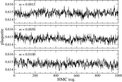
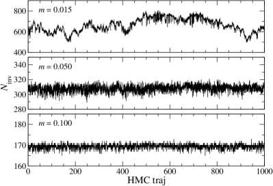
We first discuss the autocorrelation in our simulations to fix the bin size used in the jackknife analysis in the subsequent sections. In Fig. 1, we plot the time history of the plaquette and the number of iterations to invert in the simulations with HMC-4D. It is observed that shows longer and larger fluctuations as decreases, while such a tendency is not clear in the plaquette.
A conventional measure of the autocorrelation of an observable is the integrated autocorrelation time defined by
| (46) |
through the normalized autocorrelation function
| (47) |
where the Monte Carlo average (over ) is explicitly indicated by the bracket . Practically, the sum in Eq. (46) has to be truncated at a certain value of . In this analysis, we employ the condition adopted in Ref.[7]: namely, is set to the minimum value of satisfying
| (48) |
where is the standard deviation of estimated by the Madras-Sokal formula [84, 85].
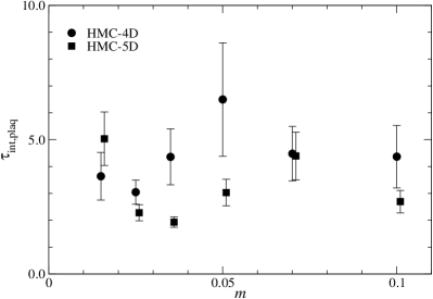
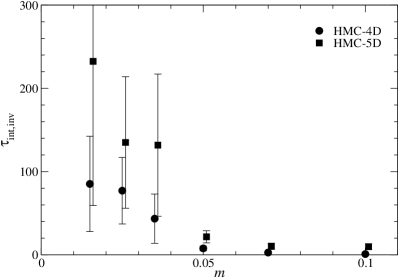
In Fig.2, we plot for the plaquette and for as a function of . It turns out that is not large (about 5 trajectories) and has small dependence, probably because it is a local quantity. On the other hand, is expected to be sensitive to the low modes of , and in fact increases to trajectories at small quark masses . While these observations are consistent with Fig. 1, it is clear that our statistics are not sufficiently large to estimate accurately at small .
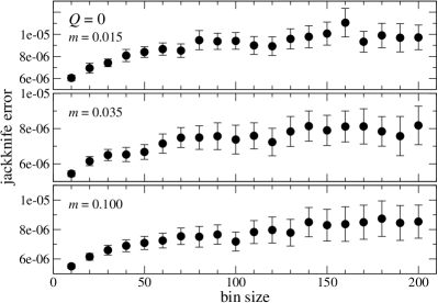
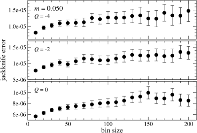
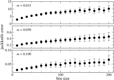
Therefore, we also check the bin size dependence of the jackknife error in Fig. 3, where two data of the plaquette obtained with HMC-4D and 5D are combined. Roughly speaking, the jackknife error becomes stable when the bin size is – 200 trajectories irrespective to the choice of and . At similar bin sizes, the jackknife error of also becomes stable as shown in Fig. 4. From these observations, we employ the bin size of 200 trajectories throughout this article, unless otherwise stated. Although only a limited number of bins are available to analyze algorithm-dependent quantities, such as , in simulations with HMC-4D at and , it turns out that decreasing the bin size leads to an even smaller statistical error for such quantities. For a reference, the plaquette averaged over our full statistics and its jackknife errors are summarized in Tables 4 and 5.
| 0.015 | 0.025 | 0.035 | 0.050 | 0.070 | 0.100 | |
|---|---|---|---|---|---|---|
| plaq. | 0.614789(10) | 0.614777(9) | 0.614764(8) | 0.614718(9) | 0.614709(10) | 0.614667(9) |
| (0.050,-2) | (0.050,-4) | |
|---|---|---|
| plaq. | 0.614762(13) | 0.614704(15) |
4.3 Spectral density of and
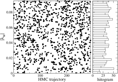
In Fig. 5, we compare the low-lying spectrum of in our test runs listed in Table 3. Without the auxiliary determinant , has an almost uniform density in the investigated region . This causes the reflection (refraction) occurring roughly 130 (14) times per 100 trajectories at our lattice spacing which is only slightly coarser than those in recent simulations with Wilson-type actions. In contrast, near-zero modes are remarkably suppressed by the determinant. We can safely turn off the reflection/refraction without a serious loss in the acceptance rate and observe about a factor of 4 reduction in CPU time as in Table 3.
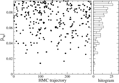
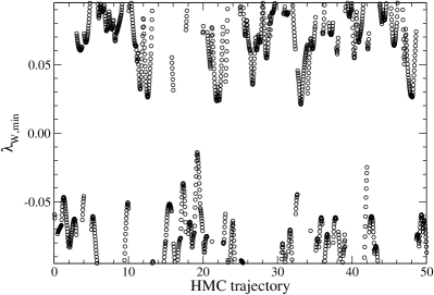
In Fig. 6, we plot the eigenvalue distribution in our production simulations at several quark masses. Near-zero modes are successfully suppressed also in these high statistics runs, and resulting distribution has small dependence, as it should. Figure 7 shows the MD evolution of the lowest eigenvalue . We observe that approaching to is eventually bounced back by the repulsive force from the potential barrier generated by the determinant.
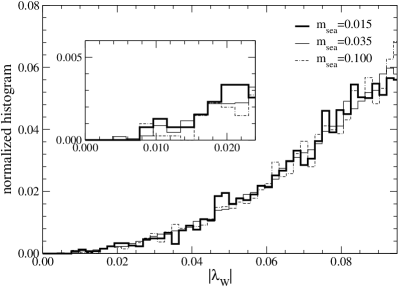
The suppression of near-zero modes enables us to take a relatively large value for the threshold and thus small in the multiplication of . We set at all values of based on the small dependence of the low mode distribution in Fig. 6. There are only a few eigenvalues below this threshold, and hence it does not take too much time to determine such low-lying modes with a strict condition
| (49) |
for the low-mode preconditioning Eq. (7). We set with which the accuracy of the Zolotarev approximation Eq. (8) is typically .
In simulations with HMC-5D, we consider saving the CPU time by loosening the approximation of for and in Eq. (44), since the noisy Metropolis test guarantees that gauge configurations are generated with the fermionic determinant of the accurate overlap operator . We set for the Hasenbusch preconditioner . Since the error of the rational approximation scales as , this is less accurate compared to with for HMC-4D. While Fig. 6 shows that there appear a non-negligible number of eigenmodes below , HMC-5D achieves the reasonable acceptance rate listed in Table 2. This suggests that the error due to the rough approximation in ’s as well as that due to the lack of the low mode preconditioning are stochastically cancelled (in part) between and in the MD integration. We set for , since relatively large leads to a substantially poor acceptance rate for the noisy Metropolis test.
4.4 and overlap solvers
Our HMC programs involve various stopping conditions. We need to specify conditions for the 4D overlap solver
| (50) |
and those for the 5D solver
| (51) |
where the subscript is “” or “” representing the condition for the calculation of the MD force or the Hamiltonian. Note that is the condition fulfilled by the 5D preconditioned solution vector . Our numerical test suggests that should be stricter than by one or two orders of magnitude so that the accuracy of the 4D piece in is comparable to that by the 4D solver with .
The stopping condition for the multi-shift CG inside the 4D overlap solver is automatically determined by Eq. (11) except for the initial residual . An appropriately strict value is employed to calculate with the given initial guess . Therefore, we only need to specify conditions for multiplications of and calculations of by Eq. (40)
| (52) |
with or “’. Here the condition in HMC-4D (5D) is represented by the subscript (“5D”). In our production run, we employ a rather strict condition for calculations of the Hamiltonian in order to carry out the Metropolis tests accurately.
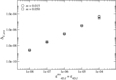
The choice of and is crucial to save the computational cost but should be strict enough to make our HMC reversible. The conventional measures of the reversibility violation in the gauge links and the Hamiltonian are
| (53) | |||||
| (54) |
where and are color indices and note that our unit trajectory length is 0.5. We pick up ten gauge configurations separated by 200 trajectories, and calculate and by updating them by one trajectory and then evolving back with the reversed momenta. Figure 8 shows these measures in HMC-4D, for which we set for simplicity. We observe a monotonous decrease in both measures and small dependence of their size. By employing
| (55) |
at all quark masses, the reversibility in our simulations is preserved at a level of and , which are comparable to those in previous large-scale simulations with the Wilson-type actions [86, 87, 88]. A similar study for HMC-5D leads us to set
| (56) |
in order to maintain the reversibility at the same level to HMC-4D.
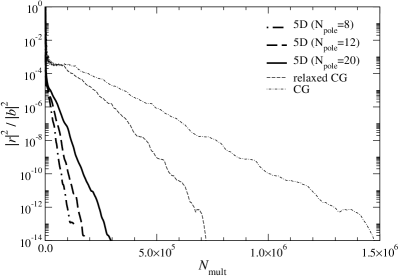
In Fig. 9, we compare the convergence of the 4D and 5D solvers by plotting the normalized residual as a function of the number of the multiplication . We take and turn off the low mode preconditioning by setting for a fair comparison between the 4D and 5D algorithms. The relaxed condition Eq. (11) works well on our 2 fm box and achieves about a factor of 2 speed up compared to the standard CG. The 5D solver is even faster by about a factor of 3 mainly due to the preconditioning of Eq. (33). We observe an acceleration of similar magnitude also at other quark masses.
It is an interesting issue how the computational cost scales as a function of . The iteration count of our overlap solver depends on through eigenvalues of . For simplicity, we use the following approximation for low-lying eigenvalues
| (57) |
where is the -th eigenvalue of the massless Dirac operator projected to the imaginary axis
| (58) |
and we ignore the small correction factor in Eq. (3). The dependence of in HMC-4D is then expected to be
| (59) |
with the power for CGNE.
| algorithm | ||
|---|---|---|
| HMC-4D | 22.86(9) | 0.869(1) |
| HMC-5D | 159(8) | 0.64(2) |
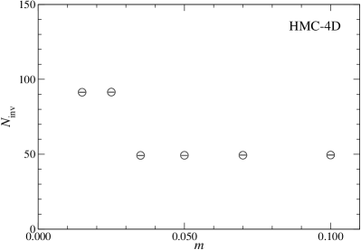
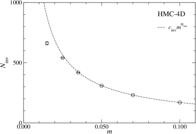
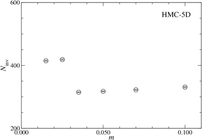
The mass parameter in Eq. (59) should be for the Hasenbusch preconditioner . Since we take large values for , is governed by and has small dependence as shown in Fig. 10. On the other hand, to invert increases monotonously as decreases. Data at four heaviest quark masses are reasonably described by the scaling law Eq. (59) with neglected
| (60) |
Fit parameters are listed in Table 6. We note that the power is close to its maximum value .
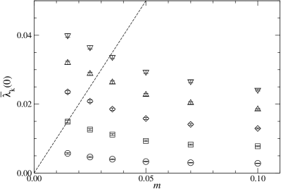
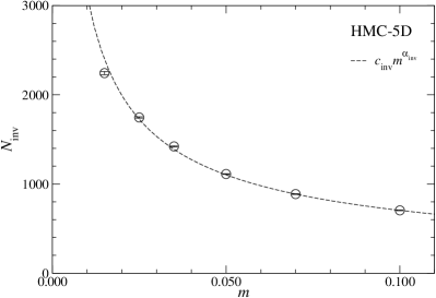
Our data of at however clearly deviate from this fit. This can be considered as a manifestation of finite size effects as we approach the -regime by decreasing with the fixed spatial extent [57, 58]. Figure 11 actually shows that the magnitude of in units of rapidly increases toward smaller . Namely, at heavy quark masses , for CGNE has dense low-lying eigenvalues near and, hence, is a good parameter to characterize its condition number. On the other hand, becomes sparse and deviates from as decreases. It is likely that this rapid change in the low mode distribution distorts the dependence of from the simple scaling Eq. (60).
4.5 Properties of HMC
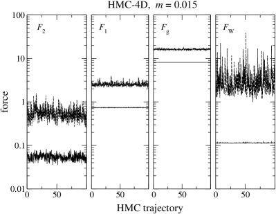
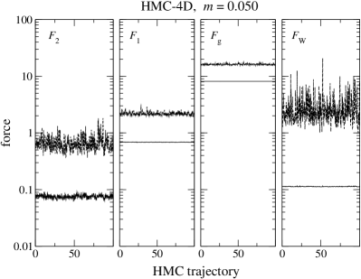
The parameters for the Hasenbusch preconditioning, Eqs. (34) and (44), and the multiple time scale MD integration, Eqs. (41) – (43), are listed in Tables 1 – 2. The gauge force is known to be generally larger than the fermionic force(s). Only needs a non-trivial tuning to make a hierarchic structure among the MD forces , and . As discussed in Refs.[5, 78], should be decreased for smaller to avoid a too large condition number for the preconditioned Dirac operator . This is why is set to a smaller value at than others. While we have not done further fine tuning of , Figs. 13 and 14 show that the forces , and are well separated from each other with our choice of . This enables us to use the ratios of the step sizes, namely and , around 4 – 8, which considerably reduce the computational cost of the MD integration with the acceptance rate kept in a reasonably high range .
The same figures show that from the extra-Wilson fermions exhibits large statistical fluctuations. It becomes as large as probably due to the appearance of small eigenvalues of . This is another reason why we update in the inner-most loop in Eq. (43), in addition to its consistency with the updated gauge field described in Sec. 3.

| HMC-4D | HMC-5D | ||||
|---|---|---|---|---|---|
| 0.015 | 0 | 0.0603(72) | 0.9957(64) | 4618(4617) | 0.998(14) |
| 0.025 | 0 | 14(14) | 0.9954(32) | 0.1142(52) | 0.9997(59) |
| 0.035 | 0 | 0.2224(86) | 1.016(11) | 0.068(15) | 0.9964(42) |
| 0.050 | 0 | 0.1846(84) | 1.0008(83) | 0.0519(39) | 0.9982(45) |
| 0.070 | 0 | 0.198(99) | 0.9989(52) | 0.0260(29) | 0.9950(24) |
| 0.100 | 0 | 0.0692(33) | 0.9963(34) | 0.0207(33) | 0.9989(30) |
| 0.050 | -2 | 0.37(16) | 0.978(15) | 0.0432(80) | 1.0082(61) |
| 0.050 | -4 | – | – | 0.0601(55) | 0.9934(52) |
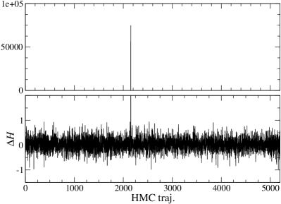
We denote the change in the Hamiltonian due to the discretized MD integration by and its average is summarized in Table 7. The area-preserving property of MD leads to the following (in)equality
| (61) |
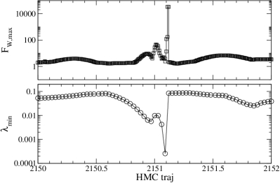
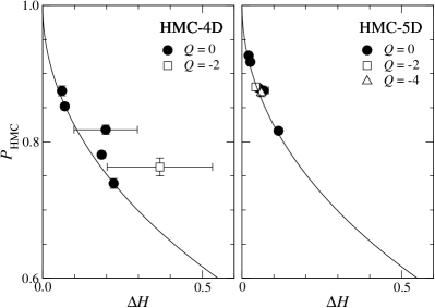
where we explicitly indicate the value averaged over HMC updating by the bracket . The inequality predicts that averaged is positive and this is the case in our simulations. Two of them are however dominated by huge spikes shown in Fig. 15. Similar spikes have been observed also in previous simulations with Wilson-type fermions [89], and they may be attributed to instability of HMC with a large MD step size [90]. The spikes in our simulations have rather simple origin as shown in Fig. 16: can develop a very small lowest eigenvalue leading to a spike in and hence in . This is why we take a larger value for in HMC-5D to be more robust against the spikes with a smaller MD step size for the calculation of . Thanks to the determinant , however, the number of such huge spikes is not large even in HMC-4D, at most a few per 10,000 trajectories. As a result, the equality Eq. (61) is fulfilled within 2 % accuracy without introducing the replay trick [6, 91]. We also note that dependence of is consistent with the expected form of the complementary error function
| (62) |
as plotted in Fig. 17.
4.6 Simulation cost
On a half rack of Blue Gene/L, the assembler code for the multiplication of achieves roughly 28 % efficiency of the peak performance when all the data are in the L3 cache. The sustained speed averaged over all HMC steps is about 15 % indicating significant overheads due to a limited bandwidth to the off-chip memory, and to linear computations with quark vectors in the low mode preconditioning and so on.
In Table 8, we summarize the number of multiplications per trajectory, which serves as a machine independent measure of the simulation cost. This is compared with at each HMC step in Fig. 18. As expected, calculations of the overlap forces and spend a large part of the total CPU time especially at small quark masses . Note also that the costs to calculate the two forces are of the same order: in other words, they are reasonably balanced with our choice of and . While is calculated in the inner-most loop of our MD integration, its computational cost turns out to be negligible in HMC-4D, and is not large even in HMC-5D, where the overlap solver is accelerated by the 5D algorithm.
| 0 | -2 | -4 | ||||||
|---|---|---|---|---|---|---|---|---|
| 0.015 | 0.025 | 0.035 | 0.050 | 0.070 | 0.100 | 0.050 | 0.050 | |
| HMC-4D | 11.9(1) | 7.6(4) | 5.0(2) | 4.5(2) | 3.4(1) | 3.1(1) | 5.08(2) | – |
| HMC-5D | 6.53(4) | 5.10(2) | 4.41(2) | 3.62(1) | 2.98(1) | 2.44(1) | 3.61(2) | 3.65(1) |
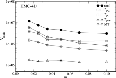
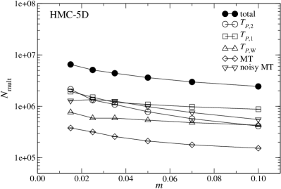
In simulations with HMC-5D, the noisy Metropolis test also needs a substantial fraction of the total time. This is because it has to invoke the 4D solver with the strict stopping condition to calculate the probability Eq. (45) accurately, whereas other HMC steps are implemented with the much faster 5D solver. We note that this step is removed in our latest -flavor simulations by incorporating the low-mode preconditioning into the 5D solver [16, 15].
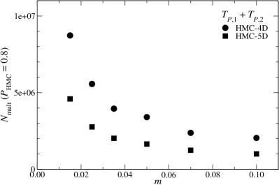
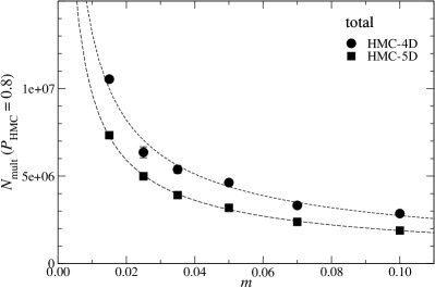
Figure 19 shows a comparison between HMC-4D and HMC-5D in total and that for and . To take the difference in into account, in this figure is corrected by a factor , where is the step size corresponding to estimated by assuming Eq. (62) and . Due to the rough approximation and the lack of the low-mode preconditioning for in , have to be decreased by roughly 50% when the algorithm is switched from HMC-4D to HMC-5D with kept fixed. Even with this overhead, we observe about factor of 2 reduction in for and . The noisy Metropolis test reduces the net gain to roughly 50% at all the simulated quark masses. We note in passing that the CPU time summarized in Tables 1 and 2 shows slightly better acceleration than in at . This is because the low-mode preconditioning leading to the overhead mentioned at the beginning of this subsection is switched off in the 5D solver.
| algorithm | ||
|---|---|---|
| HMC-4D | 0.57(3) | 0.68(2) |
| HMC-5D | 0.368(3) | 0.710(3) |
For future reference, we fit dependence of the corrected into a simple power law
| (63) |
Fit parameters are summarized in Table 9. While data at small are subject to the finite size effects as discussed in Sec. 4.4, the fit parameters do not change significantly if we discard the data at from the fit. Note that this is the cost per trajectory and the dependence of the autocorrelation, which is not clear with our statistics, is not taken into account. Thanks to the improved algorithms, has a much milder dependence than , which was employed to estimate the simulation cost with the standard HMC in Ref.[92].
In Table 8, we also list in the non-trivial topological sectors. At least at the simulated quark mass , we have not observed a substantial dependence of .
5 static quark potential
We calculate the static quark potential to fix the lattice spacing through the Sommer scale [50]. The temporal Wilson loops are measured up to and with the spatial Wilson line parallel to one of the following six directions
| (64) |
Gauge configurations separated by 10 HMC trajectories are smeared twenty times using a method proposed in Ref.[93], and we measure every four smearing steps. The computational cost of this measurement is not large: it takes about 2 minutes per configuration on a single node of SR11000 with the sustained speed of 30%.
We determine the static potential from the correlated fit
| (65) |
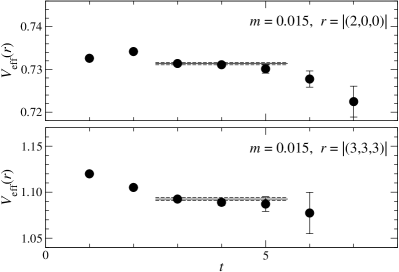
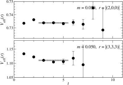
at the number of the smearing steps which gives the maximum value of the overlap to the ground state . The fit range is set to by inspecting -dependence of the effective potential
| (66) |
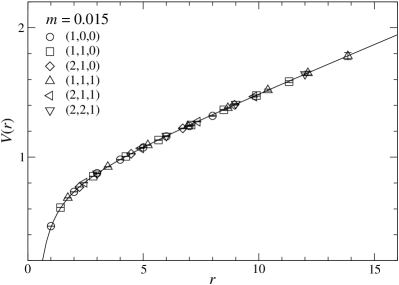
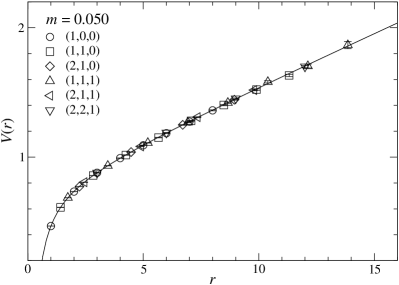
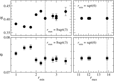
Examples of are shown in Fig. 20, and is plotted as a function of in Fig. 21.
| 2.30 | 0.015 | 0 | 0.786(3)(15) | 0.403(5)(28) | 0.0740(6)(26) | 4.103(14)(51) |
|---|---|---|---|---|---|---|
| 2.30 | 0.025 | 0 | 0.776(4)(21) | 0.389(5)(36) | 0.0763(7)(37) | 4.064(13)(59) |
| 2.30 | 0.035 | 0 | 0.769(4)(22) | 0.381(5)(38) | 0.0780(6)(34) | 4.032(10)(49) |
| 2.30 | 0.050 | 0 | 0.760(3)(16) | 0.375(5)(30) | 0.0812(7)(26) | 3.963(11)(42) |
| 2.30 | 0.070 | 0 | 0.756(4)(25) | 0.373(6)(42) | 0.0832(7)(40) | 3.917(11)(40) |
| 2.30 | 0.100 | 0 | 0.749(4)(18) | 0.368(5)(30) | 0.0864(7)(30) | 3.852(10)(35) |
| 2.30 | 0.050 | -2 | 0.759(7)(24) | 0.370(11)(44) | 0.0803(12)(34) | 3.993(16)(29) |
| 2.30 | 0.050 | -4 | 0.758(6)(20) | 0.368(10)(36) | 0.0811(12)(29) | 3.976(19)(36) |
We do not observe any clear sign of the string breaking even at our smallest quark mass possibly due to small overlap of the spatial Wilson line to the two static-light meson state. We therefore fit to the conventional form with the perturbative Coulomb and the linear confinement terms
| (67) |
The fit range is set to at all quark masses from the stability of and against the choice of the fit range shown in Fig. 22. Fit results are summarized in Table 10. Systematic errors due to the choice of the fit ranges are estimated from the (maximum) change in the fit parameters by shifting to or varying and in ranges and . These are added in quadrature in Table 10. The fit curves are shown in Fig. 21.
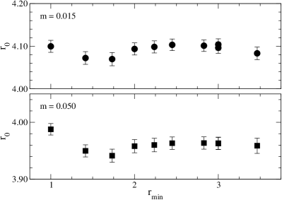
The Sommer scale is defined through the derivative of in the intermediate region of [50]
| (68) |
We fix in our simulations through the parametrization Eq. (67)
| (69) |
instead of the numerical derivative. In Fig. 22, we observe that dependence of is large and correlated to that of at . It turns out that these uncertainties partially cancel each other in the ratio Eq. (69) leading to a mild dependence of shown in Fig. 23. Therefore, as intended in Ref.[50], provides a more reliable estimate of the lattice scale than the previously-used input even through the parametrization Eq. (67) over the wide region of . Our numerical results are summarized in Table 10. We note that from three topological sectors are consistent with each other within their statistical accuracy. Its dependence is therefore ignored in the following analysis.
| fit form | ||||
|---|---|---|---|---|
| Eq. (70) | 1.60 | 0.1184(3)(17) | 0.0914(49)(57) | – |
| Eq. (70) | 0.47 | 0.1172(6)(17) | 0.145(24)(8) | -0.45(20)(2) |
| Eq. (71) | 2.00 | 8.43(2)(12) | -5.93(32)(50) | – |
| Eq. (71) | 0.46 | 8.52(4)(13) | -10.0(1.6)(0.8) | 34(13)(3) |
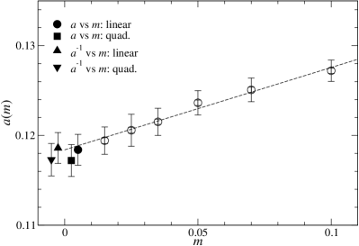
We employ an input fm to fix the scale. A quantity is then extrapolated to the chiral limit testing the following fitting functions up to quadratic order
| (70) | |||||
| (71) |
Fit parameters are summarized in Table 11. Since we have accurate data in the wide range of , the lattice spacing in the chiral limit is very stable against the choice of the fitting function as plotted in Fig. 24. We obtain
| (72) |
where the central value is from the linear form of Eq. (70) and the first error is statistical. The second error is due to the choice of the fit ranges for Eqs. (65) and (67). The third represents the uncertainty due to the choice of the chiral extrapolation form and estimated by the maximum deviation in from other three forms Eqs. (70) (quadratic) and (71).
5.1 shift
Inclusion of dynamical quarks into simulations generally makes us decrease to keep the lattice spacing fixed. The magnitude of the shift depends on the fermion formulation. A sizable negative shift, or too large bare coupling in other words, could cause problematic lattice artifacts: for instance, one may suffer from a remnant of the fundamental-adjoint phase transition [94]. In practice, some evidence of non-trivial phase structure has been found in previous unquenched simulations even at relatively fine lattice spacing fm [95, 96, 97].
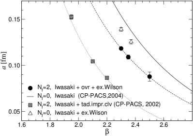
In Fig. 25, we compare the lattice spacing determined from in our and previous simulations with the Iwasaki gauge action. The shift due to the extra-Wilson fermions is not expected to be large, since effects of their high modes are cancelled in the ratio Eq. (6). This is supported by the one-loop calculation of the vacuum polarization function in Ref.[47], and Fig. 25 provides a non-perturbative confirmation.
The figure also shows that the dynamical overlap fermions lead to small shift, which is in a good accordance with an one-loop calculation in Ref.[98]. The net shift is substantially smaller than that from the tadpole-improved clover fermions. Therefore the shift is less problematic in dynamical overlap simulations even with the unphysical fermions, and this is also likely the case in three flavor QCD.
6 Locality
The locality of the overlap operator is closely related to the properties of low-lying modes of . It is proved in Ref.[100] that is exponentially local if has a positive lower bound. This does exist in our simulations by the use of the auxiliary determinant .
The central concern is therefore the size of the localization range , which should be smaller than the QCD scale . In Refs.[101, 102], it is argued that the range of is characterized by two sets of eigenmodes of : i) localized low-lying modes, whose maximum eigenvalue is denoted by in the following, and ii) extended modes with higher eigenvalues. It leads to a conjecture
| (73) |
where is the localization length of the localized modes, and represents the spectral density. The parameter is the so-called mobility edge, which separates the localized and extended modes. The prefactor of the first term follows from a steep rise in observed in Refs.[101, 102]. The extended modes govern the localization properties of through provided that and .
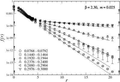
We estimate in our simulations in the following steps. First, we locate the lattice site , where the -th lowest mode has its maximum magnitude . Then a function characterizing its decay is obtained by the average
| (74) |
where represents the number of lattice points which have the same distance from . Since the spectrum of depends on the gauge configuration, we consider a range , which is divided into windows with its size of , and is averaged over the eigenmodes in each window. We calculate , where is now a window index, at and 0.050 using 10 – 40 configurations separated by 10 trajectories. Because of the small statistics, we set the bin size to 1 configuration, which possibly underestimates the statistical error quoted in this section. An example of is plotted in Fig. 26. Generally speaking, low modes decay exponentially at large and the decay rate decreases as increases.
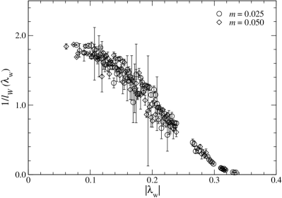
The localization length at -th window is determined by fitting at large to
| (75) |
Its dependence is plotted in Fig. 27. The mobility edge is then estimated as at which vanishes. It turns out that has small dependence but is roughly . We obtain MeV in physical units from our estimate of in Eq. (72).
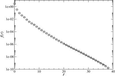
At , we also study the localization properties directly from the overlap operator multiplied to a point like quark vector
| (76) |
Here we use the taxi driver distance to avoid underestimating the localization range . We obtain
| (77) |
by an exponential fit shown in Fig. 28. Both of and therefore suggest that the overlap operator is exponentially local with a localization range smaller than in our simulations.
7 Conclusions
In this article, we simulate two-flavor QCD with dynamical overlap quarks on the reasonably large ( fm) and fine ( fm) lattice. The high statistics of 10,000 trajectories are accumulated at sea quark masses down to . The key step leading to such large-scale simulations is the suppression of the (near-)zero modes of by the auxiliary determinant. This enables us to use relatively cheap approximation of and also to avoid the substantial overhead to deal with the discontinuity of the overlap action. The use of the 5D CG algorithm, the Hasenbusch mass preconditioning and the multiple time scale MD integration also reduces the simulation cost to a large extent.
Dynamical overlap simulations are still computationally demanding compared to the domain-wall fermions [16]. The complexity of the overlap formulation however suggests that there is much room of improvement in the implementation of HMC. The low-mode preconditioning for the 5D solver is developed after this study and implemented in our latest runs [16, 15]. Further improvement in the solver algorithm, especially in the 5D solver (or alternatives) to invert , is a central concern for pushing simulations to larger volumes. The test of MD integration schemes with less discretization error and/or a further tuning of the HMC parameters and the unit trajectory length are also interesting subjects to be studied.
We are now studying various non-perturbative aspects of two-flavor QCD using the generated gauge ensembles. The chiral condensate is one of the most fundamental parameters in ChPT and has been determined in Refs.[57, 58]. Studies of the low-lying hadron spectrum [103], the kaon parameter [104] and the pion form factor [105] are in progress with paying particular attention to the consistency of their chiral behavior with ChPT. Finite size corrections based on ChPT are also important issue in these studies. Our calculation of the topological susceptibility [65] is an important step to study the nature of the QCD vacuum in fixed topological sectors. The pion mass splitting through the vector and axial-vector current correlators [106] is an example for which the exact chiral symmetry is crucial and might be difficult to study even with the domain-wall fermions. Finally, our simulations have been already extended to three-flavor QCD [16, 15] for fully realistic studies of QCD.
Acknowledgment
Numerical simulations are performed on Hitachi SR11000 and IBM System Blue Gene Solution at High Energy Accelerator Research Organization (KEK) under a support of its Large Scale Simulation Program (No. 06-13 and 07-16). We thank J. Doi, H. Samukawa and S. Shimizu of IBM Japan Tokyo Research Laboratory for assembler coding on the Blue Gene computer. This work is supported in part by the Grant-in-Aid of the Ministry of Education (No. 17340066, 17540259, 17740171, 18034011, 18340075, 18740167, 18840045, 19540286 and 19740160). The work of HF is also supported by Nishina Memorial Foundation.
References
- [1] T. Takaishi and Ph. de Forcrand, Nucl. Phys. B (Proc.Suppl.) 94, 818 (2001) [hep-lat/0011003]; Int. J. Mod. Phys. C 13, 343 (2002) [arXiv:hep-lat/0108012].
- [2] S. Aoki et al. (JLQCD collaboration), Phys. Rev. D 65, 94507 (2002) [arXiv:hep-lat/0112051].
- [3] J. C. Sexton and D. H. Weingarten, Nucl. Phys. B 380, 665 (1992).
- [4] M. Hasenbusch, Phys. Lett. B 519 (2001) 177 [arXiv:hep-lat/0107019].
- [5] M. Hasenbusch and K. Jansen, Nucl. Phys. B 659, 299 (2003) [arXiv:hep-lat/0211042].
- [6] M. Lüscher, JHEP 0305, 052 (2003) [arXiv:hep-lat/0304007].
- [7] M. Lüscher, Comput. Phys. Commun. 165, 199 (2005) [arXiv:hep-lat/0409106].
- [8] M. A. Clark and A. D. Kennedy, Phys. Rev. Lett. 98, 051601 (2007) [arXiv:hep-lat/0608015].
- [9] C. Bernard et al. (MILC collaboration), Phys. Rev. D 64, 054506 (2001) [arXiv:hep-lat/0104002]; C. Aubin et al. (MILC collaboration), ibid. D 70, 094505 (2004) [arXiv:hep-lat/0402030]; for a latest report, see C. Bernard et al. (MILC collaboration), arXiv:0710.1118 [hep-lat].
- [10] D. Kadoh et al. (PACS-CS collaboration), PoS (LATTICE 2007), 109 [arXiv:0710.3467 [hep-lat]]; N. Ukita et al. (PACS-CS collaboration), PoS (LATTICE 2007), 138 [arXiv:0710.3462 [hep-lat]]; Y. Kuramashi, PoS (LATTICE 2007), 017 [arXiv:0711.3938 [hep-lat]].
- [11] L. Del Debbio, L. Giusti, M. Lüscher, R. Petronzio and N. Tantalo, JHEP 0702, 056 (2007) [arXiv:hep-lat/0610059]; ibid. 0702, 082 (2007) [arXiv:hep-lat/0701009].
- [12] M. Göckeler et al. (QCDSF and UKQCD collaborations) PoS (LATTICE 2006), 179 [arXiv:hep-lat/0610066].
- [13] Ph. Boucaud et al. (ETM collaboration), Phys. Lett. B 650, 304 (2007) [arXiv:hep-lat/0701012]; C. Urbach, arXiv:0710.1517 [hep-lat].
- [14] C. Allton et al. (RBC and UKQCD collaborations), Phys. Rev. D 76, 014504 (2007) [arXiv:hep-lat/0701013]; P. Boyle, PoS (LATTICE 2007), 005 [arXiv:0710.5880 [hep-lat]].
- [15] S. Hashimoto et al. (JLQCD collaboration), PoS (LATTICE 2007), 101 [arXiv:0710.2730 [hep-lat]].
- [16] H. Matsufuru, PoS (LATTICE 2007) 018 [arXiv:0710.4225 [hep-lat]].
- [17] S. Dürr et al., arXiv:0710.4769 [hep-lat].
- [18] T. Ishikawa et al. (CP-PACS and JLQCD collaborations), arXiv:0704.1937 [hep-lat].
- [19] S. R. Sharpe and R. Singleton Phys. Rev. D 58, 074501 (1998) [arXiv:hep-lat/9804028].
- [20] G. Rupak and N. Shoresh, Phys. Rev. D 66, 054503 (2002) [arXiv:hep-lat/0201019].
- [21] S. Aoki, Phys. Rev. D 68, 054508 (2003) [arXiv:hep-lat/0306027].
- [22] W. Lee and S. Sharpe, Phys. Rev. D 60, 114503 (1999) [arXiv:hep-lat/9905023].
- [23] C. Bernard, Phys. Rev. D 65, 054031 (2002) [arXiv:hep-lat/0111051].
- [24] C. Aubin and C. Bernard, Phys. Rev. D 68, 034014 (2003) [arXiv:hep-lat/0304014]; ibid. D 68, 074011 (2003) [arXiv:hep-lat/0306026].
- [25] M. Della Morte, R. Hoffmann, F. Knechtli and U. Wolff (ALPHA collaboration), Comput. Phys. Commun. 165, 49 (2005) [arXiv:hep-lat/0405017].
- [26] L. Del Debbio, L. Giusti, M. Lüscher, R. Petronzio and N. Tantalo, JHEP 0602,011 (2006) [arXiv:hep-lat/0512021].
- [27] D. B. Kaplan, Phys. Lett. B 288, 342 (1992) [arXiv:hep-lat/9206013].
- [28] Y. Shamir, Nucl. Phys. B 406, 90 (1993) [arXiv:hep-lat/9303005].
- [29] V. Furman and Y. Shamir, Nucl. Phys. B 439, 54 (1995) [arXiv:hep-lat/9405004].
- [30] Y. Aoki et al. (RBC collaboration), Phys.Rev. D 72, 114505 (2005) [arXiv:hep-lat/0411006].
- [31] R. Narayanan and H. Neuberger, Nucl. Phys. B443, 305 (1995) [arXiv:hep-th/9411108].
- [32] H. Neuberger, Phys. Lett. B 417, 141 (1998) [arXiv:hep-lat/9707022]; ibid. B 427, 353 (1998) [arXiv:hep-lat/9801031].
- [33] P. H. Ginsparg and K. G. Wilson, Phys. Rev. D 25, 2649 (1982).
- [34] P. Hasenfratz, V. Laliena and F. Nidermayer, Phys. Lett. B 427, 125 (1998) [arXiv:hep-lat/9801021].
- [35] P. Hasenfratz, Nucl. Phys. B 525, 401 (1998) [arXiv:hep-lat/9802007].
- [36] M. Lüscher, Phys. Lett. B 428, 342 (1998) [arXiv:hep-lat/9802011].
- [37] P. Hasenfratz, Nucl. Phys. B (Proc.Suppl.) 63 , 53 (1998). [arXiv:hep-lat/9709110].
- [38] C. Gattringer, Phys. Rev. D 63, 114501 (2001) [arXiv:hep-lat/0003005].
- [39] W. Bietenholz and I. Hip, Nucl. Phys. B 570, 423 (2000) [arXiv:hep-lat/9902019].
- [40] A. Hasenfratz, P. Hasenfratz, D. Hierl, F. Niedermayer and A. Schäfer, PoS (LATTICE 2006), 178 [arXiv:hep-lat/0610096].
- [41] C. B. Lang, P. Majumdar and W. Ortner, Phys. Rev. D 73, 034507 (2006) [arXiv:hep-lat/0512014]; R. Frigori et al., Pos (LATTICE 2007), 114 [arXiv:0709.4582 [hep-lat]].
- [42] A. Bode, U. M. Heller, R. G. Edwards and R. Narayanan, arXiv:hep-lat/9912043.
- [43] Z. Fodor, S. D. Katz and K. K. Szabo, JHEP 0408, 003 (2004) [arXiv:hep-lat/0311010].
- [44] N. Cundy, S. Krieg, A. Frommer, Th. Lippert and K. Schilling, Nucl. Phys. B (Proc.Suppl.) 140, 841 (2005) [arXiv:hep-lat/0409029].
- [45] T. DeGrand and S. Schaefer, Phys. Rev. D 71, 034507 (2005) [arXiv:hep-lat/0412005].
- [46] N. Cundy et al., arXiv:hep-lat/0502007.
- [47] H. Fukaya et al. (JLQCD collaboration), Phys. Rev. D 74, 094505 (2006) [hep-lat/0607020].
- [48] R. Brower, S. Chandrasekharan, J. W. Negele and U.-J. Wiese, Phys. Lett. B 560, 64 (2003) [arXiv:hep-lat/0302005].
- [49] S. Aoki, H. Fukaya, S. Hashimoto and T. Onogi, Phys. Rev. D 76, 054508 (2007) [arXiv:0707.0396 [hep-lat]].
- [50] R. Sommer, Nucl. Phys. B411 (1994) 839 [arXiv:hep-lat/9310022].
- [51] H. Matsufuru et al. (JLQCD collaboration), PoS (LATTICE 2006), 031 [arXiv:hep-lat/0610026].
- [52] S. Hashimoto el al. (JLQCD collaboration), PoS (LATTICE 2006), 052 [arXiv:hep-lat/0610011].
- [53] T. Kaneko et al. (JLQCD collaboration), PoS (LATTICE 2006), 054 [arXiv:hep-lat/0610036].
- [54] N. Yamada et al. (JLQCD collaboration), PoS (LATTICE 2006), 060 [arXiv:hep-lat/0609073].
- [55] H. Fukaya et al. (JLQCD collaboration), PoS (LATTICE 2006), 050 [arXiv:hep-lat/0610024].
- [56] H. Fukaya et al. (JLQCD collaboration), PoS (LATTICE 2007), 073 [arXiv:0710.3468 [hep-lat]].
- [57] H. Fukaya et al. (JLQCD collaboration), Phys. Rev. Lett. 98, 172001 (2007) [arXiv:hep-lat/0702003].
- [58] H. Fukaya et al. (JLQCD and TWQCD collaborations), Phys. Rev. D 76, 054503 (2007). [arXiv:0705.3322 [hep-lat]]
- [59] H. Fukaya et al. (JLQCD collaboration), arXiv:0711.4965 [hep-lat].
- [60] R. Babich et al., JHEP 0601, 086 (2006) [arXiv:hep-lat/0509027].
- [61] A. Ali Khan et al. (CP-PACS collaboration), Phys. Rev. D 63, 114504 (2001) [arXiv:hep-lat/0007014].
- [62] Y. Iwasaki, preprint UTHEP-118 (1983), unpublished.
- [63] P. M. Vranas, arXiv:hep-lat/0001006; Phys. Rev. D 74, 034512 (2006) [arXiv:hep-lat/0606014].
- [64] T. Izubuchi and C. Dawson, Nucl. Phys. B (Proc.Suppl.) 106, 748 (2002).
- [65] S. Aoki et al. (JLQCD and TWQCD collaborations), arXiv:0710.1130 [hep-lat].
- [66] M. Golterman and Y. Shamir, Phys. Rev. D 76, 094512 (2007) [arXiv:0705.2928 [hep-lat]].
- [67] N. Cundy, S. Kreig, T. Lippert and A. Schäfer, arXiv:0803.0294 [hep-lat].
- [68] N. I. Akhiezer, Theory of approximation, F. Ungar, New York, 1956.
- [69] D. Ingerman, V. Druskin and L. Knizhnerman, Comm. Pure Appl. Math. 53, 1039 (2000).
- [70] A. Frommer, S. Güsken, T. Lippert, B. Nöckel and K. Schilling, Int. J. Mod. Phys. C 6, 627 (1995) [arXiv:hep-lat/9504020].
- [71] B. Jegerlehner, arXiv:hep-lat/9612014.
- [72] L. Giusti, C. Hoelbling, M. Lüscher, H. Wittig, Comput. Phys. Commun. 153, 31 (2003) [arXiv:hep-lat/0212012].
- [73] N. Cundy et al., Comput. Phys. Commun. 165 (2005) 221 [arXiv:hep-lat/0405003].
- [74] R. Narayanan and H. Neuberger, Phys. Rev. D 62, 074504 (2000) [arXiv:hep-lat/0005004].
- [75] A. Boriçi, arXiv:hep-lat/9912040; hep-lat/0402035.
- [76] R. G. Edwards, B. Joó, A. D. Kennedy, K. Orginos and U. Wenger, PoS (LAT2005) 146 [arXiv:hep-lat/0510086].
- [77] A. Ali Khan et al. (QCDSF collaboration), Phys. Lett. B 564 (2003) 235 [arXiv:hep-lat/0303026].
- [78] C. Urbach, K. Jansen, A. Shindler and U. Wenger, Comput. Phys. Commun. 174, 87 (2006) [arXiv:hep-lat/0506011].
- [79] S. Schaefer and T. DeGrand, PoS (LAT2005) 140 [arXiv:hep-lat/0508025].
- [80] G. I. Egri, Z. Fodor, S. D. Katz, K. K. Szabo, JHEP 0601, 049 (2006) [arXiv:hep-lat/0510117].
- [81] A. D. Kennedy and J. Kuti, Phys. Rev. Lett. 54, 2473 (1985).
- [82] J. Noaki et al. (JLQCD collaboration), in preparation.
- [83] H. Fukaya, S. Hashimoto, T. Hirohashi, K. Ogawa and T. Onogi, Phys. Rev. D 73, 014503 (2006) [arXiv:hep-lat/0510116].
- [84] N. Madras and A. D. Sokal, J. Stat. Phys. 50 (1988) 109.
- [85] U. Wolff, Comput. Phys. Commun. 156 (2004) 143 [arXiv:hep-lat/0306017].
- [86] U. Glässner et al. (SESAM collaboration), Nucl. Phys. B (Proc.Suppl.) 47, 386 (1996) [arXiv:hep-lat/9510001]; N. Eicker et al. (SESAM collaboratin), Phys. Lett. B 407, 290 (1997) [arXiv:hep-lat/9704019].
- [87] A. Ali Khan et al. (CP-PACS collaboration), Phys. Rev. D 65, 054505 (2002) [Erratum:ibid. D 67 059901 (2003), arXiv:hep-lat/0105015].
- [88] S. Aoki et al. (JLQCD collaboration), Phys. Rev. D 68, 054502 (2003) [arXiv:hep-lat/0212039].
- [89] Y. Namekawa et al. (CP-PACS collaboration), Phys. Rev. D 70, 074503 (2004) [arXiv:hep-lat/0404014].
- [90] B. Joó et al. (UKQCD collaboration), Phys. Rev. D 62, 114501 (2000) [arXiv:hep-lat/0005023].
- [91] A. D. Kennedy, Nucl. Phys. B (Proc.Suppl.) 140, 190 (2005) [arXiv:hep-lat/0409167].
- [92] A. Ukawa, Nucl. Phys. B (Proc.Suppl.) 106, 195 (2002).
- [93] G. S. Bali and K. Schilling, Phys. Rev. D 46, 2636 1992.
- [94] G. Bhanot, Phys. Lett. B 108, 337 (1982).
- [95] T. Blum et al., Phys. Rev. D 50, 3377 (1994) [arXiv:hep-lat/9404006].
- [96] F. Farchioni et al., Eur. Phys. J. C 39, 421 (2005) [arXiv:hep-lat/0406039].
- [97] S. Aoki et al. (JLQCD collaboration), Phys. Rev. D 72, 054510 (2005) [arXiv:hep-lat/0409016].
- [98] C. Alexandrou, H. Panagopoulos and E. Vicari, Nucl. Phys. B 571, 257 (2000) [arXiv:hep-lat/9909158].
- [99] S. Takeda et al. (CP-PACS collaboration), Phys. Rev. D 70, 074510 (2004) [arXiv:hep-lat/0408010].
- [100] P. Hernández, K. Jansen and M. Lüscher, Nucl. Phys. B 552, 363 (1999) [arXiv:hep-lat/9808010].
- [101] M. Golterman and Y. Shamir, Phys. Rev. D 68, 074501 (2003) [arXiv:hep-lat/0306002].
- [102] M. Golterman, Y. Shamir and B. Svetitsky, Phys. Rev. D 72, 034501 (2005) [arXiv:hep-lat/0503037].
- [103] J. Noaki et al. (JLQCD collaboration), PoS (LATTICE 2007) 126 [arXiv:0710.0929 [hep-lat]].
- [104] N. Yamada et al. (JLQCD collaboration), arXiv:0710.0462 [hep-lat].
- [105] T. Kaneko et al. (JLQCD collaboration), PoS (LATTICE 2007) 148 [arXiv:0710.2390 [hep-lat]].
- [106] E. Shintani et al. (JLQCD collaboration), PoS (LATTICE 2007) 134 [arXiv:0710.0691 [hep-lat]].