Theory of Excitonic States in Medium-Sized Quantum Dots

Abstract

In a quantum dot with dozens of electrons, an approximation beyond Tamm-Dankoff is used to construct the quantum states with an additional electron-hole pair, i.e. the “excitonic” states. The lowest states mimic the non-interacting spectrum, but with excitation gaps renormalized by Coulomb interactions. At higher excitation energies, the computed density of energy levels shows an exponential increase with energy. In the interband absorption, we found a background level in the quasicontinuum of states rising linearly with the excitation energy. Above this background, there are distinct peaks related to single resonances or to groups of many states with small interband dipole moments.

I Introduction

Semiconductor quantum dots are like anisotropic Thomson atoms. Most of their electronic and optical properties are, by now, well studied QDots_Review . The typical energy scales determining these properties are the following: the in-plane confinement strength, $\hbar\omega$, which also defines the unit of length, the characteristic Coulomb energy, $\beta$, and the characteristic energy along the symmetry axis, $E_{z}$. The ratio $\beta/\hbar\omega$ is an indicator of the role played by Coulomb interactions in the dot. In the strong confinement regime, $\beta/\hbar\omega\ll 1$, which we encounter in self-assembled structures, quantum dots are like real atoms, with correlation energies reaching only a few percents of the total energy. On the other hand, for $\beta/\hbar\omega\gg 1$, correlations are strong, and there could be even premonitions of Wigner crystalization for large enough dots.

The excited states of a quantum dot, as in most quantum systems, subscribe to a general picture of a few low-lying “oscillator” states followed by a quasi-continuum of excitations. Typically, the low lying states determine most of the optical properties. But there are situations in which higher excitations play a key role. Raman scattering or PLE experiments with excitation energies $40-60$ meV above band gap, for instance, sense high interband excitations. On the other hand, the density of energy levels in the quasi-continuum obeys a simple exponential rule with excitation energy, known in Nuclear Physics as the Constant Temperature Approximation (CTA) CTA_in_Nucl_Phys . In paper [PRB_con_Capote, ], we corroborated this picture for the intraband excitations of few-electron quantum dots in a magnetic field.

In the present paper, we focus on the interband excitations. A medium-size dot, charged with $42$ electrons, under intermediate confinement regime ($\beta/\hbar\omega\approx 0.6$) is studied, a situation typical of etched dots. As it will be shown below, the obtained low-lying spectrum is similar to the spectrum of the non-interacting model, but with values renormalized by Coulomb interactions. The quasi-continuum of states follows the CTA, as expected.

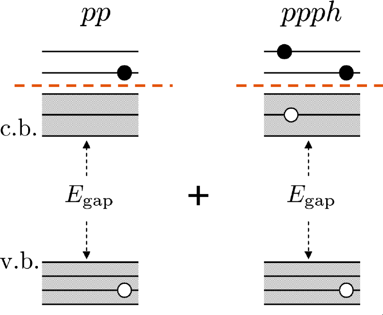
Figure 1: (Color online) The pp-TDA and ppph contributions to the wave function of the excitonic states.

For a dot with $42$ electrons, no exact diagonalization calculations are possible and we should resort to approximations. We will use a kind of Quantum Chemistry Configuration Interaction Method (CI) C_I in which the starting point is the Hartree-Fock (HF) solution for the $42$-electron problem. Excitations over the HF solution conform the basis functions in which our Hamiltonian is to be diagonalized. The simplest set of excitations, one additional electron in the conduction band (CB) and one hole in the valence band (VB), is usually called pp-Tamm-Dankoff approximation (pp-TDA) in Nuclear Physics Ring . The valence-band hole is treated as a quasiparticle with its own dispersion relation. Excitonic states are, thus, states with two additional “particles” above the HF solution. The next set in increasing complexity includes excitations with an additional electron above the Fermi level and a hole below the Fermi level in the CB. We will call it the ppph contribution. A schematic representation of the pp-TDA and ppph contributions to the wave function of the excitonic states is given in Fig. 1. We will truncate the basis of functions at this stage.

The reason for including next-to-leading order excitations in the basis functions, i.e. going beyond pp-TDA, is the following. It is well known that the pp-TDA underestimates the density of energy levels already for relatively low excitation energies. A correct level density could be crucial in the description of Raman scattering events with laser excitation energy well above band gap, which is our next goal. A particularly interesting question is why the so called outgoing resonances, presumably a result of higher order Raman processes Danan_&_Pinczuk , give stronger contribution to the Raman spectrum than the usual second-order Raman amplitude.

II Formalism

As mentioned above, the starting point in our formalism is the HF solution for the $42$-electron problem. The HF equations and the way we solve them are described elsewhere Alain_PRB ; Alain_thesis . We use the following set of parameters: $m_{e}=0.067~{}m_{0}$, (a GaAs quantum dot), $\hbar\omega_{e}=12$ meV (the confinement energy for electrons), and $\beta=7.07$ meV. The latter value comes from the expression: $\beta=0.6~{}e^{2}/(4\pi\epsilon_{0}\kappa l)$, where the relative dielectric constant is $\kappa=12.8$, $l$ is the oscillator length, and the factor 0.6 takes account of the quasibidimensionality of the structure. Only one electron sub-band in the z-direction is considered, and the value of $E_{z}^{(e)}$ is used to control the effective band gap of the nanostructure.

The HF states for the hole in the VB are found from the Kohn-Luttinger Hamiltonian, in which a term accounting for the background potential created by the $42$ electrons is included Alain_PRB ; Alain_thesis .

For the interband excitations of the dot, i.e. many-particle wave functions with $43$ electrons and one hole, we write the ansatz,

$$|int\rangle = \left(\sum_{\sigma,\tau}V_{\sigma\tau}e^{\dagger}_{\sigma}h^{\dagger}_{\tau}+\sum_{\sigma,\rho,\lambda,\tau}Z_{\sigma\rho\lambda\tau}e^{\dagger}_{\sigma}e^{\dagger}_{\rho}e_{\lambda}h^{\dagger}_{\tau}\right)|HF\rangle$$ (1)

$$= Q^{\dagger}|HF\rangle.$$

$\sigma$ and $\rho$ are electronic states above the Fermi level, and $\lambda$ is a state below the Fermi level of electrons. We restrict the second sum in Eq. (1) to $\sigma>\rho$ in order to avoid overcounting. This second sum is the term beyond pp-TDA, not included in previous computations of interband excitations Alain_PRB ; Alain_thesis .

Due to the peculiarities of Coulomb interactions, the Kohn-Luttinger Hamiltonian, and the central confinement potential, the interband excitations are characterized by two quantum numbers, $F$ and $S_{z}$. It means that the single-particle states entering the first and second sums of Eq. (1) should satisfy, respectively, the first and second rows of the following equalities:

$$F = l_{\sigma}+l_{\tau}-m_{j}$$ (2)

$$= l_{\sigma}+l_{\rho}-l_{\lambda}+l_{\tau}-m_{j},$$

$$S_{z} = S_{\sigma}$$ (3)

$$= S_{\sigma}+S_{\rho}-S_{\lambda}.$$

Here $l$ are (orbital) angular momentum, $m_{j}$ - (band) hole angular momentum, and $S$ - (electron) spin quantum numbers. Of course, these magnitudes correspond to projections along the $z$-axis.

The coefficients $V$ and $Z$ (the wave functions) and the excitation energies with respect to the HF state are computed from the following eigenvalue problem, in close analogy with the TDA Ring

$$[H,Q^{\dagger}]|HF\rangle=\Delta E_{int}~{}Q^{\dagger}|HF\rangle,$$ (4)

where $H$ is the many-particle electron-hole Hamiltonian

$$H=T_{e}+T_{h}+V_{ee}+V_{eh}.$$ (5)

The $T$ are one-body operators, and $V$ refer to Coulomb interactions. Let us stress that electron-hole exchange, usually of the order of $\mu$eV in these structures, is neglected. The explicit matrix form of Eq. (4) is presented in Appendix A for completeness. We use energy cutoffs of 90 meV to reduce the dimensions of the resulting matrices to around 12000. Eigenvalues and eigenvectors (the wave functions) are obtained by numerical diagonalization.

III The lowest excitonic states

The solution of Eq. (4) provides us the wave functions and energies of the interband excitations of the dot (the excitonic states). In this section we focus on the lowest states.

A sample of results is shown in Fig. 2(a). Energies are measured with respect to $E_{HF}+E_{z}^{(e)}$. States with quantum numbers $F=-3/2$, $S_{z}=1/2$ are represented in the figure. With increasing energy we observe first a pair of states followed by a group of four states, and then a quasi-continuum of excitations. This sequence can be understood in terms of the non-interacting picture of electrons and holes.

Figure 2: (a) The low-lying interband excitations in the model quantum dot. States with $F=-3/2$, $S_{z}=1/2$ are drawn. Results from the non-interacting picture are also shown for comparison. (b) Increase in the density of energy levels due to the ppph component.

Our model dot with $42$ electrons has $6$ filled $2D$ oscillator shells. We should add an electron-hole pair to construct an interband excitation. The electron should then be added to the 7th shell. The possible angular momentum values are $l_{e}=-6,-4,\dots,6$. The hole orbital state, on his hand, can be the first oscillator state with $l_{h}=0$. As we are talking about $F=-3/2$ states, only two combinations remain: $l_{e}=0$, $mj=3/2$ and $l_{e}=-2$, $mj=-1/2$. That is, one heavy and one ligth hole exciton that, because of the assumed $25$ nm width of the dot in the $z$-direction, are very close in energy (1.5 meV). The next set of 4 states are related to hole excitations, i.e. the hole occupies one oscillator state of the 2nd shell. We choose the confinement frequency for holes in such a way that the oscillator length is unique, meaning that electrons and holes are confined in the same spatial region. For heavy holes, for example, it means that $\omega_{hh}=m_{e}\omega_{e}/m_{hh}$. As a result, excitations energies for holes are smaller, of around 5 meV. Next, we reach a group, more numerous, of states built up from one-$\hbar\omega$ electron excitations (12 meV) or two-$\hbar\omega$ hole excitations.

Following this non-interacting picture, we can assign the first two levels to heavy-hole and ligth-hole excitons, the next four to hole excitations to the 2nd oscillator shell, and we can relate the quasi-continuum of states to electron excitations to the 8th shell and hole excitations to the third shell. The effects of Coulomb interactions are apparent in Fig. 2(a): energy values are pushed down, energy gaps are reduced and a quasi-continuum of levels appear at excitation energies even below $\hbar\omega_{e}=12$ meV.

In Fig. 2(b) we illustrate the main effects of the ppph component on the energy levels. As compared with the pp-TDA, we get small variations of the ground state energy (of around 3 meV) and the gap to the first quartet of states. But, for excitation energies above 10 meV a significant increase in the level density is observed. In the next section a more detailed study of the density of energy levels is carried on.

IV The Constant Temperature Approximation (CTA)

It can be verified that the CTA is a good approximation for the density of energy levels at relatively small excitation energies, starting from the quasi-continuum of states.

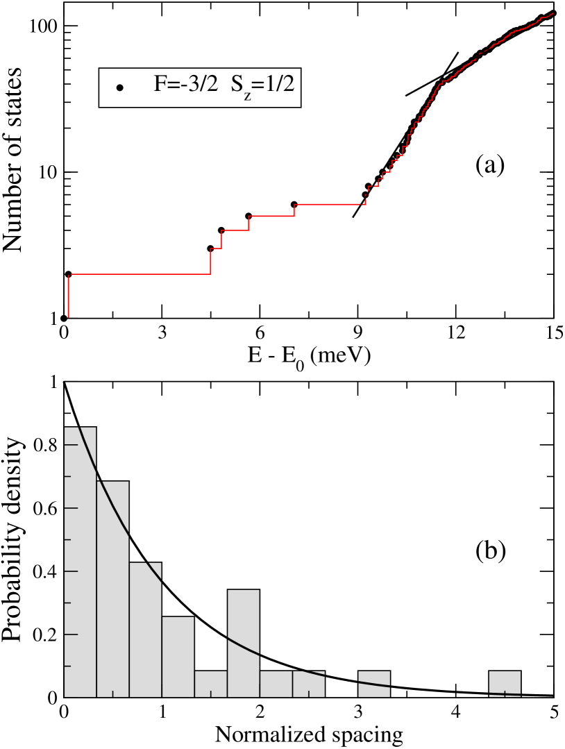
Figure 3: (Color online) (a) Increase in the number of levels as predicted by the CTA for states with 9 meV $<\Delta E<$ 15 meV. (b) Probability distribution of level spacing for excitonic states in the interval 9 meV $<\Delta E<$ 12 meV.

We show in Fig. 3(a) the excitonic sector with quantum numbers $F=-3/2$, $S_{z}=1/2$. Excitation energies, measured with respect to the lowest state in this sector, run in the interval 0 - 15 meV. A perfect exponential behaviour is apparent in the regions 9 meV $<\Delta E<$ 12 meV and 12 meV $<\Delta E<$ 15 meV. In these intervals, the number of states can be fitted to:

$$N=N_{0}\exp\left(\frac{\Delta E}{\Theta}\right),$$ (6)

where: $N_{0}=4.472\times 10^{-3}$, $\Theta=1.268$ meV for 9 meV $<\Delta E<$ 12 meV, and $N_{0}=1.145$, $\Theta=3.183$ meV for 12 meV $<\Delta E<$ 15 meV.

We guess that a simple qualitative relation should exist between the temperature parameter, $\Theta$ (the slope), and the system parameters. Indeed, in a scaled formulation GPP $\Theta$ should be proportional to $\hbar\omega_{e}$, simply because of dimensional arguments. The number of electrons, $N_{e}$, and the scaled Coulomb strength, $\hat{\beta}=\beta/(\hbar\omega_{e})$ should appear in the combination $N_{e}^{1/4}\hat{\beta}$.GPP We expect the following dependence: $\Theta\sim\hbar\omega_{e}/(N_{e}^{1/4}\hat{\beta})^{2/3}$. A verification of the above dependence requires extensive calculations and is delayed for a future work.

The slope discontinuity at $\Delta E\approx 12$ meV is a reminiscence of shell structure. Indeed, if there were a gap between perfect shells, then the curve would be flat immediatly after $\Delta E\approx 12$ meV. Coulomb interaction is responsible for filling the “gap” region, 12 meV $<\Delta E<$ 15 meV, with levels.

The interpretation of levels in the interval 9 meV $<\Delta E<$ 12 meV as a “distorted shell” is also reinforced by the distribution of spacing between neighbourgh levels, as shown in Fig. 3(b). The probability density vs spacing, normalized to the mean level spacing, which in the present situation is 0.067 meV, is shown to follow a Poissonian dependence, indicating a regular region of phase space Level_spacing_in_Q_Systems . This statement proves that the CTA is not necessarily related to chaos in the excitation spectrum.

In conclusion, the quasi-continuum of excitonic states for 9 meV $<\Delta E<$ 12 meV $\approx\hbar\omega_{e}$ exhibits regular or quasi-integrable behaviour and is well described by the CTA. Above this interval, an abrupt change in the temperature parameter is reminiscent of shell strucure in the model.

V Interband Absorption

Interband absorption at normal incidence is characterized by the creation of electron-hole pairs mainly in monopole states, $l_{e}+l_{h}=0$. This means low values of $|F|$.

The transition matrix element for absorption is given by

$$\langle int|H^{(-)}|i\rangle=\sum_{\sigma,\tau}V_{\sigma\tau}^{*}b_{\sigma\tau},$$ (7)

where the initial state is the HF state for the $42$-electron system, and $H^{(-)}$ is the light-matter coupling Hamiltonian corresponding to the absorption of a photon and creation of a pair. An explicit expresion for $H^{(-)}$ is given in Refs. [ORA, ; Alain_thesis, ]. The matrix elements $b_{\sigma\tau}$ are explicitly given in Ref. [Alain_PRB, ], where they are termed band-orbital factors (see Eq. (30) of that paper). Notice that only the first part of the wave function (1) enters the matrix element (7). This is the result of treating the ground state in the Hartree-Fock approximation. 1p1h corrections would not modify Eq. (7) because the Hartree-Fock state is orthogonal to 1p1h corrections Ring .

We show in Fig. 4(a) the computed zero-temperature interband absorption in our model quantum dot. We consider normal incidence and linear polarization. The absorption intensity has contributions from four sets of states, that is $(F,S_{z})$=(-3/2,1/2), (3/2,-1/2), (-1/2,-1/2) and (1/2,1/2). A Lorentzian broadening of the spectral lines is assumed. The energy widths, $\Gamma_{int}$, are choosen in the following way: $\Gamma_{int}=0.5$ meV for $\Delta E<35$ meV, and $\Gamma_{int}=2.0$ for $\Delta E>35$ meV, where $\Delta E$ is the energy difference with respect to the first excitonic state, and the value 35 meV is the LO phonon energy in GaAs. Our ansatz for $\Gamma_{int}$ expresses the fact that the opening of the channel for the emission of a LO phonon broadens the excitonic levels.

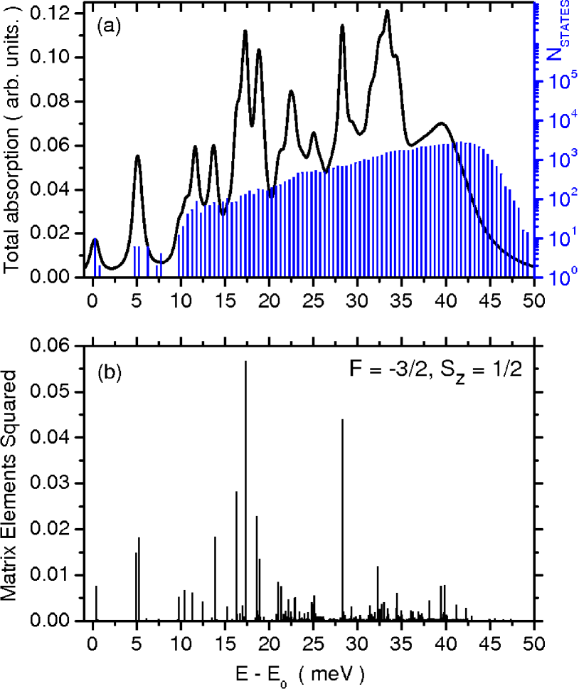
Figure 4: (Color online) (a) Interband absorption in our model dot and the density of energy levels. (b) Contribution to the absorption by the set of states with quantum numbers $F=-3/2$, $S_{z}=1/2$.

The absorption spectrum has the usual form. First, a few isolated peaks, and then a quasicontinuum. We have superimposed in Fig. 4(a) a histogram with the density of energy levels, in logarithmic scale. To construct the histogram, we used an energy width equal to $\Gamma_{int}$, that is 0.5 meV. The decrease of the density of states for $\Delta E\geq 45$ meV is an artifact related to the truncation of Hilbert space. It becomes evident that in the quasicontinuum there is a background absorption intensity roughly proportional to the logarithm of the level density, i.e. to the excitation energy $\Delta E$ (because of the CTA). We notice that this is the dependence that follows for absorption in the independent-particle picture for electrons in a harmonic potential. Above this background level, we observe distinct peaks.

The contribution to the interband absorption by the set of states with quantum numbers $F=-3/2$, $S_{z}=1/2$ is sketched in Fig. 4(b). The comparison with Fig.4(a) reveals that there are peaks associated to one (or a few) excitonic states with strong interband dipole moments, but there are also peaks due to the contribution of many states with relatively small dipole moments. The latter are better understood as broad resonances, but they should be distinguished from the background intensity created by the “single-pair” excitations.

VI Concluding remarks

In the present paper, we have computed the excitonic states in a relatively large quantum dot by using a Configuration Interation scheme. This is an ab-initio procedure, fully variational. The only approximations in it are the effective mass description of electrons, the Kohn-Luttinger description of holes in the valence band and the harmonic model for the dot. To the best of our knowledge, this is the first calculation of such kind in the literature.

For the sake of simplicity in the presentation, we used a closed-shell situation, 42 electrons, in which the ground state is characterized by quantum numbers $L_{total}=0$, and $S=0$. However, our scheme works properly also for open-shell dots and, with appropiate 2p2h corrections, provides quantum numbers for the ground state in accordance with Hund’s rules2p2h . Comparison with exact calculations for few-electron dots shows excelent agreement 2p2h .

The main results of the paper are the following: (a) A picture for the low-lying states in which the role of Coulomb interactions is made evident, (b) A universal parametrization of the density of energy levels for excitation energies greater than 1 $\hbar\omega$, and (c) A picture for the interband absorption made up from peaks of different nature and a background level in the quasicontinuum rising linearly with energy.

The work may be continued along different lines. A natural extension is the description of biexcitonic states. The verification of universality of the CTA in the level density of quantum systems is also worth trying. Finally, the obtained excitonic states can be used in the computation of Raman cross sections for laser excitation energies well above band gap. Reasearch along these directions is currently in progress.

Appendix A Eq. (4) in matrix form

Eq. (1) for the $Q^{\dagger}$ operator makes evident the basis functions used in the construction of the excitonic states. They are of two kinds:

$$e^{\dagger}_{\sigma}h^{\dagger}_{\tau}|HF\rangle,$$ (8)

and

$$e^{\dagger}_{\sigma}e^{\dagger}_{\rho}e_{\lambda}h^{\dagger}_{\tau}|HF\rangle.$$ (9)

If Eq. (4) is projected onto these basis functions, we get the following system of equations:

$$\sum_{\sigma\tau}\langle HF|[h_{\tau^{\prime}}e_{\sigma^{\prime}},[H,e^{\dagger}_{\sigma}h^{\dagger}_{\tau}]]|HF\rangle V_{\sigma\tau} + \sum_{\sigma\rho\lambda\tau}\langle HF|[h_{\tau^{\prime}}e_{\sigma^{\prime}},[H,e^{\dagger}_{\sigma}e^{\dagger}_{\rho}e_{\lambda}h^{\dagger}_{\tau}]]|HF\rangle Z_{\sigma\rho\lambda\tau}$$ (10)

$$= \Delta E_{int}\sum_{\sigma\tau}\langle HF|[h_{\tau^{\prime}}e_{\sigma^{\prime}},e^{\dagger}_{\sigma}h^{\dagger}_{\tau}]|HF\rangle V_{\sigma\tau},$$

$$\sum_{\sigma\tau}\langle HF|[h_{\tau^{\prime}}e^{\dagger}_{\lambda^{\prime}}e_{\rho^{\prime}}e_{\sigma^{\prime}},[H,e^{\dagger}_{\sigma}h^{\dagger}_{\tau}]]|HF\rangle V_{\sigma\tau}\ + \sum_{\sigma\rho\lambda\tau}\langle HF|[h_{\tau^{\prime}}e^{\dagger}_{\lambda^{\prime}}e_{\rho^{\prime}}e_{\sigma^{\prime}},[H,e^{\dagger}_{\sigma}e^{\dagger}_{\rho}e_{\lambda}h^{\dagger}_{\tau}]]|HF\rangle Z_{\sigma\rho\lambda\tau}$$ (11)

$$= \Delta E_{int}\sum_{\sigma\rho\lambda\tau}\langle HF|[h_{\tau^{\prime}}e^{\dagger}_{\lambda^{\prime}}e_{\rho^{\prime}}e_{\sigma^{\prime}},e^{\dagger}_{\sigma}e^{\dagger}_{\rho}e_{\lambda}h^{\dagger}_{\tau}]|HF\rangle Z_{\sigma\rho\lambda\tau},$$

where $\Delta E_{int}$ is the excitation energy, measured with respect to the ground state of the $N_{e}$-electron system, and $H$ is the quantum dot Hamiltonian. These equations can be rewritten in a more compact form:

$$\left(\matrix{A&C\cr C^{t}&B}\right)\left(\matrix{V\cr Z}\right)=\Delta E_{int}\left(\matrix{V\cr Z}\right).$$ (12)

The matrix elements entering Eq. (12) are computed by means of the following expressions:

$$\langle\sigma\tau|A|\sigma^{\prime}\tau^{\prime}\rangle\ =\ (\epsilon_{\sigma}+\epsilon_{\tau})\delta_{\sigma\sigma^{\prime}}\delta_{\tau\tau^{\prime}}-\beta\langle\sigma^{\prime}\tau^{\prime}|\frac{1}{r_{eh}}|\sigma\tau\rangle,$$ (13)

$$\langle\sigma\rho\lambda\tau|B|\sigma^{\prime}\rho^{\prime}\lambda^{\prime}\tau^{\prime}\rangle\ = \ (\epsilon_{\sigma}+\epsilon_{\rho}+\epsilon_{\tau}-\epsilon_{\lambda})\delta_{\sigma\sigma^{\prime}}\delta_{\rho\rho^{\prime}}\delta_{\tau\tau^{\prime}}\delta_{\lambda\lambda^{\prime}}$$ (14)

$$- \ \beta\left(\langle\rho^{\prime}\sigma^{\prime}|\frac{1}{r_{e}}|\overline{\rho\sigma}\rangle\delta_{\tau\tau^{\prime}}\delta_{\lambda\lambda^{\prime}}+\langle\lambda\rho^{\prime}|\frac{1}{r_{e}}|\overline{\rho\lambda^{\prime}}\rangle\delta_{\tau\tau^{\prime}}\delta_{\sigma\sigma^{\prime}}+\langle\lambda\sigma^{\prime}|\frac{1}{r_{e}}|\overline{\sigma\lambda^{\prime}}\rangle\delta_{\tau\tau^{\prime}}\delta_{\rho\rho^{\prime}}\right.$$

$$+ \left.\langle\lambda\rho^{\prime}|\frac{1}{r_{e}}|\overline{\lambda^{\prime}\sigma}\rangle\delta_{\tau\tau^{\prime}}\delta_{\rho\sigma^{\prime}}+\langle\lambda\sigma^{\prime}|\frac{1}{r_{e}}|\overline{\lambda^{\prime}\rho}\rangle\delta_{\tau\tau^{\prime}}\delta_{\sigma\rho^{\prime}}\right)\ -\ \beta\left(\langle\sigma^{\prime}\tau^{\prime}|\frac{1}{r_{eh}}|\sigma\tau\rangle\delta_{\rho\rho^{\prime}}\delta_{\lambda\lambda^{\prime}}\right.$$

$$- \left.\langle\rho^{\prime}\tau^{\prime}|\frac{1}{r_{eh}}|\sigma\tau\rangle\delta_{\rho\sigma^{\prime}}\delta_{\lambda\lambda^{\prime}}-\langle\lambda\tau^{\prime}|\frac{1}{r_{eh}}|\lambda^{\prime}\tau\rangle\delta_{\rho\rho^{\prime}}\delta_{\sigma\sigma^{\prime}}-\langle\sigma^{\prime}\tau^{\prime}|\frac{1}{r_{eh}}|\rho\tau\rangle\delta_{\sigma\rho^{\prime}}\delta_{\lambda\lambda^{\prime}}\right.$$

$$+ \left.\langle\rho^{\prime}\tau^{\prime}|\frac{1}{r_{eh}}|\rho\tau\rangle\delta_{\sigma\sigma^{\prime}}\delta_{\lambda\lambda^{\prime}}\right),$$

$$\langle\sigma\rho\lambda\tau|C|\sigma^{\prime}\tau^{\prime}\rangle\ =\ \beta\left(\langle\sigma^{\prime}\lambda|\frac{1}{r_{e}}|\overline{\rho\sigma}\rangle\delta_{\tau\tau^{\prime}}-\langle\lambda\tau^{\prime}|\frac{1}{r_{eh}}|\sigma\tau\rangle\delta_{\rho\sigma^{\prime}}+\langle\lambda\tau^{\prime}|\frac{1}{r_{eh}}|\rho\tau\rangle\delta_{\sigma\sigma^{\prime}}\right),$$ (15)

$$\langle\sigma\tau|C^{t}|\sigma^{\prime}\rho^{\prime}\lambda^{\prime}\tau^{\prime}\rangle\ =\ \beta\left(\langle\rho^{\prime}\sigma^{\prime}|\frac{1}{r_{e}}|\overline{\sigma\lambda^{\prime}}\rangle\delta_{\tau\tau^{\prime}}-\langle\sigma^{\prime}\tau^{\prime}|\frac{1}{r_{eh}}|\lambda^{\prime}\tau\rangle\delta_{\sigma\rho^{\prime}}+\langle\rho^{\prime}\tau^{\prime}|\frac{1}{r_{eh}}|\lambda^{\prime}\tau\rangle\delta_{\sigma\sigma^{\prime}}\right),$$ (16)

where we used the notation $\langle ij||\overline{kl}\rangle=\langle ij||kl\rangle-\langle ij||lk\rangle$ for the Coulomb matrix elements, $\epsilon_{i}$ denotes the energy of the Hartree-Fock state $i$, and $\beta$ is the Coulomb interaction strength.

References

- (1) Y. Masumoto and T. Takagahara (eds.), Semiconductor Quantum Dots (Springer, Berlin, 2002).
- (2) T. Ericson, Adv. Phys. 9, 425 (1960); A. Gilbert, A.G.W. Cameron, Can. J. Phys. 43, 1446 (1965).
- (3) A. Gonzalez and R. Capote, Phys. Rev. B 66, 113311 (2002).
- (4) C.J. Cramer, Essentials of Computational Chemistry: Theories and Models (John Wiley & Sons, Chichester, 2006).
- (5) P. Ring and P. Schuck, The Nuclear Many-Body Problem (Springer-Verlag, New-York, 1980).
- (6) G. Danan, A. Pinczuk, J.P. Valladares, et al, Phys. Rev. B 39, 5512 (1989).
- (7) A. Delgado, A. Gonzalez, and D.J. Lockwood, Phys. Rev. B 69, 155314 (2004).
- (8) A. Delgado, Inelastic Light Scattering by Electronic Excitations in Artificial Atoms (Ph. D. Thesis, Havana, Dec. 2006).
- (9) A. Gonzalez, B. Partoens and F.M. Peeters, Phys. Rev. B 56, 15740 (1997).
- (10) A. Gonzalez and A. Delgado, Physica E 27, 5 (2005).
- (11) O. Bohigas, M.J. Giannoni, and C. Schmit, Phys. Rev. Lett. 52, 1 (1984); F. Haake, Quantum Signatures of Chaos (Springer, Berlin, 1991).
- (12) A. Delgado, A. Odriazola, and A. Gonzalez, to be submitted.