Full optimization of Jastrow-Slater wave functions with application to the first-row atoms and homonuclear diatomic molecules

Abstract

We pursue the development and application of the recently-introduced linear optimization method for determining the optimal linear and nonlinear parameters of Jastrow-Slater wave functions in a variational Monte Carlo framework. In this approach, the optimal parameters are found iteratively by diagonalizing the Hamiltonian matrix in the space spanned by the wave function and its first-order derivatives, making use of a strong zero-variance principle. We extend the method to optimize the exponents of the basis functions, simultaneously with all the other parameters, namely the Jastrow, configuration state function and orbital parameters. We show that the linear optimization method can be thought of as a so-called augmented Hessian approach, which helps explain the robustness of the method and permits us to extend it to minimize a linear combination of the energy and the energy variance. We apply the linear optimization method to obtain the complete ground-state potential energy curve of the C₂ molecule up to the dissociation limit, and discuss size consistency and broken spin-symmetry issues in quantum Monte Carlo calculations. We perform calculations of the first-row atoms and homonuclear diatomic molecules with fully optimized Jastrow-Slater wave functions, and we demonstrate that molecular well depths can be obtained with near chemical accuracy quite systematically at the diffusion Monte Carlo level for these systems.

I Introduction

Quantum Monte Carlo (QMC) methods (see e.g. Refs. Hammond et al., 1994; Nightingale and Umrigar, 1999; Foulkes et al., 2001) constitute an alternative to standard quantum chemistry approaches for accurate calculations of the electronic structure of atoms, molecules and solids. The two most commonly used variants, variational Monte Carlo (VMC) and diffusion Monte Carlo (DMC), use a flexible trial wave function, generally consisting for atoms and molecules of a Jastrow factor multiplied by a short expansion in configuration state functions (CSFs), each consisting of a linear combination of Slater determinants of orbitals expanded in a localized one-particle basis. To fully benefit from the considerable flexibility in the form of the wave function, it is crucial to be able to efficiently optimize all the parameters in these wave functions.

In recent years, a lot of effort has been devoted to developing efficient methods for optimizing a large number of parameters in QMC wave functions. One the most effective approaches is the linear optimization method of Refs. Toulouse and Umrigar, 2007 and Umrigar et al., 2007. This is an extension of the zero-variance generalized eigenvalue equation approach of Nightingale and Melik-Alaverdian Nightingale and Melik-Alaverdian (2001) to arbitrary nonlinear parameters, and it permits a very efficient and robust energy minimization in a VMC framework. This method was applied successfully to the simultaneous optimization of Jastrow, CSF and orbital parameters of Jastrow-Slater wave functions for some all-electron atoms and molecules in Refs. Toulouse and Umrigar, 2007 and Toulouse et al., 2007, and for the C₂ and Si₂ molecules with pseudopotentials in Ref. Umrigar et al., 2007. It has also been applied in Ref. Brown et al., 2007 for optimizing Jastrow, CSF and backflow parameters to obtain very accurate wave functions for the first-row atoms.

In this paper, we pursue the development and application of the linear optimization method. We extend the method to optimize the exponents of the basis functions, simultaneously with all the other parameters, a capacity rarely available in standard quantum chemistry methods (see, however, Refs. Tachikawa et al., 1998, 1999; Tachikawa and Osamura, 2000). This uses a slight generalization of the parametrization employed for Jastrow-Slater wave functions to allow nonorthogonal orbitals. Also, we show that the linear optimization method can be thought of as a so-called augmented Hessian approach. This allows us to clearly establish the connection between the linear optimization method and a stabilized Newton optimization method, helping to explain the robustness of the approach. Moreover, this formulation permits us to extend the method to minimize a linear combination of the energy and the energy variance, as done in Ref. Umrigar and Filippi, 2005 with the Newton method. We then apply the linear optimization method to obtain the complete ground-state potential energy curve of the C₂ molecule up to the dissociation limit, and discuss size consistency and broken spin-symmetry issues in QMC calculations. Finally, we perform calculations of the first-row atoms and homonuclear diatomic molecules with fully optimized Jastrow-Slater wave functions, and we demonstrate that molecular well depths can be obtained with near chemical accuracy quite systematically at the DMC level for these systems.

When not explicitly indicated, Hartree atomic units are assumed throughout this work.

II Wave function optimization

II.1 Wave function parametrization

To optimize a large number of parameters of a wave function, it is important to use a convenient and efficient parametrization that eliminates redundancies. We use an $N$-electron Jastrow-Slater wave function parametrized as (see Ref. Toulouse and Umrigar, 2007)

$$|\Psi(\mathbf{p})\rangle=\hat{J}(\bm{\alpha})e^{\hat{\kappa}(\bm{\kappa},\,\bm{\zeta})}\sum_{I=1}^{N_{\text{CSF}}}c_{I}|C_{I}(\bm{\zeta})\rangle,$$ (1)

where $\hat{J}(\bm{\alpha})$ is a Jastrow operator, $e^{\hat{\kappa}(\bm{\kappa},\,\bm{\zeta})}$ is an orbital transformation operator, and $|C_{I}(\bm{\zeta})\rangle$ are configuration state functions (CSFs). The parameters to be optimized, collectively designated by $\mathbf{p}=(\bm{\alpha},\mathbf{c},\bm{\kappa},\bm{\zeta})$, are the Jastrow parameters $\bm{\alpha}$, the CSF parameters $\mathbf{c}$, the orbital rotation parameters $\bm{\kappa}$ and the basis exponent parameters $\bm{\zeta}$.

We use a flexible Jastrow factor consisting of the exponential of the sum of electron-nucleus, electron-electron and electron-electron-nucleus terms, written as systematic polynomial and Padé expansions Umrigar (see also Refs. Filippi and Umrigar, 1996; Güçlü et al., 2005). Each CSF is a short linear combination of products of spin-up and spin-down Slater determinants $|D_{\mathbf{k}}^{\uparrow}(\bm{\zeta})\rangle$ and $|D_{\mathbf{k}}^{\downarrow}(\bm{\zeta})\rangle$

$$|C_{I}(\bm{\zeta})\rangle=\sum_{\mathbf{k}}d_{I,\mathbf{k}}|D_{\mathbf{k}}^{\uparrow}(\bm{\zeta})\rangle|D_{\mathbf{k}}^{\downarrow}(\bm{\zeta})\rangle,$$ (2)

where the coefficients $d_{I,\mathbf{k}}$ are fully determined by the spatial and spin symmetries of the state considered. The $N_{\uparrow}$-electron and $N_{\downarrow}$-electron Slater determinants are generated from the set of non-necessarily orthonormal orbitals at the current optimization step, $|D_{\mathbf{k}}^{\uparrow}(\bm{\zeta})\rangle=\hat{a}^{0{\dagger}}_{k_{1}\uparrow}(\bm{\zeta})\hat{a}^{0{\dagger}}_{k_{2}\uparrow}(\bm{\zeta})\cdots\,\hat{a}^{0{\dagger}}_{k_{N_{\uparrow}}\uparrow}(\bm{\zeta})|\text{vac}\rangle$ and $|D_{\mathbf{k}}^{\downarrow}(\bm{\zeta})\rangle=\hat{a}^{0{\dagger}}_{k_{N_{\uparrow}+1}\downarrow}(\bm{\zeta})\hat{a}^{0{\dagger}}_{k_{N_{\uparrow}+2}\downarrow}(\bm{\zeta})\cdots\,\hat{a}^{0{\dagger}}_{k_{N}\downarrow}(\bm{\zeta})|\text{vac}\rangle$, where $\hat{a}^{0{\dagger}}_{k\,\sigma}(\bm{\zeta})$ (with $\sigma=\uparrow,\downarrow$) is the fermionic creation operator for the orbital $|\phi_{k}^{0}(\bm{\zeta})\rangle$ (the superscript $0$ referring to the current optimization step) in the spin-$\sigma$ determinant, and $|\text{vac}\rangle$ is the vacuum state of second quantization. The (occupied and virtual) orbitals are written as linear combinations of $N_{\text{bas}}$ basis functions $|\chi_{\mu}(\zeta_{\mu})\rangle$ with current coefficients $\lambda_{k,\mu}^{0}$

$$|\phi_{k}^{0}(\bm{\zeta})\rangle=\sum_{\mu=1}^{N_{\text{bas}}}\lambda_{k,\mu}^{0}|\chi_{\mu}(\zeta_{\mu})\rangle.$$ (3)

Specifically, in this work, we use Slater basis functions whose expression in position representation, using spherical coordinates $\mathbf{r}=(r,\theta,\phi)$ around an atom position $\mathbf{r}_{a}$, is

$$\langle\mathbf{r}|\chi_{\mu}(\zeta_{\mu})\rangle=N_{n_{\mu}}(\zeta_{\mu})\,r^{n_{\mu}-1}\,e^{-\zeta_{\mu}r}\,S_{l_{\mu},m_{\mu}}(\theta,\phi),$$ (4)

where $N_{n}(\zeta)=\sqrt{(2\zeta)^{2n+1}/(2n!)}$ is the radial normalization constant and $S_{l,m}(\theta,\phi)$ are the normalized real spherical harmonics.

Some parameters in the Jastrow factor are fixed by imposing cusp conditions Kato (1957) on the wave function; the other Jastrow parameters are varied freely. Due to the arbitrariness of the overall normalization of the wave function, only $N_{\text{CSF}}-1$ CSF coefficients need be varied, e.g. the coefficient of the first CSF is kept fixed. The only restrictions that we impose on the exponents are the equality of the exponents of the basis functions composing the $2l+1$ components of spherical harmonics having the same $l$ (e.g., $p_{x}$, $p_{y}$ and $p_{z}$) and, of course, the equality of the exponents of symmetry-equivalent basis functions on equivalent atoms. Finally, the parametrization of the orbital coefficients through the orbital rotation parameters $\bm{\kappa}$, to which we shall come next, allows one to conveniently eliminate the redundancies due to the invariance properties of determinants under elementary row operations.

Because straightforward variation of the exponents $\bm{\zeta}$ of the basis functions results in orbitals being nonorthogonal, in this work we use an orbital optimization formalism that applies to nonorthogonal orbitals. The general idea of this formalism appears also in valence bond theory (see Refs. van Lenthe and Balint-Kurti, 1983; van Lenthe et al., 1991; Cooper, 2002) and is a direct generalization of the formalism for optimizing orthonormal orbitals used in standard multiconfiguration self-consistent field (MCSCF) theory (see, e.g., Ref. Helgaker et al., 2002), and, in a QMC context in Ref. Toulouse and Umrigar, 2007. At each optimization step, the orbitals are transformed using the operator $e^{\hat{\kappa}(\bm{\kappa},\,\bm{\zeta})}$ where $\hat{\kappa}(\bm{\kappa},\bm{\zeta})$ is the total real singlet orbital excitation operator

$$\hat{\kappa}(\bm{\kappa},\bm{\zeta})=\sum_{kl}\kappa_{kl}\,\hat{E}_{kl}(\bm{\zeta}),$$ (5)

where the parameters $\kappa_{kl}$ are nonzero only for nonredundant orbital pairs (see below) and $\hat{E}_{kl}(\bm{\zeta})$ is the singlet excitation operator from orbital $l$ to orbital $k$

$$\hat{E}_{kl}(\bm{\zeta})=\hat{a}_{k\uparrow}^{0{\dagger}}(\bm{\zeta})\hat{b}_{l\uparrow}^{0}(\bm{\zeta})+\hat{a}_{k\downarrow}^{0{\dagger}}(\bm{\zeta})\hat{b}_{l\downarrow}^{0}(\bm{\zeta}),$$ (6)

where $\hat{b}_{l\sigma}^{0}=\sum_{q}(\mathbf{O}^{-1})_{lq}\hat{a}_{q\sigma}^{0}$ is the dual orbital annihilation operator at the current optimization step written in terms of the usual annihilation operators $\hat{a}_{q\sigma}^{0}$ and the inverse of the overlap matrix $\mathbf{O}$ of the orbitals with elements $O_{lq}=\langle\phi_{l}^{0}|\phi_{q}^{0}\rangle$. The operators $\hat{a}_{k\sigma}^{{\dagger}}$ and $\hat{b}_{l\sigma}$ satisfy the canonical anti-commutation relations $\{\hat{a}_{k\sigma}^{0{\dagger}},\hat{a}_{l\sigma^{\prime}}^{0{\dagger}}\}=0$, $\{\hat{b}_{k\sigma}^{0},\hat{b}_{l\sigma^{\prime}}^{0}\}=0$ and $\{\hat{a}_{k\sigma}^{0{\dagger}},\hat{b}_{l\sigma^{\prime}}^{0}\}=\delta_{kl}\delta_{\sigma\sigma^{\prime}}$. The action of the operator $\hat{E}_{kl}(\bm{\zeta})$ on a spin-$\sigma$ Slater determinant is simply to replace the $l$ spin-$\sigma$ orbital by the $k$ spin-$\sigma$ orbital. Thus, in practice, the calculation of the orbital overlap matrix $\mathbf{O}$ is not needed. In contrast to the case of orthonormal orbitals, the operator $\hat{\kappa}(\bm{\kappa},\bm{\zeta})$ is not anti-Hermitian and thus the operator $e^{\hat{\kappa}(\bm{\kappa},\,\bm{\zeta})}$ is not unitary. The action of this operator on a Slater determinant is seen by inserting $e^{-\hat{\kappa}(\bm{\kappa},\,\bm{\zeta})}e^{\hat{\kappa}(\bm{\kappa},\,\bm{\zeta})}=\hat{1}$ after each orbital creation operator making up the determinant and using $e^{\hat{\kappa}(\bm{\kappa},\,\bm{\zeta})}|\text{vac}\rangle=|\text{vac}\rangle$; this leads to a new Slater determinant made with the transformed orbital creation operators

$$\hat{a}_{k\sigma}^{{\dagger}}(\bm{\kappa},\,\bm{\zeta})=e^{\hat{\kappa}(\bm{\kappa},\,\bm{\zeta})}\,\,\hat{a}_{k\sigma}^{0{\dagger}}(\bm{\zeta})\,\,e^{-\hat{\kappa}(\bm{\kappa},\,\bm{\zeta})},$$ (7)

and, accordingly, the corresponding transformed orbitals are

$$|\phi_{k}(\bm{\kappa},\,\bm{\zeta})\rangle=e^{\hat{\kappa}(\bm{\kappa},\,\bm{\zeta})}|\phi_{k}^{0}(\bm{\zeta})\rangle=\sum_{l}(e^{\bm{\kappa}})_{lk}|\phi_{l}^{0}(\bm{\zeta})\rangle,$$ (8)

where the sum is over all (occupied and virtual) orbitals, and $(e^{\bm{\kappa}})_{lk}$ are the elements of the transformation matrix $e^{\bm{\kappa}}$ constructed as the exponential of the matrix $\bm{\kappa}$ with elements $\kappa_{kl}$. The nonredundant orbital excitations $l\to k$ have already been discussed in Ref. Toulouse and Umrigar, 2007. For a single-determinant wave function, the nonredundant excitations are: closed $\to$ open, closed $\to$ virtual and open $\to$ virtual. For a multi-configuration complete active space (CAS) Roos et al. (1980) wave function, the nonredundant excitations are: inactive $\to$ active, inactive $\to$ secondary and active $\to$ secondary. For both single-determinant and multi-determinant CAS wave functions, if $l\to k$ is an allowed excitation in Eq. (5) then the action of the reverse excitation $k\to l$ is zero, and one can choose to impose the condition $\kappa_{lk}=-\kappa_{kl}$. In this case, $\bm{\kappa}$ is a real anti-symmetric matrix and thus $e^{\bm{\kappa}}$ is an orthogonal matrix that simply rotates the orbitals. For a general multiconfiguration wave function (not CAS), some active $\to$ active excitations must also be included and the action of the corresponding reverse excitation is generally not zero. If the reverse excitation is independent, one does not have to enforce the orthogonality condition $\kappa_{lk}=-\kappa_{kl}$, in which case the transformation of Eq. (8) is no longer a rotation. Of course, in addition to these restrictions, only excitations between orbitals of the same spatial symmetry have to be considered. We note that this orbital optimization formalism is well suited for the use of localized orbitals, although we do not explore this possibility in this work.

We note that it is also possible to keep the orbitals exactly orthonormal when varying the basis exponents (see Refs. Tachikawa et al., 1998, 1999). If one starts from orthonormal orbitals and uses basis functions that are for instance symmetrically orthonormalized Löwdin (1950, 1956)

$$|\tilde{\chi}_{\mu}\rangle=\sum_{\nu=1}^{N_{\text{bas}}}\,(\mathbf{B}^{-1/2})_{\nu\mu}\,|\chi_{\mu}\rangle,$$ (9)

where $\mathbf{B}$ is the overlap matrix of the basis functions with elements $B_{\nu\mu}=\langle\chi_{\nu}|\chi_{\mu}\rangle$, then the orthonormality of the orbitals is preserved during the optimization. However, this complicates the calculation of the derivatives of the wave function with respect to the exponent parameters (in particular, one needs to calculate the derivatives of the matrix $\mathbf{B}^{-1/2}$ as done in Ref. Jørgensen and Simons, 1983), and the computational effort of the optimization is significantly increased. In practice, as discussed in Section IV, we have found that using orthogonalized basis functions does not significantly reduce the number of iterations needed to reach convergence.

We denote by $N_{p}$ the total number of parameters to be optimized. The parameters at the current optimization step are denoted by $\mathbf{p}^{0}=(\bm{\alpha}^{0},\mathbf{c}^{0},\bm{\kappa}^{0}=\mathbf{0},\bm{\zeta}^{0})$ and the corresponding current wave function by

$$|\Psi_{0}\rangle=|\Psi(\mathbf{p}^{0})\rangle=\hat{J}(\bm{\alpha}^{0})\sum_{I=1}^{N_{\text{CSF}}}c_{I}^{0}|C_{I}(\bm{\zeta}^{0})\rangle.$$ (10)

II.2 First-order derivatives of the wave function

We now give the expressions for the first-order derivatives of the wave function $|\Psi(\mathbf{p})\rangle$ of Eq. (1) with respect to the parameters $p_{i}$ at $\mathbf{p}=\mathbf{p}^{0}$

$$|\Psi_{i}\rangle=\left(\frac{\partial|\Psi(\mathbf{p})\rangle}{\partial p_{i}}\right)_{\mathbf{p}=\mathbf{p}^{0}},$$ (11)

which collectively designate the derivatives with respect to the Jastrow parameters

$$|\Psi_{\alpha_{i}}\rangle=\frac{\partial\hat{J}(\bm{\alpha}^{0})}{\partial\alpha_{i}}\sum_{I=1}^{N_{\text{CSF}}}c_{I}^{0}|C_{I}(\bm{\zeta}^{0})\rangle,$$ (12)

with respect to the CSF parameters

$$|\Psi_{c_{I}}\rangle = \hat{J}(\bm{\alpha}^{0})|C_{I}(\bm{\zeta}^{0})\rangle,$$ (13)

with respect to the orbital parameters

$$|\Psi_{\kappa_{kl}}\rangle = \hat{J}(\bm{\alpha}^{0})\sum_{I=1}^{N_{\text{CSF}}}c_{I}^{0}\,\hat{E}_{kl}(\bm{\zeta}^{0})\,|C_{I}(\bm{\zeta}^{0})\rangle,$$ (14)

and with respect to the exponent parameters

$$|\Psi_{\zeta_{\mu}}\rangle = \hat{J}(\bm{\alpha}^{0})\sum_{I=1}^{N_{\text{CSF}}}c_{I}^{0}\frac{\partial|C_{I}(\bm{\zeta}^{0})\rangle}{\partial\zeta_{\mu}}.$$ (15)

The derivatives with respect to the orbital parameters in Eq. (14) are thus simply generated by single excitations of orbitals out of the CSFs. In the derivatives with respect to the exponent parameters in Eq. (15), the orbital transformation operator $e^{\hat{\kappa}(\bm{\kappa},\,\bm{\zeta})}$ in Eq. 1 does not contribute since the orbitals are transformed at each step so that we always have $\bm{\kappa}^{0}=\mathbf{0}$.

II.3 Linear optimization method

We use the linear optimization method of Refs. Toulouse and Umrigar, 2007 and Umrigar et al., 2007 to optimize all the parameters in our wave functions. This is an extension of the zero-variance generalized eigenvalue equation approach of Nightingale and Melik-Alaverdian Nightingale and Melik-Alaverdian (2001) to arbitrary nonlinear parameters, and it permits a very robust and efficient energy minimization in a VMC context. We review here this approach from a somewhat different perspective and show how the method can be extended to minimize a linear combination of the energy and the energy variance.

At each step of the optimization, the quantum-mechanical averages are computed by sampling the probability density of the current wave function $\Psi_{0}(\mathbf{R})=\langle\mathbf{R}|\Psi_{0}\rangle$ in the $N$-electron position representation $|\mathbf{R}\rangle=|\mathbf{r}_{1},\mathbf{r}_{2},\cdots,\mathbf{r}_{N}\rangle$. We will denote the statistical average of a local quantity, $f(\mathbf{R})$, by $\left\langle f(\mathbf{R})\right\rangle=(1/M)\sum_{k=1}^{M}f(\mathbf{R}_{k})$ with $M$ electron configurations $\mathbf{R}_{k}$.

II.3.1 Minimization of the energy

Deterministic optimization method. The idea of the method is to iteratively:
(i) expand the normalized wave function $|\overline{\Psi}(\mathbf{p})\rangle=|\Psi(\mathbf{p})\rangle/\sqrt{\langle\Psi(\mathbf{p})|\Psi(\mathbf{p})\rangle}$ to first order in the parameter variations $\Delta\mathbf{p}=\mathbf{p}-\mathbf{p}^{0}$ around the current parameters $\mathbf{p}^{0}$

$$|\overline{\Psi}_{\text{lin}}(\mathbf{p})\rangle=|\overline{\Psi}_{0}\rangle+\sum_{j=1}^{N_{p}}\Delta p_{j}\,|\overline{\Psi}_{j}\rangle,$$ (16)

where $|\overline{\Psi}_{0}\rangle=|\overline{\Psi}(\mathbf{p}^{0})\rangle$ is the normalized current wave function, and

$$|\overline{\Psi}_{j}\rangle=\frac{1}{\sqrt{\langle\Psi_{0}|\Psi_{0}\rangle}}\left(|\Psi_{j}\rangle-\frac{\langle\Psi_{0}|\Psi_{j}\rangle}{\langle\Psi_{0}|\Psi_{0}\rangle}|\Psi_{0}\rangle\right),$$ (17)

are the first-order derivatives of the normalized wave function $|\overline{\Psi}(\mathbf{p})\rangle$ with respect to the parameters at $\mathbf{p}^{0}$, written in terms of the first-order derivatives $|\Psi_{j}\rangle$ of the unnormalized wave function $|\Psi(\mathbf{p})\rangle$ given in Section II.2;
(ii) minimize the expectation value of the Hamiltonian $\hat{H}$ over this linear wave function with respect to the parameter variations $\Delta\mathbf{p}$

$$E_{\text{lin}}=\min_{\Delta\mathbf{p}}\frac{\langle\overline{\Psi}_{\text{lin}}(\mathbf{p})|\hat{H}|\overline{\Psi}_{\text{lin}}(\mathbf{p})\rangle}{\langle\overline{\Psi}_{\text{lin}}(\mathbf{p})|\overline{\Psi}_{\text{lin}}(\mathbf{p})\rangle};$$ (18)

(iii) update the current parameters as $\mathbf{p}^{0}\to\mathbf{p}^{0}+\Delta\mathbf{p}$.

The energy minimization step (ii) can be written in matrix notation as

$$E_{\text{lin}}=\min_{\Delta\mathbf{p}}\frac{\left(\begin{array}[]{cc}1&\Delta\mathbf{p}^{\text{T}}\\ \end{array}\right)\left(\begin{array}[]{cc}E_{0}&\mathbf{g}^{\text{T}}/2\\ \mathbf{g}/2&\overline{\mathbf{H}}\\ \end{array}\right)\left(\begin{array}[]{c}1\\ \Delta\mathbf{p}\\ \end{array}\right)}{\left(\begin{array}[]{cc}1&\Delta\mathbf{p}^{\text{T}}\\ \end{array}\right)\left(\begin{array}[]{cc}1&\mathbf{0}^{\text{T}}\\ \mathbf{0}&\overline{\mathbf{S}}\\ \end{array}\right)\left(\begin{array}[]{c}1\\ \Delta\mathbf{p}\\ \end{array}\right)},$$ (29)

where $E_{0}=\langle\overline{\Psi}_{0}|\hat{H}|\overline{\Psi}_{0}\rangle$ is the current energy, $\mathbf{g}$ is the gradient of the energy with respect to the $N_{p}$ parameters with components $g_{i}=2\langle\overline{\Psi}_{i}|\hat{H}|\overline{\Psi}_{0}\rangle$, $\overline{\mathbf{H}}$ is the Hamiltonian matrix in the basis consisting of the $N_{p}$ wave function derivatives with elements $\overline{H}_{ij}=\langle\overline{\Psi}_{i}|\hat{H}|\overline{\Psi}_{j}\rangle$, and $\overline{\mathbf{S}}$ is the overlap matrix in this basis with elements $\overline{S}_{ij}=\langle\overline{\Psi}_{i}|\overline{\Psi}_{j}\rangle$. Clearly, the minimization of Eq. (29) is equivalent to solving the following $(N_{p}+1)$-dimensional generalized eigenvalue equation

$$\left(\begin{array}[]{cc}E_{0}&\mathbf{g}^{\text{T}}/2\\ \mathbf{g}/2&\overline{\mathbf{H}}\\ \end{array}\right)\left(\begin{array}[]{c}1\\ \Delta\mathbf{p}\\ \end{array}\right)=E_{\text{lin}}\left(\begin{array}[]{cc}1&\mathbf{0}^{\text{T}}\\ \mathbf{0}&\overline{\mathbf{S}}\\ \end{array}\right)\left(\begin{array}[]{c}1\\ \Delta\mathbf{p}\\ \end{array}\right),$$ (38)

for its lowest eigenvector. Each optimization step thus consists of a standard Rayleigh-Ritz approach. When applied to the specific case of the orbital rotation parameters, this linear optimization method is known in the quantum chemistry literature as the super configuration interaction or generalized Brillouin theorem approach Levy and Berthier (1968); Grein and Chang (1971); Chang and Grein (1972); Banerjee and Grein (1976). It can also be seen as an instance of the class of augmented Hessian optimization methods with a particular choice of the matrix $\overline{\mathbf{H}}$, sometimes also called rational function optimization methods, which are based on a rational quadratic model of the function to optimize at each step rather than a quadratic one, and which are known to be very powerful for optimizing MCSCF wave functions and molecular geometries (see, e.g., Refs. B. H. Lengsfield III, 1980; Yarkony, 1981; B. H. Lengsfield III and B. liu, 1981; Shepard et al., 1982; Jensen and Jørgensen, 1984; Banerjee et al., 1985; Baker, 1986; Khait et al., 1995; Anglada and Bofill, 1997; Eckert et al., 1997).

We note that after solving Eq. (38), and before updating the current parameters, the parameter variations $\Delta\mathbf{p}$ can be advantageously transformed according to Eq. (32) of Ref. Toulouse and Umrigar, 2007 which corresponds to changing the normalization of the wave function $|\overline{\Psi}(\mathbf{p})\rangle$ .

Implementation in variational Monte Carlo. Nightingale and Melik-Alaverdian Nightingale and Melik-Alaverdian (2001) showed how to realize efficiently this energy minimization approach on a finite Monte Carlo (MC) sample, which is not as obvious as it may seem. The procedure makes use of a strong zero-variance principle and can be described as follows. If the current wave function and its first-order derivatives with respect to the parameters $\left\{|\overline{\Psi}_{0}\rangle,|\overline{\Psi}_{1}\rangle,\cdots,|\overline{\Psi}_{N_{p}}\rangle\right\}$ form a complete basis of the Hilbert space considered (or, less stringently, span an invariant subspace of the Hamiltonian $\hat{H}$), then there exist optimal parameters variations $\Delta\mathbf{p}$ so that the linear wave function of Eq. (16) is an exact eigenstate of $\hat{H}$, and therefore satisfies the local Schrödinger equation for any electron configuration $\mathbf{R}_{k}$

$$\langle\mathbf{R}_{k}|\,\,\hat{H}\left(|\overline{\Psi}_{0}\rangle+\sum_{j=1}^{N_{p}}\Delta p_{j}\,|\overline{\Psi}_{j}\rangle\right)=$$

$$\langle\mathbf{R}_{k}|\,\,E_{\text{lin}}\left(|\overline{\Psi}_{0}\rangle+\sum_{j=1}^{N_{p}}\Delta p_{j}\,|\overline{\Psi}_{j}\rangle\right),$$ (39)

where the $\Delta p_{j}$’s are independent of $\mathbf{R}_{k}$. Multiplying this equation by $\overline{\Psi}_{i}(\mathbf{R}_{k})/\overline{\Psi}_{0}(\mathbf{R}_{k})^{2}$ (where $i=0,1,...,N_{p}$) and averaging over the $M$ points $\mathbf{R}_{k}$ sampled from $|\overline{\Psi}_{0}(\mathbf{R})|^{2}$ leads to the following stochastic version of the generalized eigenvalue equation of Eq. (38)

$$\left(\begin{array}[]{cc}{\vphantom{E}}^{M}{E}_{0}&{}^{M}\mathbf{g}_{R}^{\text{T}}/2\\ ^{M}\mathbf{g}_{L}/2&{}^{M}\overline{\mathbf{H}}\\ \end{array}\right)\left(\begin{array}[]{c}1\\ \Delta\mathbf{p}\\ \end{array}\right)=E_{\text{lin}}\left(\begin{array}[]{cc}1&\mathbf{0}^{\text{T}}\\ \mathbf{0}&{}^{M}\overline{\mathbf{S}}\\ \end{array}\right)\left(\begin{array}[]{c}1\\ \Delta\mathbf{p}\\ \end{array}\right),$$ (48)

(49)

whose lowest eigenvector solution gives the desired optimal parameter variations $\Delta\mathbf{p}$ independently of the MC sample, i.e. with zero variance. In Eq. (49), ${\vphantom{E}}^{M}{E}_{0}=\left\langle E_{\text{L}}(\mathbf{R})\right\rangle$ is the average of the local energy $E_{\text{L}}(\mathbf{R})=\langle\mathbf{R}|\hat{H}|\Psi_{0}\rangle/\Psi_{0}(\mathbf{R})$ (the superscript ^M denoting the dependence on the MC sample), ${}^{M}\mathbf{g}_{L}$ and ${}^{M}\mathbf{g}_{R}$ are two estimates of the energy gradient with components

$${}^{M}g_{L,i} = 2\left\langle\frac{\overline{\Psi}_{i}(\mathbf{R})}{\overline{\Psi}_{0}(\mathbf{R})}\frac{\langle\mathbf{R}|\hat{H}|\overline{\Psi}_{0}\rangle}{\overline{\Psi}_{0}(\mathbf{R})}\right\rangle$$

$$= 2\Biggl{[}\left\langle\frac{\Psi_{i}(\mathbf{R})}{\Psi_{0}(\mathbf{R})}E_{\text{L}}(\mathbf{R})\right\rangle-\left\langle\frac{\Psi_{i}(\mathbf{R})}{\Psi_{0}(\mathbf{R})}\right\rangle\left\langle E_{\text{L}}(\mathbf{R})\right\rangle\Biggl{]},$$

where $\overline{\Psi}_{i}(\mathbf{R})/\overline{\Psi}_{0}(\mathbf{R})=\Psi_{i}(\mathbf{R})/\Psi_{0}(\mathbf{R})-\left\langle\Psi_{i}(\mathbf{R})/\Psi_{0}(\mathbf{R})\right\rangle$ has been used,

$${}^{M}g_{R,j} = 2\left\langle\frac{\langle\mathbf{R}|\hat{H}|\overline{\Psi}_{j}\rangle}{\overline{\Psi}_{0}(\mathbf{R})}\right\rangle$$ (51)

$$= 2\Biggl{[}\left\langle\frac{\Psi_{j}(\mathbf{R})}{\Psi_{0}(\mathbf{R})}E_{\text{L}}(\mathbf{R})\right\rangle-\left\langle\frac{\Psi_{j}(\mathbf{R})}{\Psi_{0}(\mathbf{R})}\right\rangle\left\langle E_{\text{L}}(\mathbf{R})\right\rangle$$

$$+\left\langle E_{\text{L},j}(\mathbf{R})\right\rangle\Biggl{]},$$

where $E_{\text{L},j}(\mathbf{R})=\langle\mathbf{R}|\hat{H}|\Psi_{j}\rangle/\Psi_{0}(\mathbf{R})-\left[\Psi_{j}(\mathbf{R})/\Psi_{0}(\mathbf{R})\right]E_{\text{L}}(\mathbf{R})$ is the the derivative of the local energy with respect to the parameter $p_{j}$ (which is zero in the limit of an infinite sample), ${}^{M}\overline{\mathbf{H}}$ is the following nonsymmetric estimate of the Hamiltonian matrix

$${}^{M}\overline{H}_{ij} = \left\langle\frac{\overline{\Psi}_{i}(\mathbf{R})}{\overline{\Psi}_{0}(\mathbf{R})}\frac{\langle\mathbf{R}|\hat{H}|\overline{\Psi}_{j}\rangle}{\overline{\Psi}_{0}(\mathbf{R})}\right\rangle$$

$$= \left\langle\frac{\Psi_{i}(\mathbf{R})}{\Psi_{0}(\mathbf{R})}\frac{\Psi_{j}(\mathbf{R})}{\Psi_{0}(\mathbf{R})}E_{\text{L}}(\mathbf{R})\right\rangle$$

$$-\left\langle\frac{\Psi_{i}(\mathbf{R})}{\Psi_{0}(\mathbf{R})}\right\rangle\left\langle\frac{\Psi_{j}(\mathbf{R})}{\Psi_{0}(\mathbf{R})}E_{\text{L}}(\mathbf{R})\right\rangle$$

$$-\left\langle\frac{\Psi_{j}(\mathbf{R})}{\Psi_{0}(\mathbf{R})}\right\rangle\left\langle\frac{\Psi_{i}(\mathbf{R})}{\Psi_{0}(\mathbf{R})}E_{\text{L}}(\mathbf{R})\right\rangle$$

$$+\left\langle\frac{\Psi_{i}(\mathbf{R})}{\Psi_{0}(\mathbf{R})}\right\rangle\left\langle\frac{\Psi_{j}(\mathbf{R})}{\Psi_{0}(\mathbf{R})}\right\rangle\left\langle E_{\text{L}}(\mathbf{R})\right\rangle$$

$$+\left\langle\frac{\Psi_{i}(\mathbf{R})}{\Psi_{0}(\mathbf{R})}E_{\text{L},j}(\mathbf{R})\right\rangle-\left\langle\frac{\Psi_{i}(\mathbf{R})}{\Psi_{0}(\mathbf{R})}\right\rangle\left\langle E_{\text{L},j}(\mathbf{R})\right\rangle,$$

and ${}^{M}\overline{\mathbf{S}}$ is the estimated overlap matrix

$${}^{M}\overline{S}_{ij} = \left\langle\frac{\overline{\Psi}_{i}(\mathbf{R})}{\overline{\Psi}_{0}(\mathbf{R})}\frac{\overline{\Psi}_{j}(\mathbf{R})}{\overline{\Psi}_{0}(\mathbf{R})}\right\rangle$$

$$= \left\langle\frac{\Psi_{i}(\mathbf{R})}{\Psi_{0}(\mathbf{R})}\frac{\Psi_{j}(\mathbf{R})}{\Psi_{0}(\mathbf{R})}\right\rangle-\left\langle\frac{\Psi_{i}(\mathbf{R})}{\Psi_{0}(\mathbf{R})}\right\rangle\left\langle\frac{\Psi_{j}(\mathbf{R})}{\Psi_{0}(\mathbf{R})}\right\rangle.$$

Now, in practice for nontrivial problems, the basis $\left\{|\overline{\Psi}_{0}\rangle,|\overline{\Psi}_{1}\rangle,\cdots,|\overline{\Psi}_{N_{p}}\rangle\right\}$ is never complete, and consequently solving Eq. (49) actually gives an eigenvector solution ${}^{M}\Delta\mathbf{p}$ and associated eigenvalue ${\vphantom{E}}^{M}{E}_{\text{lin}}$ that do depend on the MC sample. But this solution is not the solution that would be obtained by naively minimizing the energy of the MC sample

$${\vphantom{E}}^{M}{E}_{\text{lin}}\not=\min_{\Delta\mathbf{p}}\frac{\left(\begin{array}[]{cc}1&\Delta\mathbf{p}^{\text{T}}\\ \end{array}\right)\left(\begin{array}[]{cc}{\vphantom{E}}^{M}{E}_{0}&{}^{M}\mathbf{g}_{R}^{\text{T}}/2\\ ^{M}\mathbf{g}_{L}/2&{}^{M}\overline{\mathbf{H}}\\ \end{array}\right)\left(\begin{array}[]{c}1\\ \Delta\mathbf{p}\\ \end{array}\right)}{\left(\begin{array}[]{cc}1&\Delta\mathbf{p}^{\text{T}}\\ \end{array}\right)\left(\begin{array}[]{cc}1&\mathbf{0}^{\text{T}}\\ \mathbf{0}&{}^{M}\overline{\mathbf{S}}\\ \end{array}\right)\left(\begin{array}[]{c}1\\ \Delta\mathbf{p}\\ \end{array}\right)},$$ (64)

(65)

which would yield instead a generalized eigenvalue equation similar to Eq. (49) but with symmetrized analogues of the energy gradients ${}^{M}\mathbf{g}_{L}$, ${}^{M}\mathbf{g}_{R}$ and the Hamiltonian matrix ${}^{M}\overline{\mathbf{H}}$. In fact, solving the generalized eigenvalue equation of Eq. (49) leads to parameter variations with statistical fluctuations about one or two orders of magnitude smaller than the parameter fluctuations obtained using the symmetrized eigenvalue equation resulting from the minimization of Eq. (65). Of course, in the limit of an infinite sample $M\to\infty$, the generalized eigenvalue equation of Eq. (49) and the minimization of Eq. (65) become equivalent.

II.3.2 Minimization of a linear combination of the energy and the energy variance

In some cases, it is desirable to minimize a linear combination of the energy $E$ and the energy variance $V$: $(1-q)E+qV$ where $0\leq q\leq 1$. For instance, it has been shown that mixing in a small fraction of the energy variance (e.g., $q=0.05$) in the optimization can significantly decrease the variance while sacrificing almost nothing of the energy Umrigar and Filippi (2005). Also, there is a theoretical argument suggesting that if one wants to minimize the number of MC samples needed to obtain a fixed statistical uncertainty on the average energy in DMC, then one should minimize in VMC a linear combination of the energy and the energy variance (usually, the energy dominates by far in this linear combination) Ceperley (1986); Ma et al. (2005). Indeed, in practice, the number of MC samples needed in DMC is often reduced by a few percent by using $q=0.05$ rather then $q=0$ Umrigar and Filippi (2005). Finally, the energy variance may be more sensitive to some parameters than the energy.

The formulation of the linear optimization method as an augmented Hessian approach shows clearly how to introduce minimization of the energy variance in the method. Suppose that, at each optimization step, we have some quadratic model of the energy variance to minimize

$$V_{\text{min}} = \min_{\Delta\mathbf{p}}\left\{V_{0}+\mathbf{g}_{V}^{\text{T}}\cdot\Delta\mathbf{p}+\frac{1}{2}\Delta\mathbf{p}^{\text{T}}\cdot\mathbf{h}_{V}\cdot\Delta\mathbf{p}\right\},$$ (66)

where $V_{0}=\langle\overline{\Psi}_{0}|(\hat{H}-E_{0})^{2}|\overline{\Psi}_{0}\rangle$ is the energy variance of the current wave function $|\overline{\Psi}_{0}\rangle$, $\mathbf{g}_{V}$ is the gradient of the energy variance with components $g_{V,i}=2\langle\overline{\Psi}_{i}|(\hat{H}-E_{0})^{2}|\overline{\Psi}_{0}\rangle$ and $\mathbf{h}_{V}$ is some approximation to the Hessian matrix of the energy variance. Then, alternatively, one could minimize the following rational quadratic model

$$V_{\text{min}} = \min_{\Delta\mathbf{p}}\frac{\left(\begin{array}[]{cc}1&\Delta\mathbf{p}^{\text{T}}\\ \end{array}\right)\left(\begin{array}[]{cc}V_{0}&\mathbf{g}_{V}^{\text{T}}/2\\ \mathbf{g}_{V}/2&\mathbf{h}_{V}/2+V_{0}\overline{\mathbf{S}}\\ \end{array}\right)\left(\begin{array}[]{c}1\\ \Delta\mathbf{p}\\ \end{array}\right)}{\left(\begin{array}[]{cc}1&\Delta\mathbf{p}^{\text{T}}\\ \end{array}\right)\left(\begin{array}[]{cc}1&\mathbf{0}^{\text{T}}\\ \mathbf{0}&\overline{\mathbf{S}}\\ \end{array}\right)\left(\begin{array}[]{c}1\\ \Delta\mathbf{p}\\ \end{array}\right)},$$ (77)

which agrees with the quadratic model in Eq. (66) up to second order in $\Delta\mathbf{p}$, and which leads to the following generalized eigenvalue equation

$$\left(\begin{array}[]{cc}V_{0}&\mathbf{g}_{V}^{\text{T}}/2\\ \mathbf{g}_{V}/2&\mathbf{h}_{V}/2+V_{0}\overline{\mathbf{S}}\\ \end{array}\right)\left(\begin{array}[]{c}1\\ \Delta\mathbf{p}\\ \end{array}\right)=V_{\text{min}}\left(\begin{array}[]{cc}1&\mathbf{0}^{\text{T}}\\ \mathbf{0}&\overline{\mathbf{S}}\\ \end{array}\right)\left(\begin{array}[]{c}1\\ \Delta\mathbf{p}\\ \end{array}\right).$$ (87)

(88)

On a finite MC sample, the overlap matrix $\overline{\mathbf{S}}$ is estimated as before by the expression given in Eq. (LABEL:Sij), the energy variance is estimated as ${\vphantom{V}}^{M}{V}_{0}=\left\langle E_{\text{L}}(\mathbf{R})^{2}\right\rangle-\left\langle E_{\text{L}}(\mathbf{R})\right\rangle^{2}$, its gradient is calculated as Umrigar and Filippi (2005)

$${}^{M}g_{V,i} = 2\Biggl{[}\left\langle E_{\text{L},i}(\mathbf{R})E_{\text{L}}(\mathbf{R})\right\rangle-\left\langle E_{\text{L},i}(\mathbf{R})\right\rangle\left\langle E_{\text{L}}(\mathbf{R})\right\rangle$$ (89)

$$+\left\langle\frac{\Psi_{i}(\mathbf{R})}{\Psi_{0}(\mathbf{R})}E_{\text{L}}(\mathbf{R})^{2}\right\rangle-\left\langle\frac{\Psi_{i}(\mathbf{R})}{\Psi_{0}(\mathbf{R})}\right\rangle\left\langle E_{\text{L}}(\mathbf{R})^{2}\right\rangle$$

$$-\,^{M}g_{L,i}\,\left\langle E_{\text{L}}(\mathbf{R})\right\rangle\Biggl{]},$$

and its Hessian can be approximated by the (positive-definite) Levenberg-Marquardt approximation Umrigar and Filippi (2005)

$${}^{M}h_{V,ij} = 2\Biggl{[}\left\langle E_{\text{L},i}(\mathbf{R})E_{\text{L},j}(\mathbf{R})\right\rangle-\,^{M}g_{L,i}\,\left\langle E_{\text{L},j}(\mathbf{R})\right\rangle$$ (90)

$$-\,^{M}g_{L,j}\,\left\langle E_{\text{L},i}(\mathbf{R})\right\rangle+\,^{M}g_{L,i}\,^{M}g_{L,j}\Biggl{]}.$$

We have also tested the use of the exact Hessian of the energy variance of the linear wave function of Eq. (16), but this Hessian containing a quadricovariance term tends to be more noisy than the simpler Hessian of Eq. (90), is not guaranteed to be positive definite, and leads to a less efficient optimization.

It is clear that an arbitrary linear combination of the energy and the energy variance can be minimized by combining the augmented Hessian matrix of the energy on the left-hand-side of Eq. (49) with the augmented Hessian matrix of the energy variance on the left-hand-side of Eq. (88) with the estimators of Eqs. (89) and (90). We note however that this procedure destroys the zero-variance principle described in the previous section which holds if only the energy is minimized. In practice, introducing only a small fraction ($\sim 5\%$) of the energy variance does not adversely affect the benefit gained from the zero-variance principle, and in fact in most cases makes the optimization converge more rapidly. We note that if we were to undertake the additional computational effort of computing $\langle\mathbf{R}|\hat{H}^{2}|\overline{\Psi}_{i}\rangle$ then it is possible to formulate an optimization method that obeys the strong zero-variance principle even when optimizing the energy variance or a linear combination of the energy and the energy variance.

In fact, following this procedure, any penalty function imposing some constraint, for which we have estimates of the gradient and of some approximation to the Hessian, can be added to the energy and optimized with the linear method, hopefully without spoiling very much the benefit of the zero-variance principle for the energy.

II.3.3 Robustness of the optimization

The linear optimization method has been found to be somewhat more robust than the Newton optimization method of Ref. Sorella, 2005 using an approximate Hessian, and even of that of Ref. Umrigar and Filippi, 2005 using the exact Hessian, for optimizing QMC wave functions. On a finite MC sample, when minimizing the energy, the zero-variance principle of Nightingale and Melik-Alaverdian Nightingale and Melik-Alaverdian (2001) is certainly a major ingredient in the robustness of the method. But even in the limit of an infinite MC sample, augmented Hessian approaches are known in the quantum chemistry literature to be more robust than the simple Newton method. In fact, it has been shown that augmented Hessian methods can have a greater radius of convergence than the Newton method Shepard et al. (1982). This can be understood by rewriting the generalized eigenvalue equation (38) as (see Refs. Shepard et al., 1982; Banerjee et al., 1985)

$$\left(\mathbf{h}-2\Delta E\,\overline{\mathbf{S}}\right)\cdot\Delta\mathbf{p}=-\mathbf{g},$$ (91a)

$$2\Delta E=\mathbf{g}^{\text{T}}\cdot\Delta\mathbf{p},$$ (91b)

where $\mathbf{h}=2(\overline{\mathbf{H}}-E_{0}\overline{\mathbf{S}})$ is a $N_{p}$-dimensional matrix and $\Delta E=E_{\text{lin}}-E_{0}<0$ is the energy stabilization obtained from going from the current wave function $|\overline{\Psi}_{0}\rangle$ to the linear wave function $|\overline{\Psi}_{\text{lin}}\rangle$ (which is necessarily negative within statistical noise). Equations (91b) show that the linear optimization method is equivalent to a Newton method with an approximate Hessian matrix $\mathbf{h}$ which is level-shifted by the positive-definite matrix $-2\Delta E\,\overline{\mathbf{S}}$, which acts as a stabilizer. This method is thus closely related to the stabilized, approximate Newton method of Ref. Sorella, 2005. The advantage of the present approach, beside the previously discussed zero-variance principle, is that the stabilization constant $-2\Delta E$ is automatically determined from the solution of the generalized eigenvalue equation. Clearly, from Eq. (91b), $-2\Delta E$ tends tends to be large far from the minimum, and tends to zero at convergence.

In some cases, when the initial parameters are very bad or the MC sample is not large enough, it is necessary to further stabilize the optimization. A variety of different stabilization schemes are conceivable. In practice, we have found that adding a positive constant $a_{\text{diag}}$ to the diagonal of the Hamiltonian matrix, i.e. $\overline{\mathbf{H}}\to\overline{\mathbf{H}}+a_{\text{diag}}\mathbf{I}$ where $\mathbf{I}$ is the identity matrix, works well. The value of $a_{\text{diag}}$ is adjusted at each optimization step by performing three very short MC calculations using correlated sampling with wave function parameters obtained with three trial values of $a_{\text{diag}}$ and predicting by parabolic interpolation the value of $a_{\text{diag}}$ that minimizes the energy, with some bounds imposed. In addition, $a_{\text{diag}}$ is forced to increase if the norm of linear wave function variation $||\sum_{j=1}^{N_{p}}\Delta p_{j}|\overline{\Psi}_{j}\rangle||$ or the norm of the parameter variations $||\Delta\mathbf{p}||$ exceed some chosen thresholds, or if some parameters exit their allowed domain of variation (e.g., if a basis exponent becomes negative).

III Computational details

We now give some details of the calculations that we have performed on the first-row atoms and homonuclear diatomic molecules in their ground states.

We start by generating a standard ab initio wave function using the quantum chemistry program GAMESS Schmidt et al. (1993), typically a restricted Hartree-Fock (RHF) wave function or a MCSCF wave function with a complete active space generated by distributing $n$ valence electrons in $m$ valence orbitals [CAS($n$,$m$)]. We use the CVB1 Slater basis of Ema et al. I. Ema, J. M. García de la Vega, G. Ramírez, R. López, J. F. Rico, H. Meissner and J. Paldus (2003), each Slater function being actually approximated by a fit to 14 Gaussian functions Hehre et al. (1969); Stewart (1970); Kollias et al. in GAMESS.

This standard ab initio wave function is then multiplied by a Jastrow factor, imposing the electron-electron cusp condition, but with essentially all other free parameters chosen to be initially zero to form our starting trial Jastrow-Slater wave function, and QMC calculations are performed with the program CHAMP Cha using the true Slater basis set rather than its Gaussian expansion. The Jastrow, CSF, orbital and exponents parameters are simultaneously optimized with the linear energy minimization method in VMC, using an accelerated Metropolis algorithm Umrigar (1993, 1999). We usually start with 10000 MC iterations for the first optimization step and then this number is progressively increased at each step (typically by a factor $1.5$ to $4$) during the optimization until the energy is converged to $10^{-4}$ (for the lighter systems) or $10^{-3}$ (for the heavier systems) Hartree within a statistical accuracy of $5.10^{-5}$ or $5.10^{-4}$, respectively. The optimization typically converges in less than 10 steps. Once the trial wave function has been optimized, we perform a DMC calculation within the short-time and fixed-node (FN) approximations (see, e.g., Refs. Grimm and Storer, 1971; Anderson, 1975, 1976; Reynolds et al., 1982; Moskowitz et al., 1982). We use an imaginary time step of usually $\tau=0.01$ Hartree^-1 in an efficient DMC algorithm featuring very small time-step errors Umrigar et al. (1993). For Ne and Ne₂ we computed the DMC energies at four time steps, 0.020, 0.015, 0.01, and 0.005 Hartree^-1, and performed an extrapolation to zero time step.

We found it convenient to start from the CVB1 basis exponents and from CSF and orbitals coefficients generated by GAMESS, but in fact the ability to optimize all these parameters in QMC allows us to also start from cruder starting parameters without relying on a external quantum chemistry program. In this case, a larger number of optimization iterations are needed to achieve convergence.

IV Optimization of the basis function exponents

In Ref. Toulouse and Umrigar, 2007, the optimization of the Jastrow, CSF and orbital parameters has been discussed in detail. We complete here the discussion with the optimization of the exponent parameters.

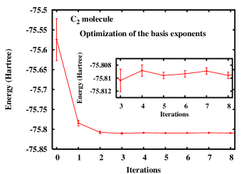
Figure 1: Convergence of the VMC total energy of the all-electron C₂ molecule during the optimization of the 12 exponent parameters in a wave function composed of a single Slater determinant multiplied by a Jastrow factor. Crude initial exponents have been intentionally chosen as the integers nearest to the exponent values of the CVB1 basis I. Ema, J. M. García de la Vega, G. Ramírez, R. López, J. F. Rico, H. Meissner and J. Paldus (2003). In this calculation, the number of MC sample was initially 10000 and this number was progressively increased at each iteration until a final statistical uncertainty of $0.5$ mHartree was reached.

Figure 1 shows the convergence of the VMC total energy of the all-electron C₂ molecule during the optimization of the 12 exponent parameters in a wave function composed of a Jastrow factor multiplied by a single Slater determinant where the Jastrow and orbital parameters have been previously optimized (with the exponents fixed at the CVB1 values). Crude initial exponents have been intentionally chosen as the integers nearest to the exponent values of the CVB1 basis. One sees that the linear energy minimization method yields a fast convergence of the energy in about three iterations, typically as fast as when optimizing the other parameters. The simultaneous optimization of the Jastrow, CSF, orbital and exponent parameters generally converges as fast as the simultaneous optimization of only the Jastrow, CSF and orbital parameters reported in Ref. Toulouse and Umrigar, 2007.

When optimizing the exponents without simultaneous optimization of the orbitals, we have found the optimization very stable, the introduction of the stabilization constant $a_{\text{diag}}$ often being unnecessary. However, when optimizing simultaneously the orbital and exponents parameters, the optimization tends to be less stable because of near redundancies between these two sets of parameters, and $a_{\text{diag}}$ typically increases up to $10^{-3}-10^{-4}$ to retain stability.

Tests on a few atoms have shown that, for the optimization of exponents only, the use of the orthonormalized basis functions of Eq. (9) tends to be a bit more stable. Typically, the overlap matrix $\overline{\mathbf{S}}$ of the wave function derivatives have eigenvalues that span about 7 orders of magnitude from $1$ to $10^{-7}$ for (unnormalized or normalized) nonorthogonalized functions whereas, for orthonormalized basis functions, the eigenvalues span only about 4 orders of magnitude from $1$ to $10^{-4}$. Thus, orthogonalization of the basis functions reduces the range of the eigenvalues, attenuating near redundancies among the exponent parameters. However, the wave function derivatives with respect to the exponents take significantly longer to compute when using orthonormalized basis functions, and in addition, when also optimizing the orbitals, the near redundancies between some orbital and exponents parameters make $a_{\text{diag}}$ increase anyway. Thus, we have not found it worthwhile for our purpose to use orthonormalized basis functions.

For the first-row atoms, optimizing the exponents (simultaneously with the other parameters) rather than using the exponents of the CVB1 basis typically yields improvements of the total VMC energies between 0.1 and 1 mHartree, which is at the edge of statistical significance and accuracy of the optimization. Thus, at the accuracy that we are concerned with, the exponents of the CVB1 basis for these atoms are nearly optimal for Jastrow-Slater wave functions. As expected, larger improvements are obtained for the first-row diatomic molecules. The largest improvement of the total energy is observed for the O₂ molecule with a gain of about $3.4$ mHartree in VMC and $1.2$ mHartree in DMC with a Jastrow-Slater single-determinant wave function. The largest improvement of the standard deviation of the energy is obtained for the Be₂ dimer using a Jastrow-Slater single-determinant wave function, with a gain of $0.25$ Hartree. (The standard deviation of the energy is $\sigma=0.57$ Hartree with the CVB1 exponents and $\sigma=0.32$ Hartree with the reoptimized exponents using pure energy minimization. A mixed minimization with an energy weighting of 0.95 and a variance weighting of 0.05 and reoptimized exponents results in the same energy but a $\sigma$ of 0.32, whereas a pure variance minimization yields a variational energy that is higher by 1 mHartree and a $\sigma$ of only 0.24.) Properties other than the energy might be more sensitive to the basis exponents. We note that the optimization method that we are using is designed to find local minima, and we cannot be sure that we have found the global minimum for the form of the trial wave function considered. In particular, optimization of the exponent parameters typically leads to multiple local minima. We have found that by optimizing the exponents it is possible to reduce the size of the basis, without sacrificing the energy or the energy variance, but the results in this paper were all obtained using a basis size corresponding to the CVB1 basis. A smaller basis has also the advantage of having fewer local minima.

As noted in Ref. Tachikawa et al., 1999, because the virial theorem within the Born-Oppenheimer approximation at the equilibrium nuclear geometry holds if the energy is stationary with respect to scaling of the electron coordinates, optimization of the basis exponents along with optimization of the scaling factors of the interelectron coordinates in the Jastrow factor permits one to satisfy exactly the virial theorem in VMC in the limit of infinite sample size.

V Potential energy curve of the C₂ molecule

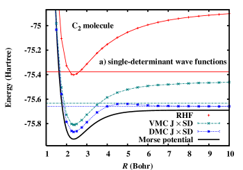
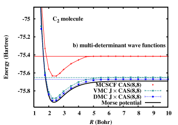
Figure 2: Total energy of the all-electron C₂ molecule as a function of the interatomic distance $R$ calculated in (plot a) RHF, VMC and DMC with a fully optimized Jastrow $\times$ single determinant wave function [J $\times$ SD], and (plot b) MCSCF CAS(8,8), VMC and DMC with a fully optimized Jastrow $\times$ multi-determinant CAS(8,8) wave function [J $\times$ CAS(8,8)], using the CVB1 Slater basis form I. Ema, J. M. García de la Vega, G. Ramírez, R. López, J. F. Rico, H. Meissner and J. Paldus (2003). In each case, the horizontal line represents twice the energy of an isolated atom calculated with the same method, and provides a check of the size consistency of the method. For comparison, a Morse potential Morse (1929) using accurate spectroscopic constants is also shown (see text).

Table 1: Distribution of the electrons among the two carbon atoms $A$ and $B$ of the C₂ molecule in the dissociation limit. For the neutral dissociations, only the distribution of the four $\pi$ electrons are considered since the remaining eight $\sigma$ electrons are unimportant for the study of the dissociation. The same methods used in Fig. 2 are compared. For the RHF and MCSCF wave functions, the percentages of the distributions can be calculated analytically.

	neutral dissociation			ionic dissociation
	$A(\uparrow\downarrow)+B(\uparrow\downarrow)$	$A(\uparrow\uparrow)+B(\downarrow\downarrow)$	$A(\downarrow\downarrow)+B(\uparrow\uparrow)$
RHF	25 %	6.25 %	6.25 %	62.5 %
VMC J$\times$SD	$\approx$ 43 %	$\approx$ 13 %	$\approx$ 13 %	$\approx$ 31 %
DMC J$\times$SD	$\approx$ 0 %	$\approx$ 50 %	$\approx$ 50 %	$\approx$ 0 %
MCSCF CAS(8,8)	33.33 %	33.33 %	33.33 %	0 %
VMC J$\times$CAS(8,8)	$\approx$ 33 %	$\approx$ 33 %	$\approx$ 33 %	$\approx$ 0 %
DMC J$\times$CAS(8,8)	$\approx$ 33 %	$\approx$ 33 %	$\approx$ 33 %	$\approx$ 0 %

In Fig. 2, we show the total energy curve of the all-electron C₂ molecule as a function of the interatomic distance $R$ calculated in (plot a) RHF, VMC and DMC with a fully optimized Jastrow $\times$ single-determinant wave function [J$\times$SD], and (plot b) MCSCF CAS(8,8), VMC and DMC with a fully optimized Jastrow $\times$ multi-determinant CAS(8,8) wave function [J$\times$CAS(8,8)]. In each case, the horizontal line represents twice the energy of an isolated atom calculated with the same method, and provides a check of the size consistency of the method. We stress that the wave functions have been optimized by energy minimization rather than variance minimization, and in appendix A we present an argument suggesting that, as regards size consistency, energy-optimized wave functions are to be preferred over variance-optimized wave functions. For comparison, we also plot a Morse potential Morse (1929), $E_{\text{Morse}}(R)=E_{\text{exact}}(R_{e})+D_{e}(1-e^{-x^{2}})^{2}$ where $x=2\beta(R-R_{e})/R_{e}$ and $\beta=\omega_{e}/(4\sqrt{B_{e}D_{e}})$, using an estimate of the exact energy at equilibrium $E_{\text{exact}}(R_{e})=-75.9265$ Hartree Bytautas and Ruedenberg (2005) and accurate spectroscopic constants: equilibrium distance $R_{e}=2.3481$ Filippi and Umrigar (1996), well-depth $D_{e}=6.44$ eV Bytautas and Ruedenberg (2005), first vibrational frequency $\omega_{e}=1855$ cm^-1 Linstrom and Mallard (June 2005) and rotational constant $B_{e}=1.81984$ cm^-1 Huber and Herzberg (1979). For analysis, we report in Table 1 the distribution of the four $\pi$ electrons among the two carbon atoms $A$ and $B$ in the dissociation limit, the remaining eight $\sigma$ electrons being unimportant for the study of the dissociation.

We note that Sorella et al. Sorella et al. (2007) have also reported recently QMC calculations of the potential energy curve of the C₂ molecule, using a pseudopotential and Jastrow antisymmetrized geminal power wave functions.

At very large interatomic distances, lack of ergodicity in the QMC calculations may be an issue, as electrons tend to remain stuck around an atom, and nonequilibrated results can be obtained. In VMC calculations it is always possible to make large moves of the electrons between the two atoms, as done for example in Ref. Sorella et al., 2007, but this is not possible in DMC calculations where dynamics of the moves is specified and becomes exact only in the small time-step limit. One can nevertheless avoid being deceived by using a large population of walkers (thereby improving the sampling of the configuration space), looking at the evolution of the results as the bond is stretched, and performing several runs with different starting locations of the walkers.

We first discuss the single-determinant case. RHF is of course not size consistent, and leads to a large percentage of incorrect ionic dissociations (62.5%). Our Jastrow factor has a multiplicatively separable form (at dissociation, it reduces to the product of the Jastrow factors employed for the isolated atoms), so that fulfillment of size consistency in VMC calculations is only dependent on the determinantal part of the wave function. The VMC calculation using a single determinant is not size consistent, but the Jastrow factor reduces the size-consistency error and decreases the percentage of ionic dissociations to about 31%. Interestingly, the DMC calculation using the nodes of a non-size-consistent single-determinant trial wave function appears to be size consistent within the accuracy of the calculation, ionic dissociations being absent. Moreover, examination of the distribution of electrons in the DMC calculation shows that the distribution $A(\uparrow\downarrow)+B(\uparrow\downarrow)$ has a vanishing probability in the dissociation limit (see Table 1). Only the distributions $A(\uparrow\uparrow)+B(\downarrow\downarrow)$ and $A(\downarrow\downarrow)+B(\uparrow\uparrow)$ remain at dissociation. In appendix B, we show that this implies that the singlet-spin symmetry of the ground-state is broken with an expectation value of the total spin operator $\hat{S}^{2}$ over the FN wave function of 2. In quantum chemistry, it is well known that spin (and/or spatial) symmetry breaking frequently occurs in unrestricted Hartree-Fock or unrestricted Kohn-Sham calculations at large interatomic distances where electron correlation gets stronger. Our results show that spin-symmetry breaking can also occur in DMC calculations even using an unbroken-symmetry trial wave function, meaning that its nodal surface does not impose the spin symmetry. One may wonder how the repeated application of a spin-independent Green function to an initial trial wave function that is a spin eigenstate (neglecting the small spin contamination that can be introduced by imposing spin-dependent electron-electron cusp conditions in the Jastrow factor Huang et al. (1998)) can result in a wave function that is not a spin eigenstate. In fact, breaking of spin symmetry is possible in DMC calculations because the Green function is not applied exactly but only by finite sampling. After all, the fermion-sign problem can also been seen as resulting from the breaking of the antisymmetry of the trial wave function due to finite sampling.

We now discuss the multi-determinant case. The MCSCF calculation in a full valence CAS, i.e. CAS(8,8) for the C₂ molecule, is size consistent, the corresponding atomic calculation being taken as a MCSCF CAS(4,4) calculation as in Refs. Toulouse and Umrigar, 2007 and Umrigar et al., 2007. Not surprisingly, the corresponding VMC and DMC calculations are also size consistent. The DMC energy curve agrees closely with the reference Morse potential. For these three calculations, at the dissociation limit, the distributions $A(\uparrow\downarrow)+B(\uparrow\downarrow)$, $A(\uparrow\uparrow)+B(\downarrow\downarrow)$ and $A(\downarrow\downarrow)+B(\uparrow\uparrow)$ are obtained with equal weights, which is expected for a proper spin-singlet wave function describing two dissociated carbon atoms, as noted in Ref. Sorella et al., 2007.

VI Results on first-row atoms and homonuclear diatomic molecules

Table 2: Total energies (in Hartree) and well depths (in eV) of first-row atoms and homonuclear diatomic molecules at their experimental bond lengths $R_{0}$ (in Bohr) using several computational methods (see text). The RHF and MCSCF calculations have been performed with the Slater CVB1 basis set I. Ema, J. M. García de la Vega, G. Ramírez, R. López, J. F. Rico, H. Meissner and J. Paldus (2003), expanding each Slater function into 14 Cartesian Gaussian functions. The QMC calculations have been performed with the true Slater basis set rather than its Gaussian expansion. The Jastrow, CSF, orbital and exponent parameters of the Jastrow-Slater wave functions have been optimized in VMC, and the resulting wave functions have been used in DMC. The DMC energies are for time step $\tau=0.01$ Hartree^-1, with the exception of Ne and Ne₂ for which the energies extrapolated to $\tau=0$ are given. The well depths have been calculated consistently using single-determinant (SD) wave functions for both the molecule and the atom, or, full valence complete active space (FVCAS) multi-determinant wave functions for both the molecule and the atom.

	Atoms
	Li (${}^{2}S$)	Be (${}^{1}S$)	B (${}^{2}P$)	C (${}^{3}P$)	N (${}^{4}S$)	O (${}^{3}P$)	F (${}^{2}P$)	Ne (${}^{1}S$)
	Numbers of CSFs in FVCAS wave functions
	1	2	2	2	1	1	1	1
	Total energies (Hartree)
RHF	-7.43271	-14.57299	-24.52903	-37.68849	-54.40060	-74.81065	-99.40937	-128.54556
MCSCF FVCAS		-14.61663	-24.56372	-37.70777
VMC J$\times$SD	-7.47793(5)	-14.64972(5)	-24.62936(5)	-37.81705(6)	-54.5628(1)	-75.0352(1)	-99.7003(1)	-128.9057(1)
VMC J$\times$FVCAS		-14.66668(5)	-24.64409(5)	-37.82607(5)
DMC J$\times$SD	-7.47805(1)	-14.65717(1)	-24.63990(2)	-37.82966(4)	-54.57587(4)	-75.05187(7)	-99.71827(5)	-128.92346(3)
DMC J$\times$FVCAS		-14.66727(1)	-24.64996(1)	-37.83620(1)
Estimated exact	-7.47806a	-14.66736a	-24.65391a	-37.8450a	-54.5892a	-75.0673a	-99.7339a	-128.9376a
	Molecules
	Li2 (${}^{1}\Sigma_{g}^{+}$)	Be2 (${}^{1}\Sigma_{g}^{+}$)	B2 (${}^{3}\Sigma_{g}^{-}$)	C2 (${}^{1}\Sigma_{g}^{+}$)	N2 (${}^{1}\Sigma_{g}^{+}$)	O2 (${}^{3}\Sigma_{g}^{-}$)	F2 (${}^{1}\Sigma_{g}^{+}$)	Ne2 (${}^{1}\Sigma_{g}^{+}$)
	Interatomic distances (Bohr)
	5.051b	4.65c	3.005d	2.3481d	2.075b	2.283b	2.668b	5.84g
	Numbers of CSFs in FVCAS wave functions
	8	38	137	165	107	30	8	1
	Total energies (Hartree)
RHF	-14.87127	-29.13148	-49.08961	-75.40154	-108.98650	-149.65881	-198.76323	-257.09105
MCSCF FVCAS	-14.89758	-29.22111	-49.22009	-75.63991	-109.13585	-149.76453	-198.84307
VMC J$\times$SD	-14.98255(5)	-29.29768(4)	-49.3457(5)	-75.8088(5)	-109.4520(5)	-150.2248(5)	-199.4209(5)	-257.80956(2)
VMC J$\times$FVCAS	-14.99229(5)	-29.33180(5)	-49.3916(2)	-75.8862(2)	-109.4851(3)	-150.2436(2)	-199.4443(3)
DMC J$\times$SD	-14.99167(2)	-29.31895(5)	-49.38264(9)	-75.8672(1)	-109.5039(1)	-150.2872(2)	-199.4861(2)	-257.84707(5)
DMC J$\times$FVCAS	-14.99456(1)	-29.33736(2)	-49.4067(2)	-75.9106(1)	-109.5206(1)	-150.29437(9)	-199.4970(1)
Estimated exact	-14.995(1)	-29.3380(4)	-49.415(2)	-75.9265f	-109.5427f	-150.3274f	-199.5304f	-257.8753
	Well depths (eV)
RHF	0.159	-0.395	0.858	0.668	5.042	1.021	-1.510	-0.00189
MCSCF FVCAS	0.875	-0.331	2.521	6.105	9.106	3.897	0.662
VMC J$\times$SD	0.726(3)	-0.048(3)	2.367(3)	4.75(1)	8.88(1)	4.20(1)	0.55(1)	-0.050(5)
VMC J$\times$FVCAS	0.991(3)	-0.042(3)	2.814(6)	6.369(6)	9.78(1)	4.713(8)	1.19(1)
DMC J$\times$SD	0.9679(8)	0.125(1)	2.798(3)	5.656(3)	9.583(3)	4.992(7)	1.349(6)	0.004(2)
DMC J$\times$FVCAS	1.0465(6)	0.0767(8)	2.906(3)	6.482(3)	10.037(3)	5.187(5)	1.645(4)
Estimated exact	1.06(4)c	0.09(1)c	2.92(6)e	6.44(2)f	9.908($<$3)f	5.241($<$3)f	1.693(5)f	0.00365g
a Ref. Chakravorty et al., 1993, b Ref. Huber and Herzberg, 1979, c Ref. Linstrom and Mallard, June 2005, d Ref. Filippi and Umrigar, 1996, e Ref. Langhoff and Bauschlicher, 1991, f Ref. Bytautas and Ruedenberg, 2005, g Ref. Aziz and Slaman, 1989.

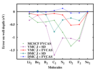
Figure 3: Error in well depths of the first-row homonuclear diatomic molecules using several computational methods (see text and Table 2).

In Table 2, we report total energies of the first-row atoms and homonuclear diatomic molecules at their experimental bond length using several computational methods: RHF, MCSCF in a full valence complete active space (FVCAS), VMC with Jastrow $\times$ single determinant [J$\times$SD] and Jastrow $\times$ multi-determinant FVCAS [J$\times$FVCAS] wave functions (where the Jastrow, CSF, orbital and exponent parameters have been simultaneously optimized), and DMC with the same J$\times$SD and J$\times$FVCAS wave functions. For atoms, the active space of FVCAS wave functions consists of the $2s$ and $2p$ orbitals. For the molecules, it consists of all the orbitals coming from the $n=2$ atomic shells, i.e. $2\sigma_{g}2\sigma_{u}3\sigma_{g}1\pi_{u,x}1\pi_{u,y}1\pi_{g,x}1\pi_{g,y}3\sigma_{u}$ (this is the energy ordering of the Hartree-Fock orbitals for 5 molecules out of the 8 molecules). For the atoms Li, N, O, F and Ne, and for the dimer Ne₂, orbital occupations and symmetry constraints imply that the FVCAS wave functions contain only a single determinant. Thus, for these systems, the FVCAS MCSCF wave functions are identical to the RHF wave functions, and the J$\times$FVCAS wave functions are identical to J$\times$SD wave functions. The well depths (dissociation energy + zero-point energy) have been calculated consistently by using single-determinant wave functions for both the molecule and the atom, or multi-determinant FVCAS wave functions for both the molecule and the atom. The errors of the computed well depths are plotted in Fig 3.

The largest errors of the DMC total energy using J$\times$FVCAS wave functions are obtained for the heaviest systems and are of the order of 15 mHartree for the atoms and 30 mHartree for the molecules. Of course, one can always improve the total energy by increasing the number of CSFs as done for example by Brown et al. Brown et al. (2007), but good well depths are already obtained with J$\times$FVCAS wave functions due to a compensation of errors between the atoms and the molecule. DMC calculations using J$\times$FVCAS wave functions give well depths with near chemical accuracy (1 kcal/mol $\approx$ 0.04 eV), the largest absolute error being of about 0.1 eV for the N₂ molecule. In particular, we note that, although the Be₂ dimer is unbound at the RHF, MCSCF and VMC level, the weak bond is well reproduced at the DMC level. Because of the extremely weak van der Waals bond of the Ne₂ dimer we computed the DMC energies of Ne and Ne₂ at four time steps $\tau=$ 0.020, 0.015, 0.010, and 0.005 Hartree^-1 and extrapolated to zero time step. The time-step error at $\tau=0.01$ for Ne₂ was $-0.0023$ Hartree whereas that for Ne was $-0.00068$ Hartree.

VII Conclusions

To summarize, we have extended our earlier published linear optimization method to allow for nonorthogonal orbitals. This then makes it possible to optimize all the parameters in the wave function, including the basis exponents. Moreover, by noting that the linear optimization method can be seen as an augmented Hessian method, we have shown that it is possible to minimize a linear combination of the energy and the energy variance with the linear optimization method. We have applied the method to the calculation of the full ground-state potential energy curve of the C₂ molecule, and we have shown that although a VMC calculation using a spin-restricted single-determinant Jastrow-Slater wave function is not size consistent, the corresponding DMC calculation using the same trial wave function is size consistent within statistical uncertainty. The price to pay for this size consistency is the breaking of the spin-singlet symmetry at dissociation: the fixed-node DMC wave function has an expectation value of $2$ for the total spin operator $\hat{S}^{2}$, although the spin-singlet trial wave function is an eigenstate of $\hat{S}^{2}$ with eigenvalue $0$. Of course, using multi-determinant FVCAS Jastrow-Slater wave functions, both the VMC and the DMC calculations are size consistent without breaking of spin symmetry. Finally, we have performed calculations on the first-row atoms and homonuclear diatomic molecules and showed that well depths can be computed with near chemical accuracy using just fully optimized multi-determinant FVCAS Jastrow-Slater wave functions.

Appendix A A remark on size consistency and variance minimization

In this appendix, we briefly review the concept of size consistency of an electronic-structure method (see, e.g., Refs. Duch and Diercksen, 1994; Helgaker et al., 2002; Nooijen et al., 2005 for more details), and we give an argument for preferring energy-optimized wave functions over variance-optimized wave functions as regards size consistency.

A.1 Definition of size consistency

Consider an electronic system $AB$ made of two noninteracting fragments $A$ and $B$ (e.g., a diatomic molecule at dissociation). This system has a Hamiltonian

$$\hat{H}_{AB}=\hat{H}_{A}+\hat{H}_{B},$$ (92)

where $\hat{H}_{A}$ and $\hat{H}_{B}$ are the Hamiltonians of the fragments, commuting with each other. If $E_{A}$ and $E_{B}$ are the (approximate) energies of the fragments given by some method, and $E_{AB}$ is the (approximate) energy of the composite system given by the same method, then this method is said to be size consistent if and only if

$$E_{AB}=E_{A}+E_{B},$$ (93)

i.e., the energy is additive.

In particular, if $|A\rangle=\hat{\psi}_{A}|\text{vac}\rangle$ and $|B\rangle=\hat{\psi}_{B}|\text{vac}\rangle$ are the (approximate) wave functions given by the method under consideration where $\hat{\psi}_{A}$ and $\hat{\psi}_{B}$ are second-quantized wave operators (commuting or anticommuting with each other), then a sufficient condition for size consistency of the method is that it leads to an (approximate) wave function for the composite system of the product form

$$|AB\rangle_{P}=\hat{\psi}_{A}\hat{\psi}_{B}|\text{vac}\rangle,$$ (94)

i.e., the wave function is multiplicatively separable. However, this is not a necessary condition, as exemplified by perturbation theory (see, e.g., the discussion in Ref. Nooijen et al., 2005). Also, in general, due to the nonlocality of the total spin operator $\hat{S}^{2}$, one has in fact to consider a sum of products of degenerate spin-multiplet component wave functions of the fragments to accommodate non-singlet spin symmetry, but it is sufficient to take the simple product form of Eq. (94) for our purpose. If the wave function of the system $AB$ has this product form, then it is easy to show that the energy variance is also additively separable

$$V_{AB}=V_{A}+V_{B},$$ (95)

where $V_{AB}=\langle AB|(\hat{H}_{AB}-E_{AB})^{2}|AB\rangle/\langle AB|AB\rangle$ is the energy variance of the system $AB$, and $V_{A}=\langle A|(\hat{H}_{A}-E_{A})^{2}|A\rangle/\langle A|A\rangle$ and $V_{B}=\langle B|(\hat{H}_{B}-E_{B})^{2}|B\rangle/\langle B|B\rangle$ are the energy variances of the fragments.

A.2 Multiplicative separability of energy-optimized linear wave functions

Before discussing variance-optimized wave functions, it is useful to repeat briefly the proof of the multiplicative separability of energy-optimized linear wave functions, given for instance in Ref. Helgaker et al., 2002.

Consider that the fragments are described by the following linearly parametrized (approximate) wave functions

$$|A\rangle=\sum_{i}c_{iA}|i_{A}\rangle,$$ (96a)

and

$$|B\rangle=\sum_{j}c_{jB}|j_{B}\rangle,$$ (96b)

where $|i_{A}\rangle=\hat{\psi}_{iA}|\text{vac}\rangle$ and $|j_{B}\rangle=\hat{\psi}_{jB}|\text{vac}\rangle$ are some many-body basis states, and the coefficients $c_{iA}$ and $c_{jB}$ are determined by requiring the stationarity of the energy of each fragment

$$\frac{\partial E_{A}}{\partial c_{iA}}=2\,\frac{\langle i_{A}|\hat{H}_{A}-E_{A}|A\rangle}{\langle A|A\rangle}=0,$$ (97a)

$$\frac{\partial E_{B}}{\partial c_{jB}}=2\,\frac{\langle j_{B}|\hat{H}_{B}-E_{B}|B\rangle}{\langle B|B\rangle}=0.$$ (97b)

Correspondingly, consider that the composite system is described by a linearly parametrized wave function in the product basis $|i_{A}j_{B}\rangle=\hat{\psi}_{iA}\hat{\psi}_{jB}|\text{vac}\rangle$

$$|AB\rangle=\sum_{ij}c_{ij}|i_{A}j_{B}\rangle,$$ (98)

where the coefficients $c_{ij}$ are also consistently determined by imposing the stationarity of the energy

$$\frac{\partial E_{AB}}{\partial c_{ij}}=2\,\frac{\langle i_{A}j_{B}|\hat{H}_{AB}-E_{AB}|AB\rangle}{\langle AB|AB\rangle}=0.$$ (99)

It is then easy to see that the product wave function $|AB\rangle_{P}=\hat{\psi}_{A}\hat{\psi}_{B}|\text{vac}\rangle$ makes the corresponding energy $E_{AB}^{P}$ stationary

$$\frac{\partial E_{AB}^{P}}{\partial c_{ij}} = 2\,\frac{\langle i_{A}|\hat{H}_{A}-E_{A}|A\rangle}{\langle A|A\rangle}\,\frac{\langle j_{B}|B\rangle}{\langle B|B\rangle}$$ (100)

$$+\,2\,\frac{\langle j_{B}|\hat{H}_{B}-E_{B}|B\rangle}{\langle B|B\rangle}\,\frac{\langle i_{A}|A\rangle}{\langle A|A\rangle}=0,$$

since both terms vanish according to Eqs. (97b). The product wave function is thus a possible solution, and, if this is the actual solution given by the method, then the method is size consistent.

As an aside, we note that the energy of the product wave function will converge exponentially to the sum of the constituent energies as a function of the interfragment distance because the overlap of the fragment wave functions decays exponentially. On the other hand, the true wave function has an energy that converges only as an inverse power to the sum of the constituent energies (Van der Waals interaction).

A.3 Lack of multiplicative separability of variance-optimized linear wave functions

In the case of variance-optimized linear wave functions, the coefficients $c_{iA}$ and $c_{jB}$ of the fragment wave functions of Eq. (96b) are determined by requiring the stationarity of the energy variance

$$\frac{\partial V_{A}}{\partial c_{iA}}=2\,\frac{\langle i_{A}|(\hat{H}_{A}-E_{A})^{2}-V_{A}|A\rangle}{\langle A|A\rangle}=0,$$ (101a)

$$\frac{\partial V_{B}}{\partial c_{jB}}=2\,\frac{\langle j_{B}|(\hat{H}_{B}-E_{B})^{2}-V_{B}|B\rangle}{\langle B|B\rangle}=0.$$ (101b)

Correspondingly, the coefficients $c_{ij}$ of the composite wave function of Eq. (98) are also determined by imposing stationarity of the energy variance

$$\frac{\partial V_{AB}}{\partial c_{ij}}=2\,\frac{\langle i_{A}j_{B}|(\hat{H}_{AB}-E_{AB})^{2}-V_{AB}|AB\rangle}{\langle AB|AB\rangle}=0.$$ (102)

In contrast to the case of energy-optimized wave functions, the product wave function $|AB\rangle_{P}=\hat{\psi}_{A}\hat{\psi}_{B}|\text{vac}\rangle$ now does not make the corresponding energy variance $V_{AB}^{P}$ stationary

$$\frac{\partial V_{AB}^{P}}{\partial c_{ij}} = 2\,\frac{\langle i_{A}|(\hat{H}_{A}-E_{A})^{2}-V_{A}|A\rangle}{\langle A|A\rangle}\,\frac{\langle j_{B}|B\rangle}{\langle B|B\rangle}$$ (103)

$$+\,2\,\frac{\langle j_{B}|(\hat{H}_{B}-E_{B})^{2}-V_{B}|B\rangle}{\langle B|B\rangle}\,\frac{\langle i_{A}|A\rangle}{\langle A|A\rangle}$$

$$+\,4\,\frac{\langle i_{A}|\hat{H}_{A}-E_{A}|A\rangle}{\langle A|A\rangle}\,\frac{\langle j_{B}|\hat{H}_{B}-E_{B}|B\rangle}{\langle B|B\rangle}$$

$$\not=0,$$

since the last term in Eq. (103) is the product of the energy gradients of the fragments which do not now generally vanish. Thus, the wave function minimizing the energy variance of the composite system is not a product wave function. This suggests that variance minimization does not generally yield additively separable energies, $E_{AB}\not=E_{A}+E_{B}$. Further, since the variance is additive for the product wave function, if the method minimizes over a space that includes the product wave function, then $V_{AB}\leq V_{A}+V_{B}$. This happens by having anticorrelated energy fluctuations on the two fragments. Of course, in the limit of exact wave functions, the gradients of the energy and of the energy variance simultaneously vanish, and size consistency is ensured. Consequently, the magnitude of the violation of size consistency of variance-optimized linear wave functions is expected to become smaller as the wave function becomes more accurate.

Appendix B Spin-symmetry breaking in DMC for the C₂ molecule at dissociation

In this appendix, we show how the information on the real-space location of the electrons in DMC calculations of the C₂ molecule at dissociation using a spin-restricted single-determinant trial wave function reveals that the spin-singlet symmetry of the exact ground state is broken in the FN wave function.

For that, we need to determine the expectation value of the total spin operator $\hat{S}^{2}$ over the FN wave function. As we use in the QMC calculation a real-space spin-assigned wave function, we first need to reconstitute the corresponding total wave function. Reference Huang et al., 1998 shows how to do so using straightforward first quantization. Here, we use the alternative formalism of real-space second quantization.

In this formalism, the total wave function $|\Gamma\rangle$ in abstract Hilbert space corresponding to a $N$-electron real-space spin-assigned wave function $\Psi(\mathbf{r}_{1},\mathbf{r}_{2},\cdots,\mathbf{r}_{N})=\langle\mathbf{r}_{1}\uparrow,\mathbf{r}_{2}\uparrow,\cdots,\mathbf{r}_{N}\downarrow|\Psi\rangle$ with $N_{\uparrow}$ spin-up followed by $N_{\downarrow}$ spin-down electrons is written as

$$|\Gamma\rangle=\frac{1}{\sqrt{N_{\uparrow}!N_{\downarrow}!}}\int d\mathbf{r}_{1}d\mathbf{r}_{2}\cdots d\mathbf{r}_{N}\,\Psi(\mathbf{r}_{1},\mathbf{r}_{2},\cdots,\mathbf{r}_{N})$$

$$\hat{\psi}^{\dagger}_{\uparrow}(\mathbf{r}_{1})\hat{\psi}^{\dagger}_{\uparrow}(\mathbf{r}_{2})\cdots\hat{\psi}^{\dagger}_{\downarrow}(\mathbf{r}_{N})|\text{vac}\rangle,\,\,\,$$ (104)

where $\hat{\psi}^{\dagger}_{\sigma}(\mathbf{r})$ is the fermionic field creation operator at point $\mathbf{r}$ and spin $\sigma$. In Eq. (104), $\Psi(\mathbf{r}_{1},\mathbf{r}_{2},\cdots,\mathbf{r}_{N})$ is taken as antisymmetric under the exchange of two same-spin electron space coordinates and normalized to unity, i.e. $\int d\mathbf{r}_{1}d\mathbf{r}_{2}\cdots d\mathbf{r}_{N}|\Psi(\mathbf{r}_{1},\mathbf{r}_{2},\cdots,\mathbf{r}_{N})|^{2}=1$, implying that $|\Gamma\rangle$ is also normalized to unity, $\langle\Gamma|\Gamma\rangle=1$. Even if the wave function $|\Psi\rangle$ is not antisymmetric under the exchange of two opposite-spin electrons (product of spin-up and spin-down determinants), the total wave function $|\Gamma\rangle$ is always fully antisymmetric.

To study the dissociation of the C₂ molecule, it is sufficient to consider only the four $\pi$ electrons. The total FN wave function $|\Gamma_{\text{FN}}\rangle$ corresponding to the spin-assigned real-space FN wave function $\Psi_{\text{FN}}(\mathbf{r}_{1},\mathbf{r}_{2},\mathbf{r}_{3},\mathbf{r}_{4})$ is thus written as

$$|\Gamma_{\text{FN}}\rangle=\frac{1}{2}\int d\mathbf{r}_{1}d\mathbf{r}_{2}d\mathbf{r}_{3}d\mathbf{r}_{4}\Psi_{\text{FN}}(\mathbf{r}_{1},\mathbf{r}_{2},\mathbf{r}_{3},\mathbf{r}_{4})$$

$$\hat{\psi}^{\dagger}_{\uparrow}(\mathbf{r}_{1})\hat{\psi}^{\dagger}_{\uparrow}(\mathbf{r}_{2})\hat{\psi}^{\dagger}_{\downarrow}(\mathbf{r}_{3})\hat{\psi}^{\dagger}_{\downarrow}(\mathbf{r}_{4})|\text{vac}\rangle,$$ (105)

with the antisymmetry constraints

$$\Psi_{\text{FN}}(\mathbf{r}_{2},\mathbf{r}_{1},\mathbf{r}_{3},\mathbf{r}_{4})=-\Psi_{\text{FN}}(\mathbf{r}_{1},\mathbf{r}_{2},\mathbf{r}_{3},\mathbf{r}_{4}),$$ (106a)

$$\Psi_{\text{FN}}(\mathbf{r}_{1},\mathbf{r}_{2},\mathbf{r}_{4},\mathbf{r}_{3})=-\Psi_{\text{FN}}(\mathbf{r}_{1},\mathbf{r}_{2},\mathbf{r}_{3},\mathbf{r}_{4}).$$ (106b)

Examination of the real-space location of the electrons during DMC calculations using a spin-restricted single-determinant trial wave function shows that, in the dissociation limit, the mixed distribution $\Psi(\mathbf{r}_{1},\mathbf{r}_{2},\mathbf{r}_{3},\mathbf{r}_{4})\Psi_{\text{FN}}(\mathbf{r}_{1},\mathbf{r}_{2},\mathbf{r}_{3},\mathbf{r}_{4})$ vanishes whenever two electrons of opposite spins are in the neighborhood of the same C nucleus. In contrast, we know from VMC calculations that the trial wave function $\Psi(\mathbf{r}_{1},\mathbf{r}_{2},\mathbf{r}_{3},\mathbf{r}_{4})$ does not forbid dissociation with two opposite-spin electrons around the same nucleus, thus we conclude that it is the FN wave function $\Psi_{\text{FN}}(\mathbf{r}_{1},\mathbf{r}_{2},\mathbf{r}_{3},\mathbf{r}_{4})$ that vanishes for this type of dissociation. In other words, it means that at dissociation $\Psi_{\text{FN}}(\mathbf{r}_{1},\mathbf{r}_{2},\mathbf{r}_{4},\mathbf{r}_{3})$ can be written as (assuming that inversion symmetry is preserved)

$$\Psi_{\text{FN}}(\mathbf{r}_{1},\mathbf{r}_{2},\mathbf{r}_{4},\mathbf{r}_{3}) = f_{A}(\mathbf{r}_{1},\mathbf{r}_{2})g_{B}(\mathbf{r}_{3},\mathbf{r}_{4})$$ (107)

$$+g_{B}(\mathbf{r}_{1},\mathbf{r}_{2})f_{A}(\mathbf{r}_{3},\mathbf{r}_{4}),$$

where $f_{A}$ and $g_{B}$ are antisymmetric two-electron functions localized around nuclei $A$ and $B$, respectively.

We now investigate the spin symmetry of this FN wave function. First, using the anticommutation rules of the field operators, it is easy to show that the wave function $|\Gamma_{\text{FN}}\rangle$ is an eigenstate of the spin-projection operator $\hat{S}_{z}=(1/2)\int d\mathbf{r}[\hat{\psi}^{\dagger}_{\uparrow}(\mathbf{r})\hat{\psi}_{\uparrow}(\mathbf{r})-\hat{\psi}^{\dagger}_{\downarrow}(\mathbf{r})\hat{\psi}_{\downarrow}(\mathbf{r})]$ with eigenvalue zero

$$\hat{S}_{z}|\Gamma_{\text{FN}}\rangle=0,$$ (108)

for any function $\Psi_{\text{FN}}(\mathbf{r}_{1},\mathbf{r}_{2},\mathbf{r}_{4},\mathbf{r}_{3})$. The action of the total spin operator $\hat{S}^{2}=\hat{S}_{+}\hat{S}_{-}+\hat{S}_{z}(\hat{S}_{z}-1)$ with $\hat{S}_{+}=\int d\mathbf{r}\,\hat{\psi}^{\dagger}_{\uparrow}(\mathbf{r})\hat{\psi}_{\downarrow}(\mathbf{r})$ and $\hat{S}_{-}=\int d\mathbf{r}\,\hat{\psi}^{\dagger}_{\downarrow}(\mathbf{r})\hat{\psi}_{\uparrow}(\mathbf{r})$ on $|\Gamma_{\text{FN}}\rangle$ gives

$$\hat{S}^{2}|\Gamma_{\text{FN}}\rangle=\frac{1}{2}\int d\mathbf{r}_{1}d\mathbf{r}_{2}d\mathbf{r}_{3}d\mathbf{r}_{4}[2\Psi_{\text{FN}}(\mathbf{r}_{1},\mathbf{r}_{2},\mathbf{r}_{3},\mathbf{r}_{4})$$

$$-4\Psi_{\text{FN}}(\mathbf{r}_{1},\mathbf{r}_{3},\mathbf{r}_{2},\mathbf{r}_{4})]\hat{\psi}^{\dagger}_{\uparrow}(\mathbf{r}_{1})\hat{\psi}^{\dagger}_{\uparrow}(\mathbf{r}_{2})\hat{\psi}^{\dagger}_{\downarrow}(\mathbf{r}_{3})\hat{\psi}^{\dagger}_{\downarrow}(\mathbf{r}_{4})|\text{vac}\rangle,\,\,\,\,\,$$ (109)

where the anticommutation rules of the field operators and permutations of electron space coordinates have been used. Equation (109) shows that $|\Gamma_{\text{FN}}\rangle$ is generally not an eigenstate of $\hat{S}^{2}$. At dissociation, it is nevertheless possible to calculate the expectation value of $\hat{S}^{2}$ over $|\Gamma_{\text{FN}}\rangle$

$$\langle\Gamma_{\text{FN}}|\hat{S}^{2}|\Gamma_{\text{FN}}\rangle = 2-\int d\mathbf{r}_{1}d\mathbf{r}_{2}d\mathbf{r}_{3}d\mathbf{r}_{4}\Psi_{\text{FN}}(\mathbf{r}_{1},\mathbf{r}_{2},\mathbf{r}_{3},\mathbf{r}_{4})$$ (110)

$$\times\Psi_{\text{FN}}(\mathbf{r}_{1},\mathbf{r}_{3},\mathbf{r}_{2},\mathbf{r}_{4})$$

$$= 2,$$

since the last integral vanishes due to the localized form of $\Psi_{\text{FN}}(\mathbf{r}_{1},\mathbf{r}_{3},\mathbf{r}_{2},\mathbf{r}_{4})$ given in Eq. (107).

In conclusion, we have shown that the singlet-spin symmetry of the ground-state of the C₂ molecule is broken in the FN wave function at dissociation using the nodes of a spin-restricted single-determinant wave function. The expectation value of $\hat{S}^{2}$ over the FN wave function is $2$, which is identical to the value found for the lowest broken symmetry solution of the unrestricted Hartree-Fock Lepetit et al. (1989) or unrestricted Kohn-Sham equations with usual approximate density functionals Goursot et al. (1995).

References

- Hammond et al. (1994) B. L. Hammond, J. W. A. Lester, and P. J. Reynolds, Monte Carlo Methods in Ab Initio Quantum Chemistry (World Scientific, Singapore, 1994).
- Nightingale and Umrigar (1999) M. P. Nightingale and C. J. Umrigar, eds., Quantum Monte Carlo Methods in Physics and Chemistry, NATO ASI Ser. C 525 (Kluwer, Dordrecht, 1999).
- Foulkes et al. (2001) W. M. C. Foulkes, L. Mitas, R. J. Needs, and G. Rajagopal, Rev. Mod. Phys. 73, 33 (2001).
- Toulouse and Umrigar (2007) J. Toulouse and C. J. Umrigar, J. Chem. Phys. 126, 084102 (2007).
- Umrigar et al. (2007) C. J. Umrigar, J. Toulouse, C. Filippi, S. Sorella, and R. G. Hennig, Phys. Rev. Lett. 98, 110201 (2007).
- Nightingale and Melik-Alaverdian (2001) M. P. Nightingale and V. Melik-Alaverdian, Phys. Rev. Lett. 87, 043401 (2001).
- Toulouse et al. (2007) J. Toulouse, R. Assaraf, and C. J. Umrigar, J. Chem. Phys. 126, 244112 (2007).
- Brown et al. (2007) M. D. Brown, J. R. Trail, P. L. Ríos, and R. J. Needs, J. Chem. Phys. 126, 224110 (2007).
- Tachikawa et al. (1998) M. Tachikawa, K. Mori, K. Suzuki, and K. Iguchi, Int. J. Quantum Chem. 70, 491 (1998).
- Tachikawa et al. (1999) M. Tachikawa, K. Taneda, and K. Mori, Int. J. Quantum Chem. 75, 497 (1999).
- Tachikawa and Osamura (2000) M. Tachikawa and Y. Osamura, J. Chem. Phys. 113, 4942 (2000).
- Umrigar and Filippi (2005) C. J. Umrigar and C. Filippi, Phys. Rev. Lett. 94, 150201 (2005).
- (13) C. J. Umrigar, unpublished.
- Filippi and Umrigar (1996) C. Filippi and C. J. Umrigar, J. Chem. Phys. 105, 213 (1996).
- Güçlü et al. (2005) A. D. Güçlü, G. S. Jeon, C. J. Umrigar, and J. K. Jain, Phys. Rev. B 72, 205327 (2005).
- Kato (1957) T. Kato, Comm. Pure Appl. Math. 10, 151 (1957).
- van Lenthe and Balint-Kurti (1983) J. H. van Lenthe and G. G. Balint-Kurti, J. Chem. Phys. 78, 5699 (1983).
- van Lenthe et al. (1991) J. H. van Lenthe, J. Verbeek, and P. Pulay, Mol. Phys. 73, 1159 (1991).
- Cooper (2002) D. L. Cooper, ed., Valence Bond Theory (Elsevier, 2002).
- Helgaker et al. (2002) T. Helgaker, P. Jørgensen, and J. Olsen, Molecular Electronic-Structure Theory (Wiley, Chichester, 2002).
- Roos et al. (1980) B. O. Roos, P. R. Taylor, and P. E. M. Siegbahn, Chem. Phys. 48, 157 (1980).
- Löwdin (1950) P.-O. Löwdin, J. Chem. Phys. 18, 365 (1950).
- Löwdin (1956) P.-O. Löwdin, Adv. Phys. 5, 1 (1956).
- Jørgensen and Simons (1983) P. Jørgensen and J. Simons, J. Chem. Phys. 79, 334 (1983).
- Levy and Berthier (1968) B. Levy and G. Berthier, Int. J. Quantum Chem. 2, 307 (1968).
- Grein and Chang (1971) F. Grein and T. C. Chang, Chem. Phys. Lett. 12, 44 (1971).
- Chang and Grein (1972) T. C. Chang and F. Grein, J. Chem. Phys. 57, 5270 (1972).
- Banerjee and Grein (1976) A. Banerjee and F. Grein, Int. J. Quantum Chem. 10, 123 (1976).
- B. H. Lengsfield III (1980) B. H. Lengsfield III, J. Chem. Phys. 73, 382 (1980).
- Yarkony (1981) D. R. Yarkony, Chem. Phys. Lett. 77, 634 (1981).
- B. H. Lengsfield III and B. liu (1981) B. H. Lengsfield III and B. liu, J. Chem. Phys. 75, 478 (1981).
- Shepard et al. (1982) R. Shepard, I. Shavitt, and J. Simons, J. Chem. Phys. 76, 543 (1982).
- Jensen and Jørgensen (1984) H. J. A. Jensen and P. Jørgensen, J. Chem. Phys. 80, 1204 (1984).
- Banerjee et al. (1985) A. Banerjee, N. Adams, J. Simons, and R. Shepard, J. Phys. Chem. 89, 52 (1985).
- Baker (1986) J. Baker, J. Comput. Chem. 7, 385 (1986).
- Khait et al. (1995) Y. G. Khait, A. I. Panin, and A. S. Averyanov, Int. J. Quantum Chem. 54, 329 (1995).
- Anglada and Bofill (1997) J. M. Anglada and J. M. Bofill, Int. J. Quantum Chem. 62, 153 (1997).
- Eckert et al. (1997) F. Eckert, P. Pulay, and H.-J. Werner, J. Comput. Chem. 18, 1473 (1997).
- Ceperley (1986) D. M. Ceperley, J. Stat. Phys. 43, 815 (1986).
- Ma et al. (2005) A. Ma, N. D. Drummond, M. D. Towler, and R. J. Needs, Phys. Rev. E 71, 066704 (2005).
- Sorella (2005) S. Sorella, Phys. Rev. B 71, 241103 (2005).
- Schmidt et al. (1993) M. W. Schmidt, K. K. Baldridge, J. A. Boatz, S. T. Elbert, M. S. Gordon, J. H. Jensen, S. Koseki, N. Matsunaga, K. A. Nguyen, S. J. Su, et al., J. Comput. Chem. 14, 1347 (1993).
- I. Ema, J. M. García de la Vega, G. Ramírez, R. López, J. F. Rico, H. Meissner and J. Paldus (2003) I. Ema, J. M. García de la Vega, G. Ramírez, R. López, J. F. Rico, H. Meissner and J. Paldus, J. Comput. Chem. 24, 859 (2003).
- Hehre et al. (1969) W. J. Hehre, R. F. Stewart, and J. A. Pople, J. Chem. Phys. 51, 2657 (1969).
- Stewart (1970) R. F. Stewart, J. Chem. Phys. 52, 431 (1970).
- (46) A. Kollias, P. Reinhardt, and R. Assaraf, in preparation. A variety of Slater basis functions along with STO-NG expansions are available at the following website: http://www.slaterbasissetlibrary.net/.
- (47) CHAMP, a quantum Monte Carlo program written by C. J. Umrigar, C. Filippi and Julien Toulouse, URL http://www.ccmr.cornell.edu/~cyrus/champ.html.
- Umrigar (1993) C. J. Umrigar, Phys. Rev. Lett. 71, 408 (1993).
- Umrigar (1999) C. J. Umrigar, in Quantum Monte Carlo Methods in Physics and Chemistry, edited by M. P. Nightingale and C. J. Umrigar (Kluwer, Dordrecht, 1999), NATO ASI Ser. C 525, p. 129.
- Grimm and Storer (1971) R. Grimm and R. G. Storer, J. Comput. Phys. 7, 134 (1971).
- Anderson (1975) J. B. Anderson, J. Chem. Phys. 63, 1499 (1975).
- Anderson (1976) J. B. Anderson, J. Chem. Phys. 65, 4121 (1976).
- Reynolds et al. (1982) P. J. Reynolds, D. M. Ceperley, B. J. Alder, and W. A. Lester, J. Chem. Phys. 77, 5593 (1982).
- Moskowitz et al. (1982) J. W. Moskowitz, K. E. Schmidt, M. A. Lee, and M. H. Kalos, J. Chem. Phys. 77, 349 (1982).
- Umrigar et al. (1993) C. J. Umrigar, M. P. Nightingale, and K. J. Runge, J. Chem. Phys. 99, 2865 (1993).
- Morse (1929) P. M. Morse, Phys. Rev. 34, 57 (1929).
- Bytautas and Ruedenberg (2005) L. Bytautas and K. Ruedenberg, J. Chem. Phys. 122, 154110 (2005).
- Linstrom and Mallard (June 2005) P. J. Linstrom and W. G. Mallard, eds., NIST Chemistry WebBook, NIST Standard Reference Database Number 69 (June 2005).
- Huber and Herzberg (1979) K. P. Huber and G. Herzberg, Molecular Spectra and Molecular Structure - IV. Constants of Diatomic Molecules (van Nostrand Reinhold Company, 1979).
- Sorella et al. (2007) S. Sorella, M. Casuala, and D. Rocca, J. Chem. Phys. 127, 014105 (2007).
- Huang et al. (1998) C.-J. Huang, C. Filippi, and C. J. Umrigar, J. Chem. Phys. 108, 8838 (1998).
- Chakravorty et al. (1993) S. J. Chakravorty, S. R. Gwaltney, E. R. Davidson, F. A. Parpia, and C. F. Fischer, Phys. Rev. A 47, 3649 (1993).
- Langhoff and Bauschlicher (1991) S. R. Langhoff and C. W. Bauschlicher, J. Chem. Phys. 95, 5882 (1991).
- Aziz and Slaman (1989) R. A. Aziz and M. J. Slaman, Chem. Phys. 130, 187 (1989).
- Duch and Diercksen (1994) W. Duch and G. H. F. Diercksen, J. Chem. Phys. 101, 3018 (1994).
- Nooijen et al. (2005) M. Nooijen, K. R. Shamasundary, and D. Mukherjee, Mol. Phys. 103, 2277 (2005).
- Lepetit et al. (1989) M. B. Lepetit, J. P. Malrieu, and M. Pelissier, Phys. Rev. A 39, 981 (1989).
- Goursot et al. (1995) A. Goursot, J. P. Malrieu, and D. R. Salahub, Theor. Chim. Acta 91, 225 (1995).