Static charged fluid around a massive magnetic dipole

Abstract

An analytical solution of Einstein-Maxwell equations with a static fluid as a source is presented. The spacetime is represented by the axially symmetric Weyl metric and the energy-momentum tensor describes a coupling of a fluid with an electromagnetic field. When appropriate limits are performed we recover the well-known solutions of Gutsunaev-Manko and Schwarzschild. Also, using Eckart’s thermodynamics, we calculated the temperature, the mechanical pressure, the charge density and the energy density of the system. The analysis of thermodynamic quantities suggests that the solution can be used to represent a magnetized compact stellar object surrounded by a charged fluid.

I Introduction

The study of magnetic fields in astrophysical objects such as white dwarfs, neutron stars, pulsars and black holes, has grown sharply in recent years akm:pan ; fuk:war ; sot:col ; agu:pon ; kun . In fact, several observations show that there are various scenarios where the magnetic fields and general relativity can not be neglected . One of them is the presence of strong magnetic fields in active galactic nuclei lob ; aha ; zak:etal ; gre:etal . These nuclei are known to produce more radiation than the rest of the entire galaxy and directly affect its structure and evolution. Another scenario is the production of relativistic collimated jets in the inner regions of accretion discs, which can be explained considering magneto-centrifugal mechanisms liu:sha ; aki:whe ; mku ; jet ; ust:kol ; kra:li . Also, magnetic fields are important in understanding the interplay between magnetic and thermal processes for strongly magnetic neutron stars agu:pon ; hen:fro ; med:lai . At least $10\%$ of all neutron stars are born as magnetars, with magnetic fields above $10^{14}$ G li:van ; pav:bez ; ibr:swa . Analytical models that describe these astrophysical objects are often associated with solutions of Einstein’s equations sch1 ; sch2 ; ker ; newman ; Rei ; nor . In the context of relativistic hydrostatic models, the Tolman-Oppenheimer-Volkov tolman ; oppi equations describe the internal structure of general relativistic static perfect fluid spheres, e.g. neutron stars. In the search for more realistic models for compact stellar systems, the energy-momentum tensor, the source of Einstein’s equations, is modified by introducing more complex terms that take into account additional physical properties as, for example, electromagnetic fields. In the case of relativistic magneto-hydrodynamics the reduction of this non-linear system leads often to simple models with limited applicability. For this reason, they are frequently superseded by numerical models BHsim ; GUZ ; font . Despite of this complexity, sometimes we can have useful analytical solutions, e.g., the Gutsunaev-Manko solution that describes the gravitational field of one static massive magnetic dipole gus . The aim of this work is to construct an analytical solution to the Einstein-Maxwell field equations coupled with a fluid in order to represent a static configuration that can be used to characterize the gravitational field of a magnetized astrophysical object surrounded by a charged fluid.

The article is organized as follows. In Sec. II we present the Einstein equations and the energy-momentum tensor to be considered. In Sec. III, we exhibit the solution of the Einstein equations. In Sec. IV we study the thermodynamical properties of the system. Finally, in Sec. V, we summarize our results.

II Coupling of fields

The spacetime for our model is represented by the Weyl metric,

$$ds^{2}=f^{-1}\left(e^{2\Lambda}\left[d\rho^{2}+dz^{2}\right]+\rho^{2}d\varphi^{2}\right)-fdt^{2},$$ (1)

where $f=f(\rho,z)$ and $\Lambda=\Lambda(\rho,z)$. The coordinate range are the usual for axial symmetry. Our conventions are: $G=c=1$, metric signature +2, partial and covariant derivatives with respect to the coordinate $x_{\mu}$ denoted by $,\mu$ and $;\mu$, respectively. Greek indices run from 1 to 4, with $(1,2,3,4)=(\rho,z,\varphi,t)$, and Latin indices run from 1 to 3. The aim of this work is to solve Einstein’s equations with an energy-momentum tensor representing the coupling between a fluid and an electromagnetic field. Thus, in our model, the energy-momentum tensor is the sum of the electromagnetic energy-momentum tensor and a fluid energy-momentum tensor. The electromagnetic energy-momentum tensor considered is

$$\overset{(EM)}{T_{\alpha\beta}}=\frac{1}{4\pi}\left[F_{\alpha\mu}F_{\beta}^{\;\;\mu}-\frac{1}{4}g_{\alpha\beta}F_{\mu\nu}F^{\mu\nu}\right],$$ (2)

where $F_{\alpha\beta}$ is the electromagnetic field tensor defined as $F_{\alpha\beta}=A_{\alpha,\beta}-A_{\beta,\alpha}$, and $A_{\mu}$ is the four-potential $A_{\mu}=(U,V,W,\Phi)$, where the functions $U,V,W,\Phi$ depend only on the coordinates $(\rho,z)$. The energy-momentum tensor of the fluid is

$$\overset{(F)}{T_{\alpha\beta}}=\varepsilon v_{\alpha}v_{\beta}+(p-\varsigma\theta)h_{\alpha\beta}+\tau_{\alpha\beta},$$ (3)

where $v_{\alpha}$ represents the 4-velocity of the fluid, $\varepsilon$ is the fluid energy density, $p$ is the fluid pressure, $\varsigma$ is the bulk effective viscosity, $\theta=v^{\alpha}_{;\alpha}$ is the expansion, $\tau_{\alpha\beta}$ is the stress tensor defined as $\tau_{\alpha\beta}=-2\eta\sigma_{\alpha\beta}+q_{\alpha}v_{\beta}+q_{\beta}v_{\alpha}$, $q^{\alpha}$ is the heat flux, $\eta$ is the shear viscosity, $h_{\alpha\beta}=v_{\alpha}v_{\beta}+g_{\alpha\beta}$ is the spatial projection tensor and $\sigma_{\alpha\beta}$ is the symmetric trace-free spatial shear tensor given by

$$\sigma_{\alpha\beta}=\frac{1}{2}\left\{(v_{\alpha}h_{\text{ \ }\beta}^{\mu})_{;\mu}+(v_{\beta}h_{\text{ \ }\alpha}^{\mu})_{;\mu}\right\}-\frac{1}{3}\theta h_{\alpha\beta}.$$ (4)

The Einstein’s equations for the system fluid plus electromagnetic field are

$$G_{\alpha\beta}=8\pi\left[\overset{(EM)}{T_{\alpha\beta}}+\overset{(F)}{T_{\alpha\beta}}\right].$$ (5)

In the next section we solve Eq. (5), with $\overset{(EM)}{T_{\alpha\beta}}$ and $\overset{(F)}{T_{\alpha\beta}}$ given by (2) and (3) respectively.

III A solution to the Einstein’s equations

To solve the Einstein equations we use a reference frame co-moving with the fluid. In this reference frame, the four-velocity of the fluid is $v_{\alpha}=\left[0,0,0,v_{4}=\sqrt{f}\right]$. Note also that $\theta=v^{\alpha}_{;\alpha}=0$ in this frame, i.e. the expansion of the fluid is null and there is no divergence or convergence of the fluid world lines. For this reason a co-moving observer does not see an effective spatial electric current. Therefore, in our co-moving frame we have that the electric current is null, $J^{i}=0$. The condition $J^{1}=J^{2}=0$, together with Maxwell equations,

$$4\pi J^{\mu}=\nabla_{\alpha}F^{\mu\alpha},$$ (6)

leads to

$$\rho fe^{-2\Lambda}\left(V_{,\rho}-U_{,z}\right)=\kappa_{0},$$ (7)

where $\kappa_{0}$ is a constant, whereas the condition $J^{3}=0$ can be expressed by

$$\overrightarrow{\nabla}\cdot\left[\frac{f}{\rho}\overrightarrow{\nabla}W\right]=0,$$ (8)

where $\overrightarrow{\nabla}\equiv\hat{\rho}\frac{\partial}{\partial\rho}+\hat{z}\frac{\partial}{\partial z}$. Also, with the help of $J^{4}$ obtained from (6), we can write the charge density of the system $d_{c}=-J_{\mu}v^{\mu}$ as

$$d_{c}=\frac{f^{3}}{4\pi\rho e^{2\Lambda}}\overrightarrow{\nabla}\cdot\left[\frac{\rho}{f}\overrightarrow{\nabla}\Phi\right].$$ (9)

Another simple equation can be obtained from the components {1,3} and {2,3} of Einstein’s equations. Both components are equal to zero and can be written as

$$(V_{,\rho}-U_{,z})W_{,z}=(V_{,\rho}-U_{,z})W_{,\rho}=0.$$ (10)

One possible way to satisfy Eq. (10) is to set the magnetic potential $W={\rm constant}$. With this condition Eqs. (8) and (10) are satisfied, but this leads to a physical model with tensions instead of pressures, and moreover these tensions are independent of the coordinate $z$. So, we discarded this solution. Another possibility is to set the magnetic potential $W\neq{\rm constant}$. With this last condition Eqs. (10) are satisfied when

$$V_{,\rho}-U_{,z}=0.$$ (11)

Therefore, the constant $\kappa_{0}$ in (7) is equal to zero. Now, if we add Einstein’s equations {1,1} and {2,2} we find that the fluid pressure is equal to

$$p=-\frac{f^{2}}{4\pi e^{4\Lambda}}\left(V_{,\rho}-U_{,z}\right),$$ (12)

from which we obtain, using Eq. (11), that it is equal to zero. From these considerations, the Einstein equations reduce to two parts, one integrable system for the functions $f$, $W$, $\Phi$ and $\Lambda$ given by

$$\Lambda_{,\rho}=\frac{\rho}{4}\frac{\left(f_{,\rho}^{2}-f_{,z}^{2}\right)}{f^{2}}+\frac{f}{\rho}\left(W_{,\rho}^{2}-W_{,z}^{2}\right)$$

$$\hskip 28.45274pt-\frac{\rho}{f}\left(\Phi_{,\rho}^{2}-\Phi_{,z}^{2}\right),$$ (13)

$$\Lambda_{,z}=\frac{\rho f_{,z}f_{,\rho}}{2f^{2}}+\frac{2f}{\rho}W_{,\rho}\ W_{,z}-\frac{2\rho}{f}\Phi_{,\rho}\ \Phi_{,z},$$ (14)

$$\Lambda_{,z,z}+\Lambda_{,\rho,\rho}=-\frac{1}{4}\frac{f_{,\rho}^{2}+f_{,z}^{2}}{f^{2}}+\frac{f}{\rho^{2}}\left(W_{,\rho}^{2}+W_{,z}^{2}\right)$$

$$\hskip 65.44142pt+\frac{1}{f}\left(\Phi_{,\rho}^{2}+\Phi_{,z}^{2}\right),$$ (15)

$$0=\overrightarrow{\nabla}\cdot\left[\frac{f}{\rho}\overrightarrow{\nabla}W\right],$$ (16)

and another system of equations for the fluid density energy and flux radiation, which can be written as

$$\varepsilon = \frac{f}{4\pi\rho e^{2\Lambda}}\beta,$$ (17)

$$q_{1} = 0,$$ (18)

$$q_{2} = 0,$$ (19)

$$q_{3} = -\frac{\sqrt{f}}{4\pi e^{2\Lambda}}\left[\overrightarrow{\nabla}W\cdot\overrightarrow{\nabla}\Phi\right],$$ (20)

where $\beta$ is defined by

$$\beta=\frac{1}{2}\overrightarrow{\nabla}\cdot\left(\frac{\rho}{f}\overrightarrow{\nabla}f\right)-\frac{f}{\rho}\overrightarrow{\nabla}W\cdot\overrightarrow{\nabla}W-\frac{\rho}{f}\overrightarrow{\nabla}\Phi\cdot\overrightarrow{\nabla}\Phi.$$ (21)

In the next subsection we find a solution for $f$, $W$, $\Phi$ and $\Lambda$.

III.1 Solution to the integrable system

In order to solve the system of equations (13-16), we first use Eqs. (13) and (14) to find the integrability condition $\Lambda_{,\rho,z}=\Lambda_{,z,\rho}$. This condition can be written as

$$\frac{f_{,z}}{f}\beta=2\Phi_{,z}\overrightarrow{\nabla}\cdot\left(\frac{\rho}{f}\overrightarrow{\nabla}\Phi\right).$$ (22)

Furthermore, if we substitute Eqs. (13) and (14) into (15) we obtain that

$$\frac{f_{,\rho}}{f}\beta=2\Phi_{,\rho}\overrightarrow{\nabla}\cdot\left(\frac{\rho}{f}\overrightarrow{\nabla}\Phi\right).$$ (23)

Assuming that the fluid energy density ($\varepsilon$) and charge density of the system ($d_{c}$) are different from zero, which implies from Eqs. (9) and (17) that $\beta$ and $\overrightarrow{\nabla}\cdot\left(\frac{\rho}{f}\overrightarrow{\nabla}\Phi\right)$ are also different from zero, we find from Eqs. (22) and (23) that

$$f_{,\rho}\Phi_{,z}=f_{,z}\Phi_{,\rho}\mbox{ ,}$$ (24)

which is satisfied when $\Phi=\Phi\left(f\right)$. Using this last condition, we can rewrite equation (22) as

$$\left(2f\Phi_{,f}-\Phi\right)\overrightarrow{\nabla}\cdot\left(\frac{\rho}{f}\overrightarrow{\nabla}\Phi\right)=\frac{1}{2}\overrightarrow{\nabla}\cdot\left(\frac{\rho}{f}\overrightarrow{\nabla}f\right)$$

$$-\frac{f}{\rho}\overrightarrow{\nabla}W\cdot\overrightarrow{\nabla}W-\overrightarrow{\nabla}\cdot\left(\frac{\rho}{f}\Phi\overrightarrow{\nabla}\Phi\right).$$ (25)

The explicit functional form of $\Phi(f)$ is obtained in Appendix A, replacing the function $f$ by a power series of $\Phi$ in order to satisfy Eq. (16). The result is $\Phi=\Phi_{0}\sqrt{f}$, where $\Phi_{0}$ is a constant. Now, substituting the functional form of $\Phi$ into Eq. (25) we obtain

$$\frac{1-\Phi_{0}^{2}}{2}\overrightarrow{\nabla}\cdot\left(\frac{\rho}{f}\overrightarrow{\nabla}f\right)-\frac{f}{\rho}\overrightarrow{\nabla}W\cdot\overrightarrow{\nabla}W=0,$$ (26)

which has the same form of the Gutsunaev-Manko’s equation for the massive magnetic dipole in vacuum if we define $W=\sqrt{1-\Phi^{2}_{0}}\mathcal{A}$, where $\mathcal{A}$ is the electromagnetic potential considered by Gutsunaev and Manko gus . The solution of Eqs. (16) and (26) written in prolate ellipsoidal coordinates $x=(r_{+}+r_{-})/2k$ and $y=(r_{+}-r_{-})/2k$, where $r_{\pm}=\sqrt{\rho^{2}+(z\pm k)^{2}}$ and $k$ is a real constant, is studied in the Appendix B. With this solution, the functions $f$, $\Phi$, $W$ and $\Lambda$ can be written in terms of only one parameter $\alpha$ as

$$f = \frac{x-1}{x+1}\left(\frac{\left[x^{2}-y^{2}+\alpha^{2}(x^{2}-1)\right]^{2}+4\alpha^{2}x^{2}(1-y^{2})}{\left[x^{2}-y^{2}+\alpha^{2}(x-1)^{2}\right]^{2}-4\alpha^{2}y^{2}(x^{2}-1)}\right)^{2},$$ (27)

$$\Phi = \Phi_{0}\sqrt{\frac{x-1}{x+1}}\left(\frac{\left[x^{2}-y^{2}+\alpha^{2}(x^{2}-1)\right]^{2}+4\alpha^{2}x^{2}(1-y^{2})}{\left[x^{2}-y^{2}+\alpha^{2}(x-1)^{2}\right]^{2}-4\alpha^{2}y^{2}(x^{2}-1)}\right),$$ (28)

$$W = \frac{4k\alpha^{3}\sqrt{1-\Phi_{0}^{2}}\left(1-y^{2}\right)\left[2\left(\alpha^{2}+1\right)x^{3}+\left(1-3\alpha^{2}\right)x^{2}+y^{2}+\alpha^{2}\right]}{\left(\alpha^{2}+1\right)\left(\left[x^{2}-y^{2}+\alpha^{2}\left(x^{2}-1\right)\right]^{2}+4\alpha^{2}x^{2}\left(1-y^{2}\right)\right)},$$ (29)

$$e^{2\Lambda} = \left[\frac{\left(x^{2}-1\right)}{(\alpha^{2}+1)^{8}}\frac{\left(\left[x^{2}-y^{2}+\alpha^{2}(x^{2}-1)\right]^{2}+4\alpha^{2}x^{2}(1-y^{2})\right)^{4}}{(x^{2}-y^{2})^{9}}\right]^{(1-\Phi_{0}^{2})}\mbox{.}$$ (30)

In the next subsection we relate the parameter $\alpha$ with the magnetic dipole of the system.

III.2 Asymptotic solution

Let us study the behavior of the metric and the electromagnetic fields far from the source. In this case, it is appropriate to write the functions $f$, $\Phi$, $W$ and $\Lambda$ in spherical coordinates and expand them in power series in $r^{-1}$. The spherical coordinates are related to the prolate spherical coordinates through the expressions $x=(r-m)/k$ and $y=\cos\theta$, where $m$ is a real parameter. The function $f$ far from the source takes the form

$$f=1+\frac{2k(-1+3\alpha^{2})}{(1+\alpha^{2})r}$$

$$+\frac{2k(-1+3\alpha^{2})(-k+m+3k\alpha^{2}+m\alpha^{2})}{(1+\alpha^{2})^{2}r^{2}}+O(r^{-}3).$$

(31)

Now, we imposed to the function $f$ to have a Schwarzschild form far from the source, we find

$$k=\frac{m(1+\alpha^{2})}{1-3\alpha^{2}}.$$ (32)

Note that with this form of $k$, the third term in Eq. (31) is equal to zero, so finally we obtain that $f=1-2m/r+O(r^{-3})$. The function $e^{2\Lambda}$ goes as $e^{2\Lambda}=1+O(r^{-2})$. Therefore, far from the source we obtain the Schwarzschild metric. Hence $m$ represents the mass of our system.

Now, we analyze the asymptotic behavior of the electromagnetic potential, $A_{\mu}=[0,0,W,\Phi]$. For this purpose, we use the components of the four-potential ($W,\Phi$) written in spherical coordinates. Expanding Eqs. (28) and (29) in series of $r^{-1}$ we obtain that

$$W=\frac{8\sqrt{1-\Phi^{2}_{0}}m^{2}\alpha^{3}\sin^{2}\theta}{(1-3\alpha^{2})^{2}r}+O(r^{-2}),$$ (33)

$$\Phi=\Phi_{0}-\frac{\Phi_{0}m}{r}+O(r^{-2}).$$ (34)

Comparing Eq. (33) with the classical magnetic potential, we note that the magnetic dipole moment is equal to

$$\mu=\frac{8\sqrt{1-\Phi^{2}_{0}}m^{2}\alpha^{3}}{(1-3\alpha^{2})^{2}},$$ (35)

which differs from the Gutsunaev-Manko magnetic dipole by a factor of $\sqrt{1-\Phi_{0}^{2}}$. From Eq. (35) we can relate the parameter $\alpha$ with the magnetic dipole moment. Note that the parameter $\Phi_{0}$ can take values between -1 and 1. Therefore, from Eqs. (33) and (34), we see that for values of $|\Phi_{0}|$ near zero, the magnetic potential $W$ and the electric potential $\Phi$ far from the source attained their higher and lower values respectively. For values of $|\Phi_{0}|$ near one, we have the opposite behavior. Note that the fluid total charge is $m\Phi_{0}$.

IV Thermodynamic properties

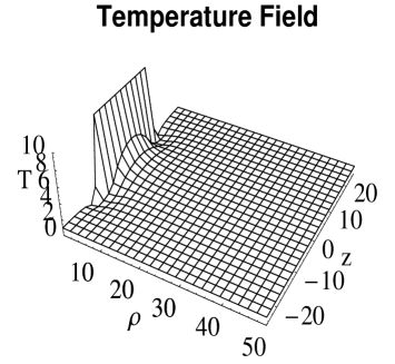
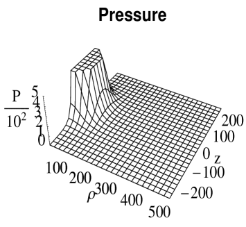
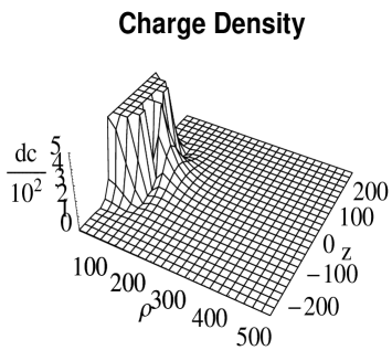
Figure 1: Profiles of the temperature, the mechanical pressure, the charge density and the energy density of the system. The values of the parameters are $T_{\infty}=1$, $m=1$, $\alpha=0.54$ and $\Phi_{0}=0.5$.

A thermodynamic analysis of the system can be made performing a decomposition of the energy-momentum tensor $T_{\alpha\beta}=\overset{(EM)}{T_{\alpha\beta}}+\overset{(F)}{T_{\alpha\beta}}$ in its proper components as made by Eckart Eck . Note that for static system Eckart’s thermodynamics does not present causality problems. Following Eckart, we can write the energy-momentum tensor in its proper components as

$$T^{\alpha\beta}=\xi v^{\alpha}v^{\beta}+Q^{\alpha}v^{\beta}+Q^{\beta}v^{\alpha}+\lambda^{\alpha\beta},$$ (36)

with $\xi$, $Q^{\alpha}$, $\lambda^{\alpha\beta}$ are given by

$$\xi=v_{\alpha}v_{\beta}T^{\alpha\beta},$$ (37)

$$Q^{\alpha}=-h^{\alpha}_{\beta}T^{\beta\gamma}v_{\gamma},$$ (38)

$$\lambda^{\alpha\beta}=h^{\alpha}_{\gamma}h^{\beta}_{\delta}T^{\gamma\delta}.$$ (39)

where $\xi$ is the energy density of the system, $Q^{\alpha}$ is the energy flux of the system and $\lambda^{\alpha\beta}$ is the stress tensor of the system. Calculating explicitly the components of the energy flux of the system, with the help of Eqs. (18) and (20), we found that $Q^{1}=Q^{2}=Q^{3}=0$ which means that the system is in an equilibrium configuration. In this case the temperature of the system obeys the relation Eck ; is2 ; his ,

$$h^{\alpha\beta}[\nabla_{\beta}T+Tv^{\mu}\nabla_{\mu}v_{\beta}]=0.$$ (40)

For $\alpha=1,2,3$ we have that

$$\partial_{\rho}\ln\left[T\sqrt{f}\right]=0,$$ (41)

$$\partial_{z}\ln\left[T\sqrt{f}\right]=0,$$ (42)

$$\partial_{\varphi}T=0.$$ (43)

Using the above equations we state that the temperature of the system is equal to

$$T(\rho,z)=\frac{T_{\infty}}{\sqrt{f}},$$ (44)

where $T_{\infty}$ is the temperature at infinity.

The mechanical pressure of the system ($P$) is given in Eckart’s thermodynamics by the expression

$$P = \frac{1}{3}g_{\alpha\beta}\lambda^{\alpha\beta}=\frac{1}{3}g_{\alpha\beta}h^{\alpha}_{\gamma}h^{\beta}_{\delta}T^{\gamma\delta}$$ (45)

$$= \frac{(1-\Phi_{0}^{2})f^{N}}{48\pi\rho e^{2\Lambda}}\overrightarrow{\nabla}\cdot\left(\frac{\rho}{f^{N}}\overrightarrow{\nabla}f\right),$$

where $N=(2-3\Phi_{0}^{2})/(2-2\Phi_{0}^{2})$. The energy density of the system (37) can be written as

$$\xi=\frac{\left(1+\Phi_{0}^{2}\right)f^{M}}{16\pi\rho e^{2\Lambda}}\overrightarrow{\nabla}\cdot\left(\frac{\rho}{f^{M}}\overrightarrow{\nabla}f\right),$$ (46)

where $M=(2+3\Phi_{0}^{2})/(2+2\Phi_{0}^{2})$.

In Fig. 1 we present a graph of the temperature, the mechanical pressure, the charge density and the energy density of the system. Note that all variables decay rapidly to their asymptotic values, which suggest that we can treat our system as a compact stellar object. While varying the values of the parameters $\Phi_{0}$, $\alpha$ and $m$ we found that we can obtain models which are less or more compact. For higher values of $\Phi_{0}$ we obtain the more compact objects.

V Conclusions

In this work we found an analytical axially symmetric static solution of Einstein’s equations with a energy-momentum tensor which couples an electromagnetic field and a fluid field. Far from the source, our metric is consistent with the Schwarzschild solution. Moreover, if we let $\Phi_{0}=0$ we recover the Gutsunaev-Manko solution. The thermodynamic variables studied in our model suggest that we can treat our model as a compact stellar object, and these variables also may allow a direct comparison with observations.

The solution to the Einstein equations presented in this work is a static metric. This looks like to be in contradiction to previous results that state that in the spacetime associated to a static magnetic dipole in the presence of electric charges appears a frame-dragging effect bon ; man:rod , i.e. we have a stationary metric. In our case, the static configuration is possible because the heat flux and the electromagnetic energy flux (20) compensate each other in such a way that the total energy flux is equal to zero. Static metrics associated to the equilibrium configurations obtained from the superposition of counterrotating fluxes in the context of General Relativity are not new, e.g, in the Morgan & Morgan disks mor:mor we have the same number of particles rotating in opposite directions (counterrotating hypothesis).

We conclude by mentioning that our solution that represents a charged fluid around a massive magnetic dipole may be useful to model a magnetar within a fluid.

VI Acknowledgment

J.D.P. thanks CNPQ for financial support and C. Dobrigkeit for valuable suggestions; P.S.L. thank FAPESP and CNPq for financial support.

APPENDIX A: FUNCTIONAL FORM OF $\Phi(f)$

To find the functional form of $\Phi$ first we write the function $f$ as a power series of $\Phi$

$$f=\sum_{n=0}^{\infty}a_{n}\Phi^{n},$$ (47)

where $a_{n}$ are real coefficients. Replacing (47) in (16), we obtain

$$\sum_{n=0}^{\infty}a_{n}\overrightarrow{\nabla}\cdot\left[\frac{\Phi^{n}}{\rho}\overrightarrow{\nabla}W\right]=a_{0}\overrightarrow{\nabla}\cdot\left[\frac{1}{\rho}\overrightarrow{\nabla}W\right]$$

$$+a_{1}\overrightarrow{\nabla}\cdot\left[\frac{\Phi}{\rho}\overrightarrow{\nabla}W\right]+\dots=0.$$ (48)

To simplify the notation we define the quantities $B_{n}$ as

$$B_{n}=\overrightarrow{\nabla}\cdot\left[\frac{\Phi^{n}}{\rho}\overrightarrow{\nabla}W\right],$$ (49)

with $n=0,1,2,3,\dots,\infty$, which satisfy the recurrence relation

$$B_{n}=2\Phi B_{n-1}-\Phi^{2}B_{n-2}.$$ (50)

With the help of Eq. (50) we can cast Eq. (48) into the form

$$\sum_{n=0}^{\infty}a_{n}B_{n}=B_{1}\sum_{n=1}^{\infty}(a_{n}-2a_{n+2})n\Phi^{n}$$

$$+B_{2}\sum_{n=2}^{\infty}(n-2)a_{n}\Phi^{n-2}=0.$$ (51)

To obtain one condition from Eq. (51) to help us to find the functional form $\Phi(f)$, we demand that $a_{n}=2a_{n+2}$ for all $n\geq 1$. This allows us to write the above series only in terms of $B_{2}$, say

$$\sum_{n=0}^{\infty}a_{n}B_{n}=\frac{1}{2}B_{2}\Phi^{2}\left[a_{1}\sum_{n=0}^{\infty}\frac{2n+1}{2^{n}}\Phi^{2n}\right.$$

$$\left.+a_{2}\sum_{n=0}^{\infty}\frac{n+1}{2^{n}}\Phi^{2n+1}\right]=0.$$ (52)

The above equation is satisfied if we set $B_{2}=0$, so

$$B_{2}=\overrightarrow{\nabla}\cdot\left[\frac{\Phi^{2}}{\rho}\overrightarrow{\nabla}W\right]=0.$$ (53)

Finally, by direct comparison between Eq. (53) and Eq. (16) we obtain that the functional form of $\Phi$ is $\Phi=\Phi_{0}\sqrt{f}$, where $\Phi_{0}$ is a constant. Note that by D’Alembert criterion the series of Eq. (47) converges when $|\Phi|<\sqrt{2}$.

APPENDIX B: SOLUTION OF EQS. (8) AND (26)

Using the prolate ellipsoidal coordinates defined as

$$\rho=k\sqrt{x^{2}-1}\sqrt{1-y^{2}},\;\;\;z=kxy,$$ (54)

where $k$ is a real parameter, we can write Eqs. (16) and (26) in the form

$$\left(\frac{f}{1-y^{2}}W_{,x}\right)_{,x}+\left(\frac{f}{x^{2}-1}W_{,y}\right)_{,y}=0,$$ (55)

$$\left(\frac{x^{2}-1}{f}f_{,x}-\frac{2\left(1-\Phi^{2}_{0}\right)}{k^{2}}\frac{Wf}{1-y^{2}}W_{,x}\right)_{,x}$$

$$+\left(\frac{1-y^{2}}{f}f_{,y}-\frac{2\left(1-\Phi^{2}_{0}\right)}{k^{2}}\frac{Wf}{x^{2}-1}W_{,y}\right)_{,y}=0.$$ (56)

Now, we define the auxiliary functions $H$ and $G$, so that $H=\frac{\sqrt{1-\Phi_{0}^{2}}}{k(1-y^{2})}W$ and $G=\frac{x+1}{x-1}f$. With these definitions, Eq. (55) is trivially satisfied by a function $I(x,y)$ if

$$I_{,y}=\frac{x-1}{x+1}GH_{,x},$$ (57)

$$I_{,x}=-\frac{G}{(x+1)^{2}}[(1-y^{2})H]_{,y}.$$ (58)

So, Eq. (56) can be written in terms of $G$, $H$ and $I$, say

$$\left(I_{,yy}-I_{,xx}\right)H=$$ (59)

$$\frac{x^{2}-y^{2}}{1-y^{2}}\left(\left[\frac{G_{,x}}{2G}\right]_{,y}+\frac{\left(x+1\right)I_{,x}I_{,y}}{G\left(x-1\right)}\right).$$

The next step is to assume that $G$, $H$ and $I$ are functions of the form

$$I=\frac{N}{D},\mbox{\hskip 14.22636pt}H=\frac{S}{M}\mbox{\hskip 14.22636ptand \hskip 14.22636pt}G=\frac{M^{2}}{D^{2}},$$ (60)

where $N,D,S$ and $M$ are polynomials in $x$ and $y$ of the form,

$$N(x,y)=\sum_{j=0}^{j_{max}}\sum_{m=0}^{j_{max}-j}\eta_{jm}x^{j}y^{m}$$ (61)

$$S(x,y)=\sum_{j=0}^{j_{max}}\sum_{m=0}^{j_{max}-j}\sigma_{jm}x^{j}y^{m}$$ (62)

$$D(x,y)=\sum_{j=0}^{j_{max}}\sum_{m=0}^{j_{max}-j}\delta_{jm}x^{j}y^{m}$$ (63)

$$M(x,y)=\sum_{j=0}^{j_{max}}\sum_{m=0}^{j_{max}-j}\mu_{jm}x^{j}y^{m}$$ (64)

with $\eta_{jm}$, $\sigma_{jm}$, $\delta_{jm}$, $\mu_{jm}$ being unknown coefficients to be determined. Substituting the relations (60) into Eqs. (57) and (58) we obtain the set of equations

$$(x+1)(DN_{,y}-ND_{,y})-(x-1)(MS_{,x}-SM_{,x})=0,$$

$$(x+1)^{2}(DN_{,x}-ND_{,x})+M^{2}\left[(1-y^{2})\frac{S}{M}\right]_{,y}=0.$$

(65)

The system of Eqs (65), together with Eq. (59) can be solved in a tedious direct comparison of the coefficients of the polynomials involved. The solution depends on the number of coefficients for each polynomial, i.e. the value of $j_{max}$. Furthermore, we impose that the solution obtained be symmetric on the plane $z=0$ and also that has the Schwarzschild solution as a particular case. The first physical solution is obtained when $j_{max}=4$. In this case the coefficients can be written in terms of only one parameter, $\alpha$. The solution is

$$N=8\alpha^{3}xy\left(x-1\right),$$

$$D=\left[x^{2}-y^{2}+\alpha^{2}(x-1)^{2}\right]^{2}-4\alpha^{2}y^{2}(x^{2}-1),$$

$$M=\left[x^{2}-y^{2}+\alpha^{2}(x^{2}-1)\right]^{2}+4\alpha^{2}x^{2}(1-y^{2}),$$

$$S=4\alpha^{3}\left[2x^{3}+\frac{\left(1-3\alpha^{2}\right)}{\left(\alpha^{2}+1\right)}x^{2}+\frac{y^{2}+\alpha^{2}}{\left(\alpha^{2}+1\right)}\right].$$ (66)

Using the solution (66), the functions $f$, $\Phi$ and $W$ are known. The function $\Lambda$ is calculated integrating Eqs. (13) and (14).

References

- (1) A. Akmal, V.R. Pandharipande and D.G. Ravenhall, Phys. Rev. C 58, 1804 (1998).
- (2) K. Fukushima and H.J. Warringa, Phys. Rev. Lett. 100, 032007 (2008).
- (3) H. Sotani, A. Colaiuda and K.D. Kokkotas, MNRAS, Online Early doi:10.1111/j.1365-2966.2008.12977.x
- (4) D.N. Aguilera, J.A. Pons and J.A. Miralles, ApJ 673, L167 (2008).
- (5) K.E. Kunze, Phys. Rev. D 77, 023530 (2008).
- (6) A.P. Lobanov, A&A 330, 79 (1998).
- (7) F.A. Aharonian, MNRAS 332, 215 (2002).
- (8) A.F. Zakharov et al, MNRAS 342, 1325 (2003).
- (9) J.S. Greaves et al, Nature 404, 732 (2000).
- (10) Y.T. Liu, S.L. Shapiro and B.C. Stephens, Phys. Rev. D 76, 084017 (2007).
- (11) S. Akiyama et al, ApJ 584, 954 (2003).
- (12) W.H.T. Vlemmings, P.J. Diamond and H. Imai, Nature 440, 58 (2006).
- (13) D.L. Meier, S. Koide and Y.Uchida, Science 291, 84 (2001).
- (14) G.V. Ustyugova et al, ApJ 516, 221 (1999).
- (15) R. Krasnopolsky, Z.Y. Li and R.D. Blandford, ApJ 595, 631 (2003).
- (16) P. Hennebelle and S. Fromang, A&A 477, 9 (2008).
- (17) Z. Medin and D. Lai, MNRAS 382, 1833 (2007).
- (18) X.D. Li and E.P.J. van den Heuvel, ApJ 513, L45 (1999).
- (19) G.G. Pavlov and V.G. Bezchastnov, ApJ 635, L61 (2005).
- (20) A.I. Ibrahim, J.H. Swank and W. Parke, ApJ 584, L17 (2003).
- (21) K. Schwarzschild, Sitzungsberichte der Königlich Preussischen Akademie der Wissenschaften 1, 189 (1916).
- (22) K. Schwarzschild, Sitzungsberichte der Königlich Preussischen Akademie der Wissenschaften 1, 424 (1916).
- (23) R.P. Kerr, Phys. Rev. Lett. 11, 237 (1963).
- (24) E.T. Newman et al, J. Math. Phys. 6, 918 (1965).
- (25) H. Reissner, Ann. Phys. Berlin 50, 106 (1916).
- (26) G. Nordström, Verhandl. Koninkl. Ned. Akad. Wetenschap. 20, 1231 (1918).
- (27) R.C. Tolman, Phys. Rev. 55, 364 (1939).
- (28) J.R. Oppenheimer and G.M. Volkoff, Phys. Rev. 55, 374 (1939).
- (29) B. Brügmann, W. Tichy and N. Jansen, Phys. Rev. Lett. 92, 211101 (2004).
- (30) M. Alcubierre et al, Classical Quantum Gravity 21, 589 (2004).
- (31) J.A. Font, Living Rev. Relativity 4, 1 (2003).
- (32) Ts.I. Gutsunaev , V.S. Manko, Phys. Lett. A 123, 215 (1987).
- (33) C. Eckart, Phys. Rev. 58, 919 (1940).
- (34) W. Israel and J.M. Stewart, Ann. Physics 118, 341 (1979).
- (35) W.A. Hiscock and L. Lindblom, Ann. Physics 151, 466 (1983).
- (36) W. Bonnor, Phys. Lett. A 158, 23 (1991).
- (37) V.S. Manko, E.D. Rodchenko, B.I. Sadovnikov and J. Sod-Hoffs, Class. Quantum Grav. 23, 5389 (2006).
- (38) T. Morgan and L. Morgan, Phys. Rev. 183, 1097 (1969).