Phase Transition with Non-Thermodynamic States in Reversible Polymerization

Abstract

We investigate a reversible polymerization process in which individual polymers aggregate and fragment at a rate proportional to their molecular weight. We find a nonequilibrium phase transition despite the fact that the dynamics are perfectly reversible. When the strength of the fragmentation process exceeds a critical threshold, the system reaches a thermodynamic steady state where the total number of polymers is proportional to the system size. The polymer length distribution has a sharp exponential tail in this case. When the strength of the fragmentation process falls below the critical threshold, the steady state becomes non-thermodynamic as the total number of polymers grows sub-linearly with the system size. Moreover, the length distribution has an algebraic tail and the characteristic exponent varies continuously with the fragmentation rate.

I Introduction

Equilibrium systems relax to a steady state described by the Gibbs distribution. In contrast, nonequilibrium systems are specified by the dynamics rather then by a Hamiltonian, and there is no general framework for describing nonequilibrium steady states. Furthermore, unlike equilibrium phase transitions that are characterized by robust universality classes jes , nonequilibrium phase transitions are highly sensitive to details of the underlying dynamics hh .

In this paper, we investigate polymerization dynamics, and we report that competition between aggregation and fragmentation results in a remarkable non-equilibrium phase transition. Despite the fact that the dynamics are perfectly reversible, there is a nonequilibrium phase transition from a thermodynamic state where the number of polymers is proportional to the system size into a non-thermodynamic state where the number of polymers is not proportional to the system size.

Reversible polymerization is ubiquitous in polymer and atmospheric chemistry pjf ; rld ; sp , and has analogies in networks ab and computer science bb ; dja ; jlr . Reversible polymerization includes two competing processes: (i) The aggregation process $[i]+[j]\to[i+j]$, merger of two polymer chains of lengths $i$ and $j$ into a larger polymer, occurs with the aggregation rate $K_{ij}$; (ii) The fragmentation process $[i+j]\to[i]+[j]$, breakage of a polymer into two smaller polymers, proceeds with rate $F_{ij}$. This process is reversible because the aggregation process and the fragmentation process perfectly mirror each other.

Reversible polymerization is described by the master equations note

$$\frac{dc_{k}}{dt} = \frac{1}{2}\sum_{i+j=k}K_{ij}\,c_{i}\,c_{j}-c_{k}\!\sum_{j\geq 1}K_{kj}\,c_{j}$$ (1)

$$+ \sum_{j\geq 1}F_{kj}\,c_{j+k}-\frac{1}{2}\,c_{k}\!\sum_{i+j=k}F_{ij}$$

where $c_{k}(t)$ is the density of polymer chains composed of $k$ monomers at time $t$. The first two terms describe changes due to aggregation and the next two terms account for changes due to fragmentation. The aggregation and fragmentation rates are (non-negative) symmetric matrices, $K_{ij}=K_{ji}$ and $F_{ij}=F_{ji}$.

In the simplest case, the steady state distribution is found by equating the aggregation flux with the fragmentation flux,

$$K_{ij}\,c_{i}\,c_{j}=F_{ij}\,c_{i+j}.$$ (2)

This detailed balance condition specifies an equilibrium state where the fluxes between any two microscopic states of the system balance. Such an equilibrium steady state exists for example when both the aggregation and the fragmentation rates are constant bt . Another equilibrium state was found in a model of strings at very high-temperatures with the rates $K_{ij}=ij$ and $F_{ij}=i+j$ lt .

The detailed balance equation (2) admits a solution only when the aggregation and fragmentation rates satisfy special relations, as shown in Appendix A. In general, the steady state distribution is specified by the full master equations (1) and moreover, the detailed balance relations (2) may very well be violated. For example, in a “chipping” process where only end-monomers can detach from the polymer, the matrix $F_{ij}$ is sparse: $F_{ij}=0$ when both $i,j\geq 2$. For constant aggregation rates, the chipping process exhibits a nonequilibrium phase transition. When the fragmentation rate falls below a certain threshold, a giant macroscopic polymer emerges vzl ; kr ; mkb ; rm .

We consider the aggregation and fragmentation rates

$$K_{ij}=ij,\qquad F_{ij}=\lambda.$$ (3)

These rates, while intermediate between the linear chain model bt and the string model lt , violate detailed balance (see Appendix A). The product aggregation rate accounts for the natural situation in which any two monomers may form a chemical bond, thereby leading to merger of their respective polymers. This polymerization process has been widely studied in polymer chemistry pjf1 ; whs ; jdb ; jls ; ve and in the context of percolation sa ; fl ; zhe ; aal . The constant fragmentation rate reflects situations where all chemical bonds in the linear polymer are equally likely to break, thereby leading to breakage into two smaller polymers. This de-polymerization process has also been studied extensively zm . Like the aggregation rate, the total fragmentation rate is linear in the molecular weight, $\sum_{i+j=k}F_{ij}=\lambda(k-1)$.

Starting with $N$ monomers, we study the nonequilibrium steady states that emerge in the reversible polymerization process (3). We find that the system generally reaches a steady state, and that a nonequilibrium phase transition occurs at the critical fragmentation rate $\lambda_{c}=1$. The average total number of polymers, $N_{\rm tot}$, grows algebraically with the system size $N$,

$$N_{\rm tot}\sim N^{\gamma}\qquad{\rm with}\qquad\gamma=\frac{2\lambda}{2+\lambda},$$ (4)

when fragmentation is weak, $\lambda<\lambda_{c}$. The total number of polymers grows sub-linearly with the system size because $\gamma<1$. Moreover, large polymers are likely as the polymer size distribution has a broad algebraic tail. The system develops this non-thermodynamic state through a gelation transition. We probe this gelation using moments of the size distribution.

In contrast, the system reaches an ordinary steady state when the fragmentation process is strong. The average total number of polymers is proportional to the system size, $N_{\rm tot}=(1-\lambda^{-1})N$, when $\lambda>\lambda_{c}$. Large polymers become rare since the polymer size distribution has a sharp exponential tail.

Interestingly, even though the polymerization process is reversible because the underlying aggregation ($[i]+[j]\to[i+j]$) and fragmentation ($[i+j]\to[i]+[j]$) processes perfectly mirror each other and none of the transition rates (3) vanish, the breakdown of detailed balance leads to a remarkable phase transition involving a non-thermodynamic phase where the number of polymers is not proportional to the system size and a thermodynamic phase where the number of polymers is proportional to the system size.

The rest of this paper is organized as follows. The thermodynamic steady states that occur under strong fragmentation are examined in the next section, while the non-thermodynamic steady states that emerge when fragmentation is weak are analyzed in section III. The gelation transition is probed using the moments of the size distribution in section IV. Monte Carlo simulation results validating the theoretical predictions for the non-thermodynamic phase are detailed in section V. We discuss the results and several open-ended questions in section VI. Appendices A–C contain several technical derivations.

II Thermodynamic Phase

Our focus is the steady state behavior and in particular, the stationary polymer size density $c_{k}$ that satisfies

$$\frac{1}{2}\!\sum_{i+j=k}ij\,c_{i}c_{j}-k\,c_{k}=-\lambda\sum_{j>k}^{\infty}c_{j}+\frac{\lambda}{2}\,(k-1)c_{k}.$$ (5)

This steady state equation is obtained by substituting the aggregation and fragmentation rates (3) into the stationary master equation (1). At the steady state, changes due to aggregation, represented on the left hand side, balance changes due to fragmentation, represented on the right hand side. Since both aggregation and fragmentation do not alter the total mass, the overall mass density $\sum_{k}kc_{k}$ is a conserved quantity, as follows from the rate equation (1). We conveniently set the normalization $\sum_{k}kc_{k}=1$ without loss of generality.

The total polymer density $M_{0}=\sum_{k}c_{k}$ is the most elementary probe for the state of the system. At the steady state, this quantity satisfies

$$\frac{1}{2}=\frac{\lambda}{2}\left(1-M_{0}\right),$$ (6)

an equation obtained by summing (5) and by using the identity $\sum_{k}\sum_{j\geq k}c_{j}=\sum_{j}c_{j}\sum_{k<j}1=\sum_{j}(j-1)c_{j}$ and the normalization condition $\sum_{k}kc_{k}=1$. The total density is non-zero

$$M_{0}=1-\lambda^{-1},$$ (7)

when the fragmentation rate is sufficiently strong, $\lambda>1$. We focus on this strong fragmentation regime in the rest of this section.

Let us assume that the system is large but finite with a total mass equal $N$, a state that can be achieved by starting with $N$ monomers, for example. The expected total number of polymers, $N_{\rm tot}=N\sum_{k}c_{k}=NM_{0}$ is proportional to the system size $N$, and therefore, the system is in a thermodynamic state.

The polymer size density can be calculated by utilizing the recurrent nature rec_nat of Equation (5). For instance, the monomer and the dimer densities are

$$c_{1} =\frac{\lambda-1}{\lambda+1},$$ (8a)

$$c_{2} =\frac{(\lambda-1)(3\lambda+1)}{(\lambda+1)^{2}(3\lambda+4)}.$$ (8b)

In general, the polymer size density is finite in the thermodynamic phase, $\lambda>1$. Very large polymers are rare since the size distribution decays exponentially

$$c_{k}\simeq Ak^{-5/2}\,e^{-ak},$$ (9)

when $k\to\infty$. This result is derived in Appendix B.

When fragmentation is extremely strong, the system consists primarily of monomers: $c_{1}=1+O(\lambda^{-1})$ and $c_{2}=\lambda^{-1}+O(\lambda^{-2})$ when $\lambda\to\infty$. The leading asymptotic behavior can be obtained exactly in this strong fragmentation limit,

$$c_{k}\simeq\frac{k^{k-2}}{k!}\left(\frac{2}{\lambda}\right)^{k-1},$$ (10)

for all $k$. This expression, obtained in Appendix C, is compatible with the generic exponential tail (9).

The near-critical behavior

The total density, the monomer density, and the dimer density all vanish near the transition point, $M_{0}\simeq(\lambda-1)$, $c_{1}\simeq\frac{1}{2}(\lambda-1)$, and $c_{2}\simeq\frac{1}{7}(\lambda-1)$ as $\lambda\to 1$. This behavior suggests the perturbative approach,

$$c_{k}=\epsilon\,b_{k}$$ (11)

with the small parameter $\epsilon=\lambda-1$. The first two coefficients are $b_{1}=\frac{1}{2}$ and $b_{2}=\frac{1}{7}$. We substitute this form into the stationary equation (5) and observe that the nonlinear aggregation term $\propto\epsilon^{2}$ is negligible. Consequently, to leading order, the polymer size density obeys the linear recursion equations

$$k\,b_{k} =\sum_{j=k+1}^{\infty}b_{j}-\frac{1}{2}\,(k-1)b_{k},$$ (12a)

$$(k+1)b_{k+1} =\sum_{j=k+2}^{\infty}b_{j}-\frac{1}{2}\,k\,b_{k+1}.$$ (12b)

The second equation is obtained from the first by an index shift. We subtract the two equations and obtain a recursion relation for the coefficients $b_{k}$,

$$\frac{b_{k+1}}{b_{k}}=\frac{k-\frac{1}{3}}{k+\frac{4}{3}}.$$ (13)

The coefficients can be conveniently expressed as a ratio of Gamma functions, $b_{k}\propto\Gamma(k-1/3)/\Gamma(k+4/3)$, by using the identity $\Gamma(x+1)/\Gamma(x)=x$. The polymer size density is therefore

$$b_{k}=\frac{1}{2}\frac{\Gamma(\frac{7}{3})}{\Gamma(\frac{2}{3})}\frac{\Gamma(k-\frac{1}{3})}{\Gamma(k+\frac{4}{3})},$$ (14)

where the proportionality constant is set by $b_{1}=\frac{1}{2}$.

Near criticality, the size density is algebraic,

$$c_{k}\sim\epsilon\,k^{-5/3},$$ (15)

over a substantial range, $k\ll k_{*}$. This result follows from (14) and $\lim_{x\to\infty}x^{a}\Gamma(x)/\Gamma(x+a)=1$. Therefore, the likelihood of finding large polymers becomes substantial as the phase transition point is approached. The cutoff scale $k_{*}$, set by mass conservation, $\sum_{k=1}^{k_{*}}kc_{k}=1$, is divergent

$$k_{*}\sim\epsilon^{-3}\,.$$ (16)

The size distribution is sharply suppressed according to (9) beyond this scale. Using the relation $A\sim a^{-1/2}$, derived in appendix B, and $a\sim k_{*}^{-1}$ we deduce that

$$c_{k}\sim\epsilon^{-3/2}k^{-5/2}e^{-{\rm const}\times{\epsilon^{3}}\,k}$$ (17)

for $k\gg k_{*}$. Indeed, this large size behavior matches the small size behavior (15) at the crossover scale (16). We conclude that the convolution term, that accounts for the creation of very large polymers from smaller polymers, is relevant only at very large scales, $k\gg k_{*}$. Otherwise, this term does not affect the density of small polymers.

For completeness, we mention that the leading asymptotic behavior of the moments, $M_{n}=\sum_{k}k^{n}c_{k}$, readily follows from the density (15) and the cutoff (16),

$$M_{n}\sim\begin{cases}\epsilon^{-3(n-1)}&n>2/3\\ 1&n<2/3.\end{cases}$$ (18)

Sufficiently large order moments diverge in the vicinity of the transition point, a consequence of the algebraic tail (15). The low order moments are finite, however.

III Non-thermodynamic Phase

As the critical point is approached, the nonlinear convolution term in (5) becomes irrelevant over the divergent scale (16). By continuity, we deduce that the convolution term is negligible when $\lambda<1$. Consequently, the stationary distribution obeys the linear equation

$$k\,c_{k}=\lambda\left(\sum_{k=1}^{\infty}c_{k}-\sum_{j=1}^{k}c_{j}\right)-\frac{\lambda}{2}\,(k-1)c_{k}$$ (19)

when $\lambda<1$. We introduce the normalized size density, $\rho_{k}=c_{k}/\sum_{k}c_{k}$, with $\sum_{k\geq 1}\rho_{k}=1$. With this transformation, the stationary equation (19) becomes

$$k\,\rho_{k}=\lambda\left(1-\sum_{j=1}^{k}\rho_{j}\right)-\frac{\lambda}{2}\,(k-1)\rho_{k}.$$ (20)

The monomer and dimer densities follows immediately,

$$\rho_{1} =\frac{\lambda}{1+\lambda},$$ (21a)

$$\rho_{2} =\frac{2\lambda}{(1+\lambda)(4+3\lambda)}.$$ (21b)

The normalized densities undergo a phase transition at $\lambda_{c}=1$, as shown in figure 1. The fraction of monomers is not affected by the convolution term and (21a) holds for all $\lambda$. However, the dimer density (21b) differs from the expression $\rho_{2}=\frac{\lambda(1+3\lambda)}{(1+\lambda)^{2}(4+3\lambda)}$ for $\lambda<1$ implied by (8b) and (7). Similarly, the normalized size densities $\rho_{k}$ exhibit a phase transition for all $k>1$.

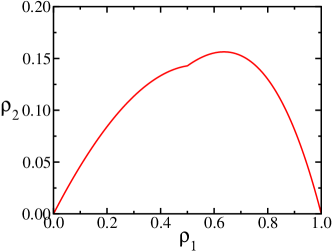
Figure 1: The normalized dimer density $\rho_{2}$ versus the normalized monomer density $\rho_{1}$. The phase transition at $\lambda_{c}=1$ is reflected by the discontinuity in the first derivative at $\rho_{1}=1/2$.

Generally, we recast Eq. (20) into the following recursion for the normalized densities

$$\frac{\rho_{k+1}}{\rho_{k}}=\frac{k-\frac{\lambda}{2+\lambda}}{k+\frac{2(1+\lambda)}{2+\lambda}}.$$ (22)

This recursion is obtained by repeating the steps leading to (13). Again, we express the normalized densities as a ratio of Gamma functions, $\rho_{k}\propto\Gamma(k-\frac{\lambda}{2+\lambda})/\Gamma(k+\frac{2(1+\lambda)}{2+\lambda})$. The monomer density (21a) sets the proportionality constant and hence,

$$\rho_{k}=\frac{\lambda}{1+\lambda}\frac{\Gamma\left(1+\frac{2(1+\lambda)}{2+\lambda}\right)}{\Gamma\left(1-\frac{\lambda}{2+\lambda}\right)}\frac{\Gamma\left(k-\frac{\lambda}{2+\lambda}\right)}{\Gamma\left(k+\frac{2(1+\lambda)}{2+\lambda}\right)}.$$ (23)

The size density has an algebraic tail,

$$\rho_{k}\sim k^{-\beta}\qquad{\rm with}\qquad\beta=\frac{2+3\lambda}{2+\lambda},$$ (24)

as $k\to\infty$, thereby implying that large polymers are likely. The decay exponent $1<\beta<5/3$ is not universal.

The size density obeys $c_{k}\propto\rho_{k}$, and the $N$-dependent proportionality constant is obtained from the mass conservation condition $\sum_{k=1}^{N}kc_{k}=1$ where the upper limit of integration is set by the system size. This sum is dominated by the density of large polymers. By performing the summation, we find that the polymer size density depends on the system size

$$c_{k}\sim N^{\beta-2}k^{-\beta}.$$ (25)

The total number of clusters $N_{\rm tot}\sim N\sum_{k}c_{k}$ grows sub-linearly with the system size $N_{\rm tot}\sim N^{\gamma}$ with $\gamma=\beta-1$ as announced in (4). Therefore, the total polymer density, $M_{0}\sim N^{\beta-2}$, depends on the system size in contrast with the behavior when $\lambda>1$. In deriving the steady state equation (19), we assumed that the convolution term is negligible. This assumption is consistent with the fact that the amplitude $N^{\beta-2}$ in (25) vanishes as the system size diverges.

Moreover, the expected total number of polymer of size $k$, $C_{k}=Nc_{k}$, is as follows, $C_{k}\sim N^{\gamma}k^{-\beta}$ with $\gamma=\frac{2\lambda}{2+\lambda}$. This steady state is not thermodynamic! The number of polymers is much smaller then the system size, yet the number of polymers still diverges with the total mass: $C_{k}$ grows sub-linearly with the system size because $\gamma<1$.

For irreversible polymerization, $\lambda=0$, all mass eventually ends up in a single giant polymer, as reflected by the characteristic exponent $\gamma=0$. The total number of polymers still grows sub-linearly, $N_{\rm tot}\sim N^{2/3}$, when the critical point is approached, $\lambda\to 1$.

In the thermodynamic phase, all polymers are finite in size. Indeed, the exponential tail behavior (9) implies that the largest polymers are finite in scale. Near criticality, the scale of the largest polymers diverges according to (16). In the non-thermodynamic phase, there are polymers of all possible scales because the power-law behavior (25) holds up to the system size $\propto N$. Remarkably, there are polymers that contain a finite fraction of all the mass in the system because according to (25), the total number of macroscopic clusters, $N\sum_{k\geq{\rm const.}\times N}c_{k}$ is of the order one.

The power-law distribution (24) accounts for a competition between two fluxes. There is a flux of mass from small scales to large scales that is generated by the aggregation process and a flux from large scale to small scales caused by fragmentation. The power-law behavior holds for all scales, indicating that these two fluxes balance at all intermediate scales. Similar competitions between the fluxes occur in fluid turbulence fluid , passive scalar advection passive , wave turbulence zlf , granular gases bm , and driven aggregation systems ht ; kmr ; crz . However, reversible polymerization differs from these driven system in that there is no external injection of mass to maintain the steady-state.

IV The Gelation Transition

We now study the approach toward the steady state specified by the full master equation

$$\frac{dc_{k}}{dt}=\frac{1}{2}\!\!\sum_{i+j=k}\!\!ij\,c_{i}c_{j}-k\,c_{k}+\lambda\!\sum_{j>k}^{\infty}\!c_{j}-\frac{\lambda}{2}\,(k-1)c_{k}.$$ (26)

Initially, there are only monomers, $c_{k}(t=0)=\delta_{k,1}$.

First, we consider the total polymer density $M_{0}$ that obeys the linear rate equation

$$\frac{dM_{0}}{dt}=-\frac{1}{2}+\frac{\lambda}{2}\,(1-M_{0}).$$ (27)

Subject to the initial condition $M_{0}(0)=1$, the total density is

$$M_{0}=1-\lambda^{-1}+\lambda^{-1}\,e^{-\lambda t/2}.$$ (28)

Hence, the steady state (7) is approached exponentially fast in the thermodynamic phase. Moreover, the monomer and the dimer densities also relax exponentially fast as in (28) and in general, the polymer size density quickly approaches the steady state when $\lambda>1$.

We focus on the kinetics in the more interesting non-thermodynamic phase where the total polymer density (28) vanishes at time $t_{0}=\frac{2}{\lambda}\ln\frac{1}{1-\lambda}$. This behavior is consistent with the vanishing total density, $M_{0}\sim N^{\beta-2}$, implied by (25). Of course, the negative expression (28) is invalid beyond the time $t_{0}$.

The moments $M_{n}=\sum_{k}k^{n}c_{k}$ provide a direct probe of the kinetics. In the non-thermodynamic phase, the system nucleates large macroscopic gels and consequently, large moments diverge with the system size as follows from (25). This, together with the vanishing overall density $M_{0}$, indicates that the system undergoes a gelation transition at a finite time. At the gelation time $t_{g}$, a giant polymer or a gel emerges as is the case for irreversible polymerization ($\lambda=0$). From the master equation (26), the moments evolve according to

$$\frac{dM_{n}}{dt} = \frac{1}{2}\sum_{m=1}^{n-1}\binom{n}{m}M_{m+1}M_{n+1-m}-\frac{\lambda}{2}\,\frac{n-1}{n+1}\,M_{n+1}$$ (29)

$$+ \frac{\lambda}{n+1}\sum_{m=2}^{n}\binom{n+1}{m}B_{m}M_{n+1-m}$$

where $B_{m}$ are the Bernoulli numbers gkp . For example, the second moment obeys $dM_{n}/dt=M_{2}^{2}-\frac{\lambda}{6}(M_{3}-1)$. We assume that large order moments diverge algebraically at the gelation time, $M_{n}\sim(t_{g}-t)^{-(an+b)}$ for $n\geq 1$, and observe that the last term in the hierarchical equation (29) is negligible compared with the rest of the terms. We require that the time dependent term, the aggregation term, and the remaining fragmentation term are comparable and find that $a=-b=1$. Hence,

$$M_{n}\sim(t_{g}-t)^{-(n-1)}$$ (30)

for $n\geq 1$. Indeed, the moments diverge at a finite time. The exponent $n-1$ characterizing this divergence is compatible with the near critical behavior (18). The divergence (30) is different than the $M_{n}\sim(t_{g}-t)^{-(2n-3)}$ behavior in irreversible fragmentation fl , and therefore, fragmentation quantitatively alters the nature of the gelation transition.

We conclude that the solution to the master equation (26) exhibits a finite time singularity. Even though we can not obtain the gelation time $t_{g}$ exactly, relevant properties of the size density including the moments can still be obtained analytically. In particular, the form of the size density at the gelation time can be calculated by balancing the fluxes of mass due to aggregation and fragmentation, following the scaling analysis in ref. ve1 .

Consider $M^{(n)}$, the total mass density of polymers with size smaller then $n$,

$$M^{(n)}(t)=\sum_{k=1}^{n}kc_{k}(t).$$ (31)

According to the master equation (26), this quantity obeys

$$\frac{dM^{(n)}}{dt}\!=\!-\sum_{i=1}^{n}\!\sum_{j+i=n-1}^{\infty}\!\!i^{2}jc_{i}c_{j}+\frac{1}{2}\,\lambda n(n+1)\!\!\!\sum_{j=n+1}^{\infty}c_{j}.$$ (32)

We now take the $n\to\infty$ limit. The aggregation loss term accounts for loss of finite size polymers to the infinitely large gel while the fragmentation term accounts for the balancing flux from the gel into small masses. We require that the two fluxes balance at the gelation point. We assume that at the gelation point, the size density decays algebraically

$$c_{k}(t=t_{g})\sim k^{-\tau},$$ (33)

for $k\gg 1$, as is the case for irreversible polymerization zhe . By dimensional counting, the aggregation flux term scales as $n^{5-2\tau}$ while the fragmentation flux scales as $n^{3-\tau}$. The two fluxes balance when $5-2\tau=3-\tau$ and as a result $\tau=2$. Therefore, $c_{k}(t=t_{g})\sim k^{-2}$, a behavior that is consistent with the aforementioned divergence of the moments (30) when the power-law behavior (33) holds up to a cutoff scale that diverges near gelation, $k\ll(t_{g}-t)^{-1}$.

The normalization condition $\sum_{k}kc_{k}=1$ imposes the exponent restriction $\tau>2$ but the heuristic argument above yields precisely the marginal value $\tau=2$. We therefore anticipate that there is a logarithmic correction with the following form $c_{k}\sim k^{-2}(\ln k)^{-\mu}$. We substitute this form into (32) and then, the aggregation term is of the order $n\,[\ln n]^{1-2\mu}$ while the fragmentation term is of the order $n\,[\ln n]^{-\mu}$. Therefore, $\mu=1$, and nested

$$c_{k}\sim k^{-2}[\ln k]^{-1}$$ (34)

for $k\gg 1$. This decay is milder then the $c_{k}\sim k^{-5/2}$ behavior found for irreversible polymerization zhe , and therefore, there are many more large clusters in reversible polymerization.

The size of the largest gel at the gelation transition follows immediately from the extreme statistics criterion, $N\sum_{k=1}^{k_{g}}c_{k}=1$. Remarkably, this size is nearly macroscopic in the size of the system,

$$k_{g}\sim N[\ln N]^{-1}.$$ (35)

This gel size is much larger compared with the $k_{g}\sim N^{2/3}$ behavior in reversible polymerization. This increased scale enables the gel to withstand fragmentation. We also comment that the nearly macroscopic size scale (35) provides the appropriate cutoff in (31), $n\sim k_{g}$, and that at the gelation point, the upward mass aggregation flux and the downward mass fragmentation flux are nearly macroscopic, that is, they are proportional to the system size up to a logarithmic correction.

The critical case

For completeness, we discuss kinetics in the critical case $\lambda=1$ where the the cluster density (28) is purely exponential, $M_{0}=e^{-t/2}$. Similar decay characterizes the leading behavior of the size density. For example, the monomer density obeys $dc_{1}/dt=-c_{1}+(M_{0}-c_{1})$ and consequently,

$$c_{1}=\frac{2}{3}\,e^{-t/2}+\frac{1}{3}\,e^{-2t}.$$ (36)

Only the first term is relevant asymptotically, $c_{1}\simeq\frac{2}{3}\,e^{-t/2}$. In general, $c_{k}\simeq u_{k}\,e^{-t/2}$, and by substituting this expression into the time dependent master equation (26), we observe that the nonlinear term is negligible. Consequently, the coefficients $u_{k}$ satisfy the recursion equation

$$\left(k-\frac{1}{2}\right)u_{k}=\sum_{j=k+1}^{\infty}u_{j}-\frac{1}{2}(k-1)u_{k}.$$ (37)

From this recursion, the coefficients $u_{k}$ satisfy $u_{k+1}/u_{k}=(k-2/3)/(k+1)$. Therefore, the leading behavior of the size density is as follows

$$u_{k}=\frac{2}{3\Gamma(\frac{1}{3})}\frac{\Gamma(k-\frac{2}{3})}{\Gamma(k+1)}.$$ (38)

The tail of the size density matches the near critical behavior (15), $c_{k}\sim e^{-t/2}k^{-5/3}$.

V Numerical Simulations

We performed numerical simulations to validate the theoretical predictions. Below, we present results for the non-thermodynamic phase.

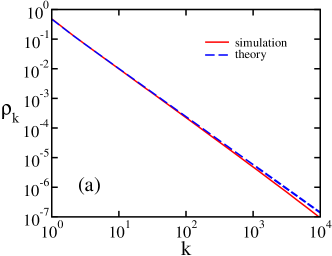
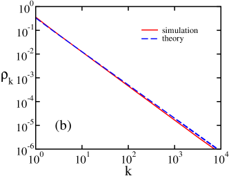
Figure 2: The size distribution $\rho_{k}$ versus $k$ for $\lambda=0.9$ (a) and $\lambda=0.5$ (b). The simulations results are for a system of size $N=10^{5}$.

The simulations were performed by starting with $N$ monomers and were carried by repeating the following Monte Carlo step. At each step, the total aggregation rate $R_{a}=\frac{1}{N}\sum_{i\neq j}s_{i}s_{j}$ and the total fragmentation rate $R_{f}=2\sum_{i}(s_{i}-1)$ are calculated where $s_{i}$ is the size of the $i$th polymer. Of course, both of these rates are proportional to the system size, $R_{a}\propto R_{f}\propto N$. An aggregation event is executed with probability $R_{a}/(R_{a}+R_{f})$, while a fragmentation event is executed with the complementary probability $R_{f}/(R_{a}+R_{f})$. In each aggregation event, one polymer is chosen with probability proportional to its size and is merged with another polymer, also chosen with probability proportional to its size. In a fragmentation event, a polymer, randomly chosen with probability proportional to the number of its bonds, is randomly split into two smaller polymers. Time is updated by the inverse of the total rate $t\to t+(R_{a}+R_{f})^{-1}$ after each Monte Carlo step. As a check, we successfully reproduced the total polymer density (7).

In the non-thermodynamic phase, the system undergoes a gelation transition and then relaxes to the steady state. We run the simulations until the system relaxed to the steady state and then obtained the size distribution from a long series of measurements to reduce statistical fluctuations. The simulations results are for systems of size $N=10^{5}$. We present results for the normalized densities $\rho_{k}$ predicted in (23). Overall, there is very good agreement between the theoretical predictions and the simulation results as shown in figure 2. The size distribution agrees with (23) and the tail of the distribution follows a power-law as in (24). The simulation results agree with the theoretical results slightly better near the phase transition point (Figures 2a and 2b). Since the total number of clusters grows sub-linearly with the system size, $N_{\rm tot}\sim N^{\gamma}$ with $\gamma<1$, extremely large systems are needed to reduce the magnitude of the statistical fluctuations. Such fluctuations are most pronounced at the tail region where the discrepancy between the theory and the simulation is a result of the limited system size.

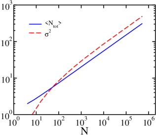
Figure 3: Fluctuations in the total number of clusters. Shown are the average number of clusters, $\langle N_{\rm tot}\rangle$ and the variance, $\sigma^{2}=\langle N_{\rm tot}^{2}\rangle-\langle N_{\rm tot}\rangle^{2}$ for $\lambda=0.5$.

To quantify fluctuations in the total number of polymers, we also measured the variance $\sigma^{2}=\langle N_{\rm tot}^{2}\rangle-\langle N_{\rm tot}\rangle^{2}$. We find that the fluctuations follow a central-limit like behavior $\sigma^{2}\sim\langle N_{\rm tot}\rangle$ (figure 3) and therefore,

$$\sigma^{2}\sim N^{\gamma}\qquad{\rm with}\qquad\gamma=\frac{2\lambda}{\lambda+2}$$ (39)

as in (4).

VI Discussion

In summary, we studied stationary and dynamical properties of reversible polymerization. We found an interesting phase transition involving a thermodynamic phase and a non-thermodynamic phase. When fragmentation is strong, the system is in a thermodynamic phase and the number of polymers is proportional to the system size. The system includes a large number of small polymers. When fragmentation is weak, the system is in a non-thermodynamic phase as the total number of polymers grows sub-linearly with the system size. In this phase, there is a small number of large polymers since the size distribution is power-law. Moreover, the polymer sizes are distributed at all scales. Macroscopic gels may exist as well.

In the thermodynamic phase, the system quickly approaches the steady state. The time-dependent behavior is much richer in the non-thermodynamic phase. The system exhibits a finite-time singularity: large moments of the size distribution diverge at the finite gelation time. At this time, the system nucleates macroscopic gels and the size distribution follows a universal algebraic decay. Past the gelation time, there is a second relaxation stage leading the system to a state where there are two balancing fluxes of mass: aggregation transfers mass from small scales to large scales and fragmentation transfers mass from large scales to small scales. The stationary size distribution is algebraic but the characteristic exponent is not universal.

Even though the aggregation process is described by non-linear terms, the analysis in the non-thermodynamic phase involves linear equations because the aggregation gain term is relevant only at the largest scale. Nevertheless, formation of gels at the largest possible scale (in our case, the system size) is crucial in maintaining a stationary state. Understanding the distribution of macroscopic gels is an open challenge, and our numerical simulations reveal an interesting anomaly with an enhancement of the population of macroscopic gels over the algebraic distribution (25) at the maximal scale.

Missing from our calculations is a finite-size scaling analysis bbckw ; bk ; ks ; bk1 near the phase transition point. Interestingly, the total number of clusters grows sub-linearly, $N_{\rm tot}\sim C(\lambda)\,N^{2/3}$, just below the phase transition point, but linearly just above the phase transition point, $N_{\rm tot}\sim(\lambda-1)N$. Therefore, the amplitude $C(\lambda)$ may very well be divergent, and moreover, there must be an intermediate range of fragmentation rates centered around the critical point with a smooth crossover between the two phases. The width of this transition region should vanish as the system size increases.

Understanding fluctuations is another interesting direction for further research. We find Gaussian fluctuations in the thermodynamic phase and are able to compute the variance $\sigma^{2}=\frac{2}{\lambda}N$ but we are unable to obtain (39) in the non-thermodynamic phase.

Finally, we checked that the same phase transition generally holds as long as the aggregation rate is asymptotically proportional to the molecular weights; for instance, when $K_{ij}=Aij+B(i+j)+C$, a class of models that often arise in polymer chemistry pjf ; rld . A more complete characterization of phase transitions in reversible polymerization is another avenue for future work.

Appendix A Detailed Balance

In this appendix, we demonstrate that the detailed balance equations (2) do not generally have a solution. The size densities $c_{k}$ satisfy

$$\begin{split}K_{11}c_{1}^{2}&=F_{11}c_{2}\\ K_{12}c_{1}c_{2}&=F_{12}c_{3}\\ K_{13}c_{1}c_{3}&=F_{13}c_{4}\\ K_{22}c_{2}^{2}&=F_{22}c_{4}\end{split}$$ (40)

for $k=1,2,3,4$. The dimer density and the trimer density are uniquely expressed in terms of the monomer density,

$$c_{2}=\frac{K_{11}}{F_{11}}\,c_{1}^{2},\qquad c_{3}=\frac{K_{11}}{F_{11}}\,\frac{K_{12}}{F_{12}}\,c_{1}^{3}.$$ (41)

However, there are two expressions for the $4$-mer density

$$c_{4}=\frac{K_{11}}{F_{11}}\,\frac{K_{12}}{F_{12}}\,\frac{K_{13}}{F_{13}}\,c_{1}^{4}\qquad c_{4} =\left(\frac{K_{11}}{F_{11}}\right)^{2}\frac{K_{22}}{F_{22}}\,c_{1}^{4}.$$ (42)

These two are identical only when the aggregation and the fragmentation rates satisfy the constraint

$$\frac{K_{12}}{F_{12}}\,\frac{K_{13}}{F_{13}}=\frac{K_{11}}{F_{11}}\,\frac{K_{22}}{F_{22}}.$$ (43)

Therefore, the detailed balance equations (2) have a solution only for special aggregation and fragmentation rates. The constraint (43) reflects the fact that there are multiple paths between two states of the system. For example, a $4$-mer may be formed by two dimers or by a trimer and a monomer. The detailed balance condition (2) requires that the fluxes between any two states of the system balance along all possible paths. This condition leads to constraints of the type (43). The rates (3) violate the constraint (43) as well as infinitely many other constraints. We conclude that in general, the detailed balance equations are overdetermined — there are infinitely many constraints like (43), and a solution does not necessarily exist.

Appendix B Large-size asymptotics

We analyze the large-size asymptotic behavior of the polymer size-density in the thermodynamic phase by introducing the generating function

$$G(z)=\sum_{k}c_{k}\,e^{kz}.$$ (44)

The generating function obeys the differential equation

$$\frac{(G^{\prime})^{2}}{2}-G^{\prime}=\lambda\,\frac{G-M_{0}e^{z}}{1-e^{z}}-\frac{\lambda(G-G^{\prime})}{2}$$ (45)

where ${}^{\prime}\equiv\frac{d}{dz}$ as follows from (5). Next, we shift the generating function by the total density

$$G(z)=M_{0}+F(z),$$ (46)

where $M_{0}$ is given by (7). With this transformation, the differential equation (45) becomes

$$(F^{\prime})^{2}-(2+\lambda)F^{\prime}+1-\lambda+\lambda F\,\frac{e^{z}+1}{e^{z}-1}=0.$$ (47)

By solving this quadratic equation for $F^{\prime}$ we find

$$F^{\prime}(z)=1+\frac{\lambda}{2}-\sqrt{\Phi(z)}$$ (48)

with the shorthand notation

$$\Phi(z)=\frac{1}{4}\,\lambda^{2}+2\lambda-\lambda F(z)\,\frac{e^{z}+1}{e^{z}-1}.$$ (49)

The asymptotic behavior of the size density follows from the singular behavior of the generating function. For instance, the asymptotic behavior

$$c_{k}\simeq Ak^{-\alpha}\,e^{-ak}$$ (50)

implies that the generating function has the following expansion

$$G(z)=G(a)+G^{\prime}(a)(z-a)+A\Gamma(1-\alpha)(a-z)^{\alpha-1}+\ldots$$ (51)

when $z\to a$. Here, it is implicitly assumed that $2<\alpha<3$. By differentiating this equation and by using $G^{\prime}=F^{\prime}$, we further obtain

$$F^{\prime}(z)=F^{\prime}(a)+A\Gamma(2-\alpha)(a-z)^{\alpha-2}.$$ (52)

We now choose $a$ to be the root of $\Phi(z)$, $\Phi(a)=0$, and as a result, equation (48) becomes

$$F^{\prime}(z)=1+\frac{\lambda}{2}-\sqrt{-\Phi^{\prime}(a)}\,(a-z)^{1/2}+\ldots$$ (53)

when $z\to a$. We obtain $F^{\prime}(a)=1+\lambda/2$ by matching the regular terms in (52) and (53), and

$$\alpha=5/2,\quad A\Gamma(-1/2)=-\sqrt{-\Phi^{\prime}(a)}$$ (54)

by matching the singular terms. Therefore, the asymptotic behavior is (9).

The amplitude $A$ can be expressed in terms of $\Phi^{\prime}(a)$. Differentiation of equation (49) yields

$$\Phi^{\prime}(z)=-\lambda\left[F^{\prime}(z)\,\frac{e^{z}+1}{e^{z}-1}-2F(z)\,\frac{e^{z}}{(e^{z}-1)^{2}}\right].$$ (55)

We next set $z=a$ and use

$$F^{\prime}(a)=1+\frac{\lambda}{2}\,,\qquad 2F(a)\,\frac{e^{a}+1}{e^{a}-1}=4+\frac{\lambda}{2},$$ (56)

that follows from (49) and $\Phi(a)=0$ to obtain

$$\Phi^{\prime}(a)=-\frac{\lambda}{2}\left[(2+\lambda)\,\frac{e^{a}+1}{e^{a}-1}-(8+\lambda)\,\frac{e^{a}}{e^{2a}-1}\right].$$ (57)

By using equations (54) and (57) together with the identity $\Gamma(-1/2)=-2\Gamma(1/2)=-\sqrt{4\pi}$ we obtain a relation between the amplitude $A$ and the constant $a$,

$$A=\sqrt{\frac{\lambda}{8\pi}\,\frac{e^{a}+1}{e^{a}-1}\left[2+\lambda-(8+\lambda)\,\frac{e^{a}}{(e^{a}+1)^{2}}\right]}.$$ (58)

In particular, $A\simeq\sqrt{3/(16\pi a)}$, when $\lambda\to 1$.

Appendix C Extremely strong fragmentation

The leading asymptotic behavior in the strong fragmentation limit, $\lambda\to\infty$, can be obtained analytically. The steady state equation (5) shows that $c_{1}=1+O(\lambda^{-1})$ and $c_{2}=\lambda^{-1}+O(\lambda^{-2})$, and that in general,

$$c_{k}\simeq\left(\frac{2}{\lambda}\right)^{k-1}h_{k}$$ (59)

when $\lambda\to\infty$.

To leading order, this form is consistent with the governing equation (5) when the coefficients $h_{k}$ satisfy the recursion equation

$$(k-1)h_{k}=\frac{1}{2}\sum_{i+j=k}ijh_{i}h_{j}.$$ (60)

The first two coefficients are $h_{1}=1$ and $h_{2}=1/2$. We solve this recursion using the generating equation $H(z)=\sum_{k}kh_{k}e^{kz}$. Next, we multiply (60) by $ke^{kz}$ and sum over all $k$ to find that the generating function satisfy the nonlinear differential equation

$$H^{\prime}-H=HH^{\prime}.$$ (61)

We now integrate this equation and find the implicit solution $He^{-H}=e^{z}$. The explicit solution

$$H(z)=\sum_{k=1}^{\infty}\frac{k^{k-1}}{k!}\,e^{kz}$$ (62)

follows from the Lagrange inversion formula wilf . Therefore, the coefficients are $h_{k}=k^{k-2}/k!$ and the leading asymptotic behavior is (10). The large-size asymptotic behavior

$$c_{k}=\frac{e}{\sqrt{2\pi}}\,k^{-5/2}\left(\frac{2e}{\lambda}\right)^{k-1},$$ (63)

when $k\gg 1$, obtained using the Stirling formula $n!\sim\sqrt{2\pi n}n^{n}e^{-n}$, is consistent with the generic asymptotic behavior (9).