MHD simulations of disk-star interaction

Abstract

We discuss a number of topics relevant to disk-magnetosphere interaction and how numerical simulations illuminate them. The topics include: (1) disk-magnetosphere interaction and the problem of disk-locking; (2) the wind problem; (3) structure of the magnetospheric flow, hot spots at the star’s surface, and the inner disk region; (4) modeling of spectra from 3D funnel streams; (5) accretion to a star with a complex magnetic field; (6) accretion through 3D instabilities; (7) magnetospheric gap and survival of protoplanets. Results of both 2D and 3D simulations are discussed.

1 Introduction

Disk accretion to a rotating star with a dipole magnetic field has been investigated theoretically by a number of authors (e.g., Ghosh and Lamb 1978; Camenzind 1990; Königl 1991; Ostriker and Shu 1995; Lovelace, Romanova & Bisnovatyi-Kogan 1995). Recently a number of numerical simulations have been performed assuming axisymmetry (e.g., Hayashi, Shibata & Matsumoto 1996; Miller & Stone 1997; Goodson et al. 1997; Fendt & Elstner 2000; Matt et al. 2002; von Rekowski & Brandenburg 2003; Yelenina, Ustyugova & Koldoba 2006). In some of them, accretion through funnel streams has been clearly observed and investigated (e.g., Romanova et al. 2002; Long, Romanova & Lovelace 2005; Bessolaz et al. 2007, 2008; Zanni, Bessolaz & Ferreira 2007). Full three-dimensional (3D) MHD simulations have been done by Romanova et al. (2003, 2004), for which a special Godunov-type MHD code based on the “cubed sphere” grid has been developed (Koldoba et al. 2002). Longer 3D simulations have been done by Kulkarni & Romanova (2005) and for accretion to a star with a non-dipole magnetic field by Long, Romanova & Lovelace (2007, 2008). Accretion through 3D instabilities has been recently observed in 3D simulations (Romanova, Kulkarni & Lovelace 2007; Kulkarni & Romanova 2008). Spectral lines from 3D funnel streams were calculated by Kurosawa, Romanova & Harries (2008) where a 3D radiative transfer grid has been projected onto the 3D MHD grid. A magnetospheric gap may stop the inward migration of protoplanets at the CTTSs stage (Lin, Bodenheimer & Richardson 1996), unless different processes increase the density inside the gap (Romanova & Lovelace 2006). We discuss these topics in greater detail in the following sections.

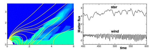
Figure 1: Axisymmetric simulations of winds in the case where the field lines are gathered in an x-type configuration. Left panel shows the distribution of matter flux $\rho v$ and sample field lines. Right panel shows temporal evolution of the accretion rate to the star and to the wind, integrated over the $r=6$ surface. Time is measured in rotational periods at $r=1$. From Romanova et al. (2008).

2 Disk-magnetosphere interaction and disk-locking

Disk-magnetosphere interaction through the closed field lines and through the funnel stream. The accretion disk is disrupted by the stellar magnetosphere and is stopped at the distance $R_{m}$ from the star where the magnetic pressure is approximately equal to the total matter pressure: $B^{2}/8\pi=p+\rho v^{2}$ (e.g., Ghosh & Lamb 1978; see also results of 2D and 3D simulations, Romanova et al. 2002, 2003; Long, Romanova & Lovelace 2005). Matter of the disrupted disk accumulates near $R_{m}$ and is lifted out of the equatorial plane into a “funnel stream” by the pressure gradient force. The matter then follows the star’s dipole field lines and is accelerated by gravity until it hits the star’s surface (Romanova et al. 2002; 2003; Zanni et al. 2007; Bessolaz et al. 2007). Initially, the angular momentum is carried by the funnel stream matter, but later it is converted to angular momentum carried by the field, so that when funnel matter arrives to the surface of the star, almost all angular momentum is carried by magnetic field lines and only few percent by matter (Ghosh & Lamb 1978, 1979; see simulations by Romanova et al. 2002; Long at el. 2005). Whether a star spins-up or spins-down is determined by the ratio between the magnetospheric radius $R_{m}$ and the co-rotation radius $R_{cr}=(GM/\Omega_{*}^{2})^{1/3}$/. When the star rotates slowly, and $R_{cr}>R_{m}$, then the disk matter spins it up (see the main case in Romanova et al. 2002; and Zanni et al. 2007; Bessolaz et al. 2007). In this case the inner disk rotates faster than the star, and closed magnetic field lines connecting the star and the disk form a leading spiral which helps to spin up the star. All of the aforementioned numerical simulations show a direct correlation between the accretion rate $\dot{M}$ (at the surface of the star) and the spin-up rate: the higher the accretion rate, the stronger the spin-up. This correlation may result from the increased twist of closed magnetic field lines connecting the inner disk and the star. If the star rotates fast, so that $R_{cr}<R_{m}$, then matter is still pulled to the funnel flow by gravity, but the star spins down (see e.g., Fig. 6 of Long et al. 2005 for large ¯) because closed field lines form a trailing spiral, so that the star loses angular momentum. We have evidence from simulations that a significant part of the disk-magnetosphere interaction occurs through closed field lines connecting the star and the disk. Opening of external field lines does not lead to disconnection of the star from the disk.

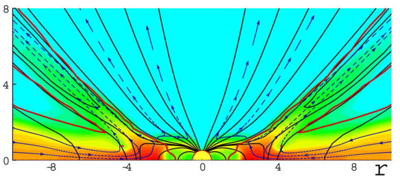
Figure 2: Axisymmetric simulations of a star in the propeller regime. The background shows the density, the thin solid lines are the magnetic field lines, the thick solid lines show the $\beta=1$ line (magnetic energy-density dominates in the corona and in the wind region above the disk. The dashed lines show the streamlines of matter flow. From Romanova et al. (2005).

Where does the angular momentum go? Matter of the disk carries significant specific angular momentum, $j_{m}=\Omega(R_{m})R_{m}^{2}$, which is much larger than that of the star, $j_{*}=\Omega(R_{*})R_{*}^{2}$, if the angular velocities are comparable, $\Omega(R_{m})\sim\Omega(R_{*})$. The question is whether all the angular momentum of the disk, which is carried initially by matter, goes to the star, or whether a significant part of it returns to the disk via the magnetic field, as suggested by Ostriker & Shu (1995). Numerical simulations have not given a final answer to this question yet, but the last possibility appears probable. In this case angular momentum should be constantly removed from the disk by viscosity, some type of waves propagating through the disk, or by winds. X-type winds may be an efficient mechanism of angular momentum removal from inner regions of the disk (Shu et al. 1994) or, winds may flow from the disk at any distance (Pudritz & Norman 1986; Lovelace, Romanova & Bisnovatyi-Kogan 1995; Lamzin et al. 2004; Ferreira, Dougados & Cabrit 2006). If angular momentum does not return back to the disk, then the star will spin up and other mechanisms are required to spin it down. This question needs further investigation.

Inflation of field lines and spinning-down. Differential rotation between the star and the disk leads to the inflation of field lines (Aly 1980; Shu et al. 1994; Lovelace, et al. 1995). Some field lines are strongly inflated and do not transport information between the star and the disk. Other field lines are only partially open and may transport angular momentum between the star and the disk (e.g., the “dead zone” of Ostriker and Shu 1995). Field lines may be only partially open because, for example, the magnetic pressure force leading to opening is balanced by the magnetic tension force opposing the opening. In addition, inflated field lines may reconnect and then inflate again, so that the magnetosphere may not be stationary, but may experience quasi-periodic or episodic restructuring (e.g. Aly & Kuijpers 1990; Uzdensky 2002). Strongly inflated field lines connect the star with the slowly rotating corona, so that angular momentum always flows out from the star to corona. The corona has a low density and is probably magnetically dominated, so that angular momentum may flow from the star to the corona due to the magnetic stress, $\dot{L}_{f}=\int{dS\cdot rB_{\phi}B_{p}/4\pi}$. A star may also lose angular momentum due to major matter outflow from its surface or due to re-direction into the outflow of some of the matter coming to the star through the funnel flow (Matt & Pudritz 2005) where a Weber & Davis (1967) type of angular momentum loss is investigated. In these models it is important to understand the force which lifts the matter (up to 10% of the accretion rate) from the vicinity of the star. Compared to the “material” wind of Matt & Pudritz (2005), the angular momentum carried by the magnetic stress does not require much matter flowing from the star and does not require dense matter in the corona. Estimations show that only $n=10^{5}1/cm^{3}$ are required to support a current associated with twist of magnetic field lines. Thus, angular momentum always flows to the “magnetic tower” (see also Lynden-Bell 2003) and the torque depends on the magnetic field strength and angular velocity of the star. In Long et al. (1995), matter dominates in most of the corona, and spin-down through open field lines does depend on the coronal density. However in the propeller regime (Romanova et al. 2005; Ustyugova et al. 2006), the corona is magnetically-dominated and a significant torque is associated with magnetic tower.

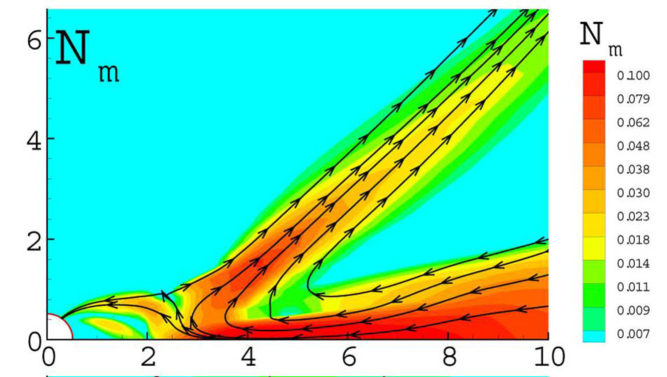
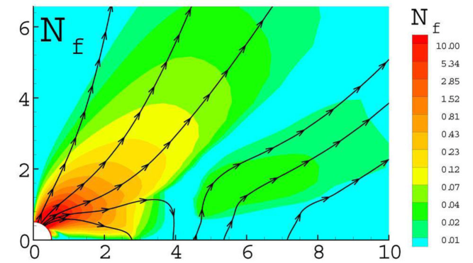
Figure 3: The background shows torques associated with matter $N_{m}$ and the magnetic field $N_{f}$ in the propeller regime. The streamlines show the direction of the angular momentum flow). From Romanova et al. (2005).

Rotational equilibrium state and disk-locking. If a magnetized star accretes for a sufficiently long time, it is expected to be in the rotational equilibrium state, that is when the total positive spin acting on the star equals the total negative spin. Many CTTSs are expected to be in the rotational equilibrium state (Bouvier 2007). If $R_{m}=R_{cr}$, then both inflated and partially-open field lines (which thread the disk at $r>R_{cr}$) will lead to spin-down of the star. So in the rotational equilibrium state, $R_{cr}=kR_{m}$, where $k>1$. Numerical simulations have shown that $k=1.2-1.5$ (Romanova et al. 2002; Long et al. 2005). However in both cases matter dominates in the corona and this led to quite large angular momentum outflows associated with inflated and partially open field lines. In the best cases of Long et al. (2005) the coronal density is $3\times 10^{-4}$ of that in the disk. If the corona above the disk has this density (say, due to winds from the disk or the star) then the estimations done in this paper are correct.

3 Modeling of jets and winds from CTTSs

Jets and winds are observed from a number of CTTSs (e.g Cabrit et al. 2007). In some cases only slow jets are observed Brittain et al. 2007). Clear outflow signatures are also seen as absorption features in the blue wings of some lines, such as the He I line which shows outflow of the order of up to 10% of the disk mass (Edwards et al. 2003; Kwan et al. 2007; see also Hartmann 1998).

Winds from slowly rotating stars. In early simulations of slowly rotating stars we did not observe any significant outflows from the disk or from the disk-magnetosphere boundary (Romanova et al. 2002, Long et al. 2005). It is clear that an x-type configuration is favorable for launching outflows from the disk-magnetosphere boundary (Shu et al. 1994). To obtain this configuration, we suggested that the accretion rate is initially low but later increases, and matter comes to the simulation region bunching field lines into an x-type configuration. In addition we suggested that the $\alpha-$ parameters regulating viscosity, $\alpha_{v}$, and diffusivity, $\alpha_{d}$, are not very small, $\alpha_{d}=0.1$ (compared to earlier research, where we typically chose $\alpha\approx 0.02$. In addition, we chose the viscosity to be several times larger than the diffusivity, so that the bunching of field lines would be supported by the flow. An increase of $\alpha_{d}$ from 0.02 to 0.1 helped obtain a reasonable rate of penetration of incoming matter through field lines. In this case we obtained a quasi-periodic, x-type wind (see an example of simulations in Fig. 1, where $\alpha_{d}=0.1$ and $\alpha_{v}=0.3$). We observed multiple outbursts of matter into the wind, driven by a combination of magnetic and centrifugal forces (Romanova et al. 2008, in preparation). Typical velocities in the outflow are $v=30-60km/s$, for typical parameters of CTTS and up to $20\%$ of the disk matter flows to the wind. The simulations run long, about $800$ rotations at $r=1$. Similar conical x-type outflows have recently been observed with more general initial conditions. It looks like some outflows are also observed by Bessolaz et al. (2007) and Zanni et al. (2007). We should note that in their runs diffusivity is even higher. It seems that relatively high diffusivity is a necessary condition for getting outflows from the disk-magnetosphere boundary.

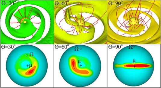
Figure 4: 3D simulations of accretion to a star with a misaligned dipole magnetic field at misalignment angles $\Theta=30^{\circ}$, $\Theta=60^{\circ}$, $\Theta=90^{\circ}$. Top panels show matter flow in the inner part of the simulation region and magnetic field lines. Bottom panels show corresponding hot spots on the surface of the star, where the color background shows kinetic energy density. From Romanova et al. (2004).

Winds from rapidly rotating stars. If $R_{m}>R_{cr}$ then the star is in the “propeller” regime (e.g., Illarionov & Sunyaev 1975; Lovelace, Romanova & Bisnovatyi-Kogan 1999). This regime may occur if the accretion rate decreases, causing $R_{m}$ to increase. Or, it may be a typical stage during the early years of the CTTSs evolution. Axisymmetric simulations of the propeller stage have shown that once again, at low diffusivity $\alpha_{dif}=0.02$, there are no outflows, while at larger diffusivity, $\alpha_{dif}>0.1$, conical quasi-periodic or episodic outflows form and carry away a significant part of the disk matter as wind (see Fig. 2, also Romanova et al. 2005; Ustyugova et al. 2006). Fig 3 (left panel) shows that a significant part of the angular momentum carried by matter is redirected into conical outflows. Fig 3 (right panel) shows that large part of the angular momentum flows into the corona along the open magnetic field lines (through the magnetic tower) and some flows from the disk to the corona. In the propeller regime we were able to obtain a magnetically-dominated corona, and Fig. 3 shows an example in which the star loses about half of its angular momentum through the magnetic wind. The propeller stage may be important in fast spin-down of young CTTSs.

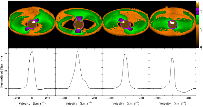
Figure 5: Pa$\beta$ model intensity maps (upper panels) and the corresponding profiles (lower panels) computed at rotational phases $t=0.0$, $0.25$, $0.5$ and $0.75$ (from left to right) and for inclination $i=60^{\circ}$. The misalignment angle of the magnetic axis is fixed at $\Theta=15^{\circ}$. The intensity is shown on a logarithmic scale with an arbitrary units. From Kurosawa et al. (2008).

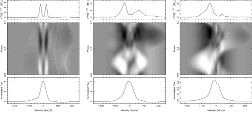
Figure 6: The summary of the Pa$\beta$ spectra computed for the MHD model with $\Theta=15^{\circ}$ and $i=10^{\circ},60^{\circ}$ and $80^{\circ}$ respectively from left to right. The spectra were computed at $50$ different rotational phases. In the bottom panels, the mean spectra of all rotational phases are shown. In the middle panels, the quotient spectra (each spectrum divided by the mean spectrum) are shown as grayscale images with increasing rotational phases in the upward vertical direction. The temporal variance spectra $(\mathrm{TVS})^{-1/2}$ are shown in the top panels. From Kurosawa et al. (2008).

4 Properties of the funnel streams, hot spots and the inner disk

A wide variety of different features were found in our full 3D MHD simulations of disk accretion to a rotating magnetized star with a misaligned dipole magnetic field (Romanova et al. 2003, 2004). Simulations were done for a variety of misalignment angles from $\Theta=0^{\circ}$ to $\Theta=90^{\circ}$, where $\Theta$ is the angle between the magnetic axis of the dipole $\mu$ and the angular velocity of the star $\Omega$ (which was aligned with the angular velocity of the disk). Below we summarize some interesting features observed in 3D simulations:  (1) 3D simulations have shown that the system becomes noticeably non-axisymmetric even at very small misalignment angles $\Theta\sim 2^{\circ}-5^{\circ}$. Thus, most magnetized stars are expected to be non-axisymmetric and will form funnel flows and non-axisymmetric hot spots. (2) Matter accretes to the star through funnel streams which are not homogeneous. The density is largest in the interior regions of the stream, and decreases outwards, so that the appearance of the streams depends on the density: at the largest densities they look like thin streams. At lower densities the stream is wider. The matter covers the whole magnetosphere at the lowest densities.  (3) There are usually two streams which flow to the nearest poles. Some matter flows to the further pole which often leads to a second, weaker set of streams. In the case of high $\Theta$, one wide stream often splits into two streams.  (4) The structure of the hot spots reflects the structure of the funnel streams: the density and specific kinetic energy are larger in the central regions of spots. Thus, hot spots are “hotter” in the center, and cooler outside. They have different shapes, ranging from bow-shaped for small misalignment angles to bar-shaped for large misalignment angles (see Fig. 4).  (5) Variability curves from the hot spots obtained from numerical simulations for different misalignment angles $\Theta$ and different inclination angles $i$ of the disk show a variety of shapes, which may be used to constrain $\Theta$ and $i$.  (6) The density distribution in the disk around the magnetized star is inhomogeneous. It has always a shape of spirals (see Fig. 4.  (7) The inner regions of the disk are slightly warped which reflects the tendency of matter to flow in the magnetic equatorial plane. This warped disk may obscure the light from the star, and this may lead to quasi-periodic variations of light (Bouvier et al. 2003).

Figure 7: 3D simulations of accretion to a star with aligned dipole plus quadrupole fields. Both dipole and quadrupole magnetic moments are misaligned relative to the rotation axis at $\Theta=30^{\circ}$. Here $B_{dipole}\approx 0.45B_{quad}$. From Long et al. (2007).

5 Radiative transport and calculation of spectral lines

We calculated the line profiles from 3D funnel streams using the radiative transfer code TORUS (Harries 2000; Kurosawa et al. 2004, 2005, 2006; Symington et al. 2005) which was modified to incorporate the density, velocity and gas temperature structures from the 3D MHD simulations (Romanova et al. 2003, 2004). The radiative transfer code uses a three-dimensional (3D) adaptive mesh refinement (AMR) grid. We take 3D MHD simulations which come to quasi-stationary state, take parameters of the flow for some moment of time and calculate spectrum from the funnel streams using TORUS code.

We study the dependence of the observed line variability on two main parameters: (1) the inclination angle ($i$) and (2) the misalignment angle ($\Theta$). Here, we show sample results for $\Theta=15^{\circ}$. As $\Theta$ is rather small, the accretion occurs in two arms, creating two hot spots on the surface of the star (Romanova et al. 2004; see also Fig. 4). As one can see from Fig. 5 ($i=60^{\circ}$)the largest amount of red wing absorption occurs at the rotational phase at which a hot spot is facing the observer and when the spot-funnel-observer alignment favorable.

The line variability behavior is summarized in Fig. 6 which shows the phase averaged spectra, the quotient spectra as a function of rotational phase (in the gray scale images), and the temporal variance spectrum (TVS), which is similar to the root-mean-square spectra (c.f. Fullerton, Gies, & Bolton 1996; Kurosawa et al. 2005). The mean spectra of three models are fairly symmetric about the line center; however, a very weak but noticeable amount of absorption in the red wings can be seen in the spectra at all $i$. For $i=10^{\circ}$ and $60^{\circ}$ cases, the flux levels in their red wing become slightly below the continuum level, but the level remains above the continuum for $i=80^{\circ}$ case. Although the line equivalent width of the mean spectra for $i=10^{\circ}$ is slightly smaller than that of the $i=60^{\circ}$ and $80^{\circ}$ cases, no major difference is seen between the three models.

In general, the line profile shapes and strength predicted by the radiative transfer model based on the MHD simulations are similar to those seen in the atlas of the observed Pa$\beta$ and Br$\gamma$ given by Folha & Emerson (2001). The level of the line variability seen in the time-series spectroscopic observation (Pa$\beta$) of SU Aur (Kurosawa et al. 2005, see their Fig. 1) is comparable to our models, Fig. 6). The double-peaked variability pattern (TVS) seen in the low inclination angle model (i.e. $i=10^{\circ}$ model in Fig. 6) is very similar to that of H$\alpha$ and H$\beta$ from the CTTS TW Hydra observed by Alencar & Batalha (2002). The system has a low inclination angle ($i=18^{\circ}\pm 10^{\circ}$, Alencar & Batalha 2002) which is consistent with our model ($i=10^{\circ}$). Although not shown here, the line variability predicted from a model with $i=75^{\circ}$ and $\Theta=60^{\circ}$ resembles that of H$\beta$ from CTTS AA Tau observed by Bouvier et al. (2007). More careful analysis and tailored model fits of observations are required for deriving fundamental physical parameters of a particular system.

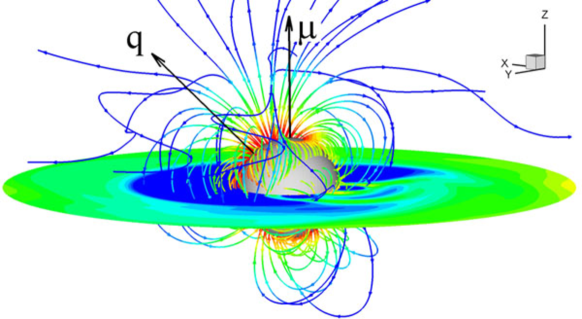
Figure 8: 3D simulations of accretion to a star with a complex magnetic field: a combination of a dipole moment along the z-axis and a quadrupole moment misaligned at $\chi=45^{\circ}$. The equatorial slice shows the density distribution. From Long et al. (2008).

6 Accretion to a star with a complex magnetic field

The magnetic field of a young T Tauri star may have a complex structure (see e.g. Johns-Krull et al. 1999; Smirnov et al. 2003; Gregory, et al. 2006; Jardine et al. 2006). Observational properties of magnetospheric accretion lead to the conclusion that the magnetic field of many CTTSs may consist of a combination of dipole and multipole fields (e.g., Bouvier et al. 2007). If a star has several magnetic poles, then matter may flow to the star in multiple streams, choosing the shortest path to the nearby pole. Some magnetic poles are expected to be closer to the equator of the star compared with the pure dipole case. The observational properties of hot spots will also be different. A picture of matter flow to a star with a complex magnetic field (deduced from Doppler tomography, e.g. Jardine et al. 2006) has been calculated by Gregory et al. (2006). It was shown that matter accretes through several funnel streams choosing, the nearby magnetic poles to accrete.

Recently we were able to perform the first 3D MHD simulations of accretion to a star with a combination of the dipole and quadrupole magnetic fields (Long, Romanova & Lovelace 2007, 2008). Simulations of accretion to a star with a pure quadrupole field have shown that most of the matter flows to the star through the quadrupole “belt”, forming a ring-shaped hot spot at the magnetic equator. In the case of a dipole plus quadrupole field, the magnetic flux in the northern hemisphere is larger than that in the southern hemisphere and the quadrupole belt and the ring are displaced to the south. Fig. 7 shows the case when the magnetic moment of the dipole ¯ and that of the quadrupole $\mathbf{D}$ are aligned and both are misaligned relative the the rotational axis $\mathbf{\Omega}$ at an angle $\Theta$. One can see that the disk is disrupted by the dipole component of the field but the quadrupole component is strong enough to guide matter streams to the poles. At different $\Theta$ the light curves have a variety of different features, but many of these features are observed in the pure dipole cases at somewhat different $\Theta$ and inclination angle of the system $i$. So, it would be challenging to deduce the magnetic field configuration from the light curves (Long et al. 2008).

As the next step we investigated accretion to a star with a dipole plus quadrupole field, when the magnetic axis of the quadrupole is misaligned relative to magnetic axis of the dipole at an angle $\chi$ (Long et al. 2008). Fig. 8 shows an example of such a accretion for $\chi=45^{\circ}$.

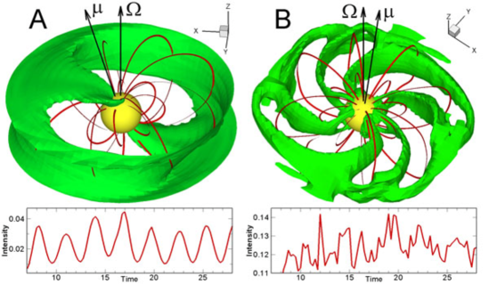
Figure 9: Left panel: in stable accretion matter accretes in two ordered funnel streams and the light-curve has an ordered, almost sinusoidal shape. Right panel: in the unstable regime matter accretes through multiple tongues and the light-curve is irregular. From Romanova, Kulkarni & Lovelace (2008).

7 Accretion through instabilities

Recent 3D simulations have shown that in many cases, disk matter accretes to the star through a 3D Rayleigh-Taylor instability (Romanova & Lovelace 2006; Romanova, Kulkarni & Lovelace 2008; Kulkarni & Romanova 2008). Penetration of matter through 3D instabilities has been predicted theoretically (e.g., Arons & Lea 1976) and has been observed in 2D simulations by Wang & Robertson (1985). In the unstable regime, matter accretes through the magnetosphere forming transient but frequently appearing equatorial tongues (see Fig. 9, right panel). The tongues penetrate deep into the magnetosphere and deposit material onto the star much further away from the magnetic poles than funnel streams do. The structure of the tongues is opposite to that of the magnetospheric funnel streams: they are narrow in the longitudinal direction, but wide in latitude (see Fig. 9). The number and location of the tongues varies with time. The number varies between $m=2$ and $m=7$ and depends on parameters of the model. For example, $m=2$ dominates if the misalignment angle of the dipole is not very small, $\Theta\sim 15^{\circ}-30^{\circ}$. The tongues hit the surface of the star and form randomly distributed hot spots, so that the light curve looks irregular. In some cases quasi-periodic oscillations are observed when a definite number of tongues dominates. Simulations have shown that this type of accretion occurs in cases when the accretion rate is relatively high (Romanova et al. 2008; Kulkarni & Romanova 2008).

8 Magnetospheric gaps and survival of protoplanets

A young star with a strong dipole magnetic field is surrounded by a low-density magnetospheric gap where planets may survive longer than in the disk, due to the low density of matter inside the gap (if their orbit is inside the 2:1 resonance with the inner radius of the disk) (Lin et al. 1996; Romanova & Lovelace 2006; see sketch at the Figure 10). For typical CTTS the inner edge of the truncated disk approximately coincides with the peak in distribution of close-in planets ($P\approx 3days$). We investigated in 3D simulations the emptiness of magnetospheric gaps in different situations.

Magnetospheric gaps around stars with a dipole magnetic field. We observed from 3D simulations that in case of the dipole field and relatively small misalignment angles, $\Theta<30^{\circ}$, the magnetospheric gap has quite a low density (see Figure 10, right panel). However, for sufficiently large $\Theta$, $\Theta>45^{\circ}$, part of the funnel stream crosses the equatorial plane, so that magnetospheric gap is not empty (Romanova & Lovelace 2006).

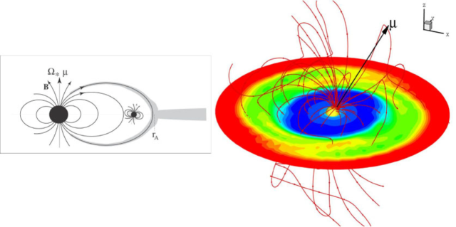
Figure 10: Left panel: sketch of the magnetospheric gap. Right panel: result of 3D MHD simulations, where dark blue shows low density, and red - high density with a contrast of 300. Red lines are sample magnetic field lines. From Romanova & Lovelace (2006)

Magnetospheric gaps around stars with complex magnetic fields. The magnetic field of a young T Tauri star may have a non-dipole, complex structure (see e.g. Gregory, et al. 2006). If the dipole component dominates at large distances, and other components of the field are weaker multipoles, then a magnetospheric gap may form, as in the case of the dipole field (e.g., Bouvier et al. 2007). However, if multipoles are sufficiently strong compared with the dipole field, then matter may accrete through several streams and will chose a path to the nearby poles which are closest to the equatorial plane. In this situation some of funnels may cross the equatorial plane and increase the density in the magnetospheric gap (see example in Fig. 8).

Accretion through 3D instabilities and magnetospheric gaps. At sufficiently high accretion rates in the disk matter accretes to the star through 3D instabilities (e.g., Romanova et al. 2008; Kulkarni & Romanova 2008, see Fig. 9, right panel) and the magnetospheric gap is not empty. Such accretion is expected at the early stages of evolution of the CTTSs, when the accretion rate is expected to be higher. Probably, at this early stage many protoplanets form, migrate inward, and are absorbed by the star.