A model of HIV budding and self-assembly, role of cell membrane

Abstract

Budding from the plasma membrane of the host cell is an indispensable step in the life cycle of the Human Immunodeficiency Virus (HIV), which belongs to a large family of enveloped RNA viruses, retroviruses. Unlike regular enveloped viruses, retrovirus budding happens concurrently with the self-assembly of retrovirus protein subunits (Gags) into spherical virus capsids on the cell membrane. Led by this unique budding and assembly mechanism, we study the free energy profile of retrovirus budding, taking into account of the Gag-Gag attraction energy and the membrane elastic energy. We find that if the Gag-Gag attraction is strong, budding always proceeds to completion. During early stage of budding, the zenith angle of partial budded capsids, $\alpha$, increases with time as $\alpha\propto t^{1/3}$. However, when Gag-Gag attraction is weak, a metastable state of partial budding appears. The zenith angle of these partially spherical capsids is given by $\alpha_{0}\simeq(\tau^{2}/\kappa\sigma)^{1/4}$ in a linear approximation, where $\kappa$ and $\sigma$ are the bending modulus and the surface tension of the membrane, and $\tau$ is a line tension of the capsid proportional to the strength of Gag-Gag attraction. Numerically, we find $\alpha_{0}<0.3\pi$ without any approximations. Using experimental parameters, we show that HIV budding and assembly always proceed to completion in normal biological conditions. On the other hand, by changing Gag-Gag interaction strength or membrane rigidity, it is relatively easy to tune it back and forth between complete budding and partial budding. Our model agrees reasonably well with experiments observing partial budding of retroviruses including HIV.

I Introduction

The Human Immunodeficiency Virus (HIV) is famous for its ability to induce Acquired Immunodeficiency Syndrome (AIDS). It belongs to a large family of enveloped RNA viruses, retroviruses. Retroviruses are characterized by the unique infection strategy of reverse transcription, in which the genetic information flows from RNA back to DNA (therefore the name “retro”) Coffin et al. (1997). Budding is an indispensable step in the retroviral life cycle Morita and Sundquist (2004); Demirov and Freed (2004). After the major retroviral structural protein, Gags, are synthesized inside the host cell, they are transported to the cell membrane and self-assemble into spherical protein shells called “capsids”, with viral RNA genome and other auxiliary viral proteins packaged inside. At the same time, these capsids, enveloped by the cellular membrane, have to bud out of the membrane to target other host cells. In other words, budding and assembly of retroviruses happen concurrently on the cell membrane.

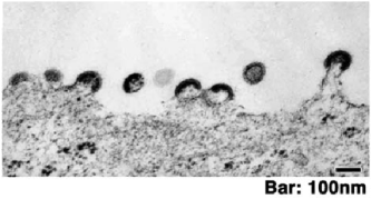
Figure 1: Electron microscopic image of partial budding of HIV-1 viruses (reprinted from Morita and Sundquist (2004)).

Despite a large body of experiments done within the last decade, the biological pathway and mechanism of retroviral budding have still not been fully understood Morita and Sundquist (2004); Demirov and Freed (2004). One important unexplained observation is that viral budding can be inhibited partially or completely by changing the cell environment or mutating the late domains of the Gag proteins. In these situations, capsids are only partially formed and stuck on the membrane (Fig. 1). Motivated directly by this partial budding phenomenon, in this paper, we propose a physical model to study HIV (and retroviruses in general) budding and assembly on the elastic membrane. Physically, this situation is interesting because it provides a unique two dimensional self-assembly mechanism in which the membrane elastic energy plays an important role, since assembly is always accompanied with budding. Biologically, understanding the physical mechanism of HIV budding and assembly is certainly important toward understanding the HIV life cycle. It is also important in the light of recent effort from the virology community to develop assembly-oriented anti-viral therapy.

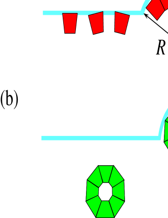
Figure 2: (Color online) Schematic illustrations of two different types of virus budding. (a): budding of retroviruses: capsid proteins (Gags) are first attracted to the membrane, then self-assemble and bud on the membrane at the same time. This is the system studied in this paper. (b): budding of regular enveloped viruses: capsid proteins first self-assemble into complete capsids inside the cell, then bud on the membrane Tzlil et al. (2004). (a) also shows the cylindrical coordinate system $(r,h,\phi)$ used in the model (the polar angle $\phi$ is not shown).

Budding of regular enveloped viruses was studied theoretically by several authors (TDGB) in Ref. Tzlil et al. (2004); Deserno and Bickel (2003); Deserno (2004). However, the viral budding pathway and the physical model studied by TDGB is qualitatively different from retroviral budding we study in this paper. For regular enveloped viruses, viral capsids are fully assembled inside the cell Zlotnick (2007); Hagan and Chandler (2006); Hu and Shklovskii (2007). After that, they are transported to the cell membrane, bind to the viral spike proteins (embedded in the cell membrane) and then bud out through the cell membrane (see Fig. 2b). Therefore, capsids formation and budding out of the membrane are two separate processes. And the main driving force of budding is the capsid-membrane attraction (mediated by embedded spike proteins).

Budding of retroviruses follows a completely different pathway. Various TEM and X-ray tomography experiments suggest that retroviral capsids are assembled from Gag proteins on the cell membrane and bud out of the cell concurrently  Morita and Sundquist (2004); Demirov and Freed (2004). Based on these experiments, we study a different model for HIV (and retrovirus in general) budding and assembly shown in Fig. 2a. In this new model, we assume retroviral capsids are assembled from membrane-bound Gags only, neglecting the possibility that Gags from the interior of the cell may participate. In other words, the Gag-membrane attraction is strong such that Gags always bind to the membrane. This assumption is supported by various experimental observation where budding is completely inhibited (no capsids are formed) but Gags are found in abundance at the cell membrane Dooher et al. (2007) . In contrast to the TDGB model, the primary driving force of our retroviral budding is the short range attraction between these membrane-bound Gag proteins. This correlates well with experimental fact that point mutations changing Gag-Gag interactions affect the degree of viral budding. On the other hands, spike proteins or virus RNA seem not important for retroviral budding. In vitro, Gag proteins are directly attracted to the membrane and they alone are usually sufficient for the assembly and release of virus-like particles Demirov and Freed (2004); Garoff et al. (1998); Welsch et al. (2007). We therefore neglect the contribution of all other proteins or RNA components of retroviruses in our model.

In this paper, for a given set of parameters (the membrane Gag concentration, the Gag-Gag interaction, and the cell membrane bending and stretching rigidity), we study the free energy profile of budded viral capsids. Two energies are considered explicitly: first, the elastic energy of the membrane including the bending and stretching energy; second, the Gag-Gag attraction energy when a Gag makes contact to the other Gag (see Fig. 2a). Since the elastic energy scale is much larger than k_BT, for example, the bending rigidity of normal membranes is about $20$ k_BT, thermal fluctuations are higher order corrections and neglected in the theoretical treatment. Focusing on the budding process, we also assume that the Gag-Gag interaction is strong enough such that the entropic cost of bringing free Gags to the capsid can be ignored. For simplicity, we assume the shape of the capsid together with the membrane attached to it is (partially) spherical with radius $R$ (Fig. 2a). The size of a capsid is then characterized by the zenith angle $\alpha$ at its edge, the smallest being the angle of a single Gag protein, $\alpha_{G}$ (Fig. 2a). Since $\alpha_{G}$ is very small ($\alpha_{G}=0.03$ for a typical HIV capsid containing 5000 Gags), we take $\alpha_{G}\rightarrow 0$ in the theoretical consideration and treat $\alpha$ as a continuous variable. As budding proceeds to completion, $\alpha$ increases from $\alpha_{G}$ to $\pi$. When $\alpha=\pi$, the capsid actually leaves the membrane through membrane fission. In this paper, we do not consider this fission process and thus, in our terminology, complete budding always means $\alpha\rightarrow\pi$. To simplify the calculation, we employ an scaling description where we neglect the variation in the degree of viral budding and assume all capsids have the same average zenith angle $\alpha$.

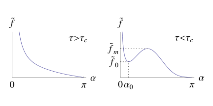
Figure 3: The schematic illustration of the total free energy density as a function of the capsid size $\alpha$. The left and right profiles correspond to strong or weak Gag-Gag attraction respectively. Here $\tau$ is the line tension of the rim of a partially budded capsid. $\tau$ is proportional to the strength of Gag-Gag attraction. $\tau_{c}$ is the threshold line tension at which the local minimum at $\alpha_{0}$ appears.

Our main result is shown in Fig. 3. The key parameter is the strength of Gag-Gag attraction which can be adjusted experimentally by mutating of Gags, complexing of Gags with other molecules or by changing pH or salinity of the cell cytoplasm near the membrane Morita and Sundquist (2004); Campbell et al. (2001). In a partially budded capsid, the line tension $\tau$ of the rim of a capsid is directly proportional to this interaction Gag-gag interaction. When the Gag-Gag attraction is strong (or when $\tau$ is greater than a threshold value $\tau_{c}$), as in the normal biological conditions of HIV, budding always proceeds to completion, i.e., $\alpha\rightarrow\pi$ (the left panel of Fig. 3). At early stage of budding, the size of a partially budded capsid increases very slowly with time:

$$\alpha(t)\approx(t/\tau_{diff})^{1/3}$$ (1)

where the time scale $\tau_{diff}$ depends on the lateral mobility of Gag, the radius of the capsid and the initial concentration Gag (see Eq. (51)). On the other hand, when the Gag-Gag attraction is weak ($\tau<\tau_{c}$), for example, after mutation of the late domains of the Gag protein, partial budding appears as a metastable state at the capsid size $\alpha_{0}$ (the right panel of Fig. 3). In this case, the free energy barrier can be much larger than $k_{B}T$ and budding is kinetically trapped at $\alpha_{0}$. Using a linear approximation, we find

$$\alpha_{0}\simeq\sqrt[4]{\frac{\tau^{2}}{\kappa\sigma}},$$ (2)

where $\sigma$ and $\kappa$ are the surface tension and bending rigidity of the membrane.

The energetics of HIV budding and assembly is studied both analytically and numerically in this paper. Analytically, the complete scaling behaviors of the free energy density profile in asymptotic limits of “soft” and ”stiff” membranes are calculated (the meaning of ”soft” and ”stiff” membrane will be clear in later sections). In all cases, they agree with the numerical result well. However, the numerical result gives a complete solution to the problem including nonlinear regimes where the analytical result is normally not available. The inequility $\alpha_{0}<0.3\pi$ is found to always hold from the numerical calculation without any approximations.

It is worth to point out that budding in our model can be considered as a consequence of the inhomogeneity of the membrane if one considers Gags as a part of the membrane. In this sense, our work is related to Jülicher and Lipowsky’s works on domain-induced budding of vesicles Jülicher and Lipowsky (1993, 1996). However, in their papers, the inhomogeneity was introduced through two kinds of lipids which do not carry a given curvature like our Gags. Domain-induced budding is a consequence of demixing of these different molecules. As a result, their budding happens in a much larger length scale (comparable to the size of the vesicle) where only two phases coexist, one budded out from the other. While in our case, we consider budding at a much smaller length scale (a typical HIV-1 virus particle is about 130 nm in diameter, which is a hundred times smaller than the size of a host cell) and actually have a multi-phase coexistence since there are more than one capsid on the membrane.

This paper is organized as follows. In Sec. II , we introduce the physical model of HIV budding and assembly. We then discuss the analytical solution to the elastic energy of the membrane in Sec. III and to the total free energy density in Sec. IV. The numerical result is then provided and compared to the analytical results in Sec. V. After we get the complete theoretical result, we discuss budding kinetics and make connections to experiments in Sec. VI. We finally conclude in Sec. VII. In this paper, the term “capsid” is used for both partial and complete spherical shells of viral proteins. The meaning should be clear from the context.

II The elastic model of HIV capsid budding and self-assembly

Let us consider a membrane-capsids system in which the concentration of Gags on the membrane, $c_{G}$, is fixed. We assume all capsids assembled by Gags have the same average zenith angle $\alpha$ (see Fig. 2a), and an average concentration, $n$. $n$ is related with $\alpha$ by the conservation of mass of Gags:

$$n=c_{G}\frac{A(\alpha_{G})}{A(\alpha)}=c_{G}\frac{1-\cos\alpha_{G}}{1-\cos\alpha},$$ (3)

where

$$A(\alpha)=2\pi R^{2}\int_{0}^{\alpha}\sin\theta d\theta=2\pi R^{2}(1-\cos\alpha)$$ (4)

is the area of a capsid with zenith angle $\alpha$, and $\alpha_{G}$ is the zenith angle of a single Gag (see Fig. 2a). Within this average description, it is convenient to think that the whole membrane surface is divided into identical cells, each contains a single capsid. The average size of these approximately circular cells, $d$, is given by the condition

$$\pi(d/2)^{2}n=1.$$ (5)

Generically, the free energy density of the membrane-capsid system can be written as

$$f=n\varepsilon=n(\varepsilon_{m}+\varepsilon_{c}),$$ (6)

where $\varepsilon$ is the free energy of one membrane cell. It includes two parts: the elastic energy of the membrane, $\varepsilon_{m}$, and the capsid energy $\varepsilon_{c}$ coming from the Gag-Gag interaction and the Gag-membrane interaction.

To calculate the elastic energy of the cell membrane, we use the standard Helfrich model Canham (1970); Helfrich (1973) where $\varepsilon_{m}$ is the sum of two contributions from the bending energy and the stretching energy:

$$\varepsilon_{m}=\int dS\left[\frac{\kappa}{2}(2H-C_{0})^{2}+\kappa_{G}K\right]+\int dS\sigma.$$ (7)

Here the integration with the area element $dS$ is taken over the membrane surface. $\kappa$ and $\kappa_{G}$ are the bending rigidity and Gaussian bending rigidity, $H$ and $K$ are the mean and Gaussian curvatures, and $C_{0}$ is the spontaneous curvature of the membrane surface. Using the Gauss-Bonnet theorem, one can show that the total Gaussian curvature of the membrane surface is proportional to the total area of capsids, in the generic case when $\kappa_{G}$ takes different values for the membrane attached to the capsid and the Gag-free membrane. Since the Gag concentration $c_{G}$ in our system is fixed, this term gives a constant in $f$ and can be dropped from further consideration G . For a given Gag concentration $c_{G}$, under our spherical capsid assumption, the shape and the total area of all capsids are fixed. Therefore the total elastic energy of the membrane attached to capsids is also constant, and can also be dropped from consideration. As a result, the $\alpha$-dependent contribution to $\varepsilon_{m}$ comes from the integration over the Gag-free membrane surface only. In this region, we take the spontaneous curvature to be $C_{0}=0$, corresponding to normal lipid bilayer membranes.

In consideration of the single capsid energy $\varepsilon_{c}$, since $c_{G}$ is constant, both the total Gag-membrane interaction energy and the bulk part of the Gag-Gag interaction energy are constant. The only $\alpha$-dependent contribution to $\varepsilon_{c}$ comes from the rim energy of the capsid, due to the fact that the coordination number of Gags on the rim is not as many as Gags inside the capsid. Since the perimeter of the capsid rim with zenith angle $\alpha$ is $2\pi R\sin\alpha$, we set

$$\varepsilon_{c}=\tau 2\pi R\sin\alpha.$$ (8)

The proportionality coefficient $\tau$ can be considered as the “line tension” of the capsid. It is directly proportional to the strength of the Gag-Gag attraction and can be changed experimentally by mutations of Gags or by changing pH or salinity of the cell cytoplasm near the membrane.

To proceed further, we take the “ideal capsids” approximation when the distance between capsids is large and the membrane mediated interaction between them is negligible. Such an effective long-range interaction is possible because the presence of the first capsid may change the deformation of the membrane around the second capsid and provides an effective interacting energy between the two. Qualitatively, this interaction is negligible when the capsid concentration $n$ is small (the quantitative condition will be given in the next section). Under this non-interacting capsids approximation, $\varepsilon_{m}$ comes from the membrane deformation induced by a single capsid.

The calculation procedure to find the free energy profile $f(\alpha)$ is as follows. We first minimize the membrane elastic energy $\varepsilon_{m}$ with respect of all possible membrane shapes for any given capsid size $\alpha$. Here it is convenient to use a cylindrical coordinate system $(r,h,\phi)$ as shown in Fig. 2a (the azimuthal angle $\phi$ is not shown). With our assumption of (partial) spherical capsids, the membrane profile is independent on $\phi$. As a result, one can use either the function $h(r)$ or $r(h)$ to parameterize the membrane. Correspondingly, the mean curvature and the area element can be written as Kreyszig (1991)

$$H(r) = \frac{h^{\prime}(r)^{3}+h^{\prime}(r)+rh^{\prime\prime}(r)}{2r[1+h^{\prime}(r)^{2}]^{3/2}},$$ (9)

$$dS = r\sqrt{1+h^{\prime}(r)^{2}}drd\phi;$$ (10)

$$\mathrm{or}\ \ H(h) = \frac{1+r^{\prime}(h)^{2}-r(h)r^{\prime\prime}(h)}{2r(h)[1+r^{\prime}(h)^{2}]^{3/2}},$$ (11)

$$dS = r(h)\sqrt{1+r^{\prime}(h)^{2}}dhd\phi,$$ (12)

where $h^{\prime}(r)=dh/dr$ and $h^{\prime\prime}(r)=d^{2}h/dr^{2}$ are the first and second derivatives of $h$ with respect to $r$. Similarly, $r^{\prime}(h)=dr/dh$ and $r^{\prime\prime}(h)=d^{2}r/dh^{2}$ are the first and second derivative of $r$ with respect to $h$. Functionally minimizing the membrane energy $\varepsilon_{m}$ with respect to membrane shape $r(h)$ or $h(r)$, one obtains an elastic equation of the membrane shape, similar to the Euler-Lagrange equation derived from the least action principle in the classical mechanics. For the shape parametrization using $r(h)$, $\delta\varepsilon_{m}/\delta r=0$ leads to the equation:

$$\frac{\kappa}{2r^{2}[1+r^{\prime 2}]^{9/2}}[-r^{\prime 2}-3r^{\prime 4}-3r^{\prime 6}-r^{\prime 8}+rr^{\prime\prime}-3rr^{\prime 4}r^{\prime\prime}-2rr^{\prime 6}r^{\prime\prime}+2r^{2}r^{\prime\prime 2}-11r^{2}r^{\prime 2}r^{\prime\prime 2}-13r^{2}r^{\prime 4}r^{\prime\prime 2}-5r^{3}r^{\prime\prime 3}$$

$$+30r^{3}r^{\prime 2}r^{\prime\prime 3}+4r^{2}r^{\prime}r^{(3)}+8r^{2}r^{\prime 3}r^{(3)}+4r^{2}r^{\prime 5}r^{(3)}-20r^{3}r^{\prime}r^{\prime\prime}r^{(3)}-20r^{3}r^{\prime 3}r^{\prime\prime}r^{(3)}+2r^{3}r^{(4)}+4r^{3}r^{\prime 2}r^{(4)}+2r^{3}r^{\prime 4}r^{(4)}]$$

$$+\sigma\frac{1+r^{\prime 2}-rr^{\prime\prime}}{[1+r^{\prime 2}]^{3/2}}=0,$$ (13)

where $r^{(3)}=d^{3}r/dh^{3}$ and $r^{(4)}=d^{4}r/dh^{4}$ are the third and forth derivatives of $r$ with respect of $h$. This equation has to be solved together with the boundary conditions. On the rim of the partial spherical capsid, the membrane itself and its slope must be continuous. We have

$$h(r)|_{R\sin\alpha}=R\cos\alpha,\ \ h^{\prime}(r)|_{R\sin\alpha}=-\tan\alpha,;$$ (14)

or

$$r(h)|_{R\cos\alpha}=R\sin\alpha,\ \ r^{\prime}(h)|_{R\cos\alpha}=-\cot\alpha.$$ (15)

Far away from the capsid, the membrane becomes flat. we have

$$h^{\prime}(r)|_{\infty}=0$$ (16)

or

$$r^{\prime}(h)|_{\infty}=\infty.$$ (17)

Solving the elastic equation (13) with the boundary conditions, Eq. (15) and (17) (or Eq. (14) and Eq. (16) if $h(r)$ is used), one obtains the membrane shape that minimizes $\varepsilon_{m}$. Substituting this shape into Eq. (7), one obtains the minimal $\varepsilon_{m}(\alpha)$. Putting its value into Eq. (6), one gets the total free energy density profile $f(\alpha)$. In general, the elastic equation, Eq. (13), is highly non-linear and numerical calculations are needed to obtain the exact membrane profile, as shown in Sec. V. However, in certain asymptotic limits, analytical solutions can be obtained which determine the scaling behavior of the system. This is done in the next two sections.

III Asymptotic solutions of the membrane elastic energy

In calculating the free energy profile, the most nontrivial part is to find the minimal $\varepsilon_{m}(\alpha)$, due to the nonlinear elastic equation involved. After the solution is found, it is straightforward to add the other part of the energy $\varepsilon_{c}(\alpha)$ and get $f(\alpha)$. Therefore we focus on the solution of minimal $\varepsilon_{m}$ in this section. Although not solvable in general, the problem do have analytical solutions in asymptotic limits. To a large extent, they determine the analytical behavior of the system, especially the scaling behavior of $\varepsilon_{m}$ with the dimensionless parameter

$$\widetilde{\sigma}=R\sqrt{\frac{\sigma}{\kappa}},$$ (18)

which characterize the relative strength of the surface tension to the bending rigidity.

III.1 The small deformation solution

A typical approach to consider the elastic deformation of the membrane is to take the small deformation approximation which assumes $|\nabla h|\ll 1$ lar . Here we use the notation

$$\nabla=\hat{r}\partial_{r}+\mathbf{\hat{\phi}}\frac{1}{r}\partial_{\phi}$$ (19)

in order to show similarity of the elastic equation to the linearized Poisson-Boltzmann equation later. Expanding with $\nabla h$ and keeping terms of $O(\nabla h)^{2}$ in $\delta\varepsilon_{m}=0$, we reach a linearized elastic equation which can be written as

$$H=\frac{1}{2}\nabla^{2}h,$$

$$\nabla^{2}H-\frac{H}{r_{s}^{2}}=0,$$ (20)

where we have introduced an important length scale in the problem,

$$r_{s}=\sqrt{\frac{\kappa}{\sigma}}.$$ (21)

It is the length scale beyond which the stretching energy becomes more important than the bending energy. Notice that Eq. (20) takes exactly the same form as a linearized Poisson-Boltzmann equation in electrolytes or plasma Landau and Lifshitz (1980). Therefore $r_{s}$ can be interpreted as an elastic screening length, similar to the Debye-Hückel screening radius. The local curvature $H(r)$ induced by the capsid decreases when $r$ increases and becomes exponentially small at projected distance larger than $r_{s}$. This is a typical linear solution of small deformation.

Using boundary conditions Eqs. (14) and (16), the special solution to Eq. (20) is given by

$$h(r) = R\cos\alpha+r_{s}\tan\alpha\frac{K_{0}(r/r_{s})-K_{0}(R\sin\alpha/r_{s})}{K_{1}(R\sin\alpha/r_{s})},$$

$$h^{\prime}(r) = -\tan\alpha\frac{K_{1}(r/r_{s})}{K_{1}(R\sin\alpha/r_{s})},$$ (23)

$$H(r) = \frac{\tan\alpha}{2r_{s}}\frac{K_{0}(r/r_{s})}{K_{1}(R\sin\alpha/r_{s})},$$ (24)

where $K_{0}$ and $K_{1}$ are the zero and first order modified Bessel function of the second kind. At $r\gg r_{s}$, both $K_{0}(r/r_{s})$ and $K_{1}(r/r_{s})$ decay like $\sqrt{r_{s}/r}\exp(-r/r_{s})$, and the deformation becomes exponentially small, as the meaning of $r_{s}$ suggested.

Substituting this solution back to Eq. (7), we get the minimal elastic energy of the membrane

$$\varepsilon_{m}=\pi\kappa\tan^{2}\alpha\frac{R\sin\alpha}{r_{s}}\frac{K_{0}(R\sin\alpha/r_{s})}{K_{1}(R\sin\alpha/r_{s})}.$$ (25)

Notice that this energy is proportional to the dimensionless parameter $\widetilde{\sigma}=R\sqrt{\sigma/\kappa}=R/r_{s}.$ Here the inverse proportion to $r_{s}$ is again a generic feature shared with the theory of Debye-Hückel linear screening Landau and Lifshitz (1980).

The self-consistency of the small deformation approximation is warranted by $|h^{\prime}(r)|<1$, or, according to Eq. (23), $|\tan\alpha|<1$. Therefore this solution is applicable in the whole range of $r$ for $\alpha<\pi/4$ capsids only. On the other hand, at large distances far away enough from the capsid, the deformation of the membrane always becomes small enough such that the small deformation solution is applicable. In this sense, this solution can always serve as a “far-capsid” solution for the membrane shape, although the formula for $\varepsilon_{m}$ in Eq. (25) is not valid in general. It describes the universal decaying behavior of the deformation when the deformation itself becomes small enough. We can formally define a characteristic distance $r_{c}$ through

$$|h^{\prime}(r_{c})|=1,$$ (26)

beyond which the small deformation solution is valid. $r_{c}$ will be useful later when we discuss the complete solution to the problem.

With the small deformation solution in hand, we are now ready to derive a quantitative condition for the ideal capsid approximation introduced in the last section. Clearly, when the average projected distance between capsids, $d_{0}$, is much larger than $r_{s}+2R$, the membrane mediated interaction between capsids is negligible, since the deformations of the membrane by the capsids at distance larger than $r_{s}$ are screened out. In this case, most of the membrane surface is flat, so $d_{0}\simeq d$ (notice that $d$ is measured along the membrane surface which in general is larger than $d_{0}$ measured along $r$ axis). Thus according to Eqs. (3) and (5), the ideal capsids approximation is valid when

$$\frac{d_{0}}{r_{s}+2R}=\frac{2\sin(\alpha/2)}{(r_{s}+2R)\sqrt{\pi c_{G}}\sin(\alpha_{G}/2)}\gg 1.$$ (27)

In this work, we assume $c_{G}$ is small enough and this is always the case.

III.2 The catenoid solution

When the surface tension $\sigma=0$, or, $r_{s}\rightarrow\infty$, again an analytical solution is available kap . In this case, the second integral in Eq. (7) is zero. Our problem of finding the minimal $\varepsilon_{m}$ is reduced to a minimal surface problem in differential geometry Kreyszig (1991). Namely, we look for the solution to the equation $H=0$ H . The only solution under the rotational symmetry of our problem is the catenoid solution, first discovered by Euler in 1740 Morgan (1993).

In this case, due to the possible multiple values of $h$ at the same $r$, it is better to use the $r(h)$ representation. $H$ is then given by Eq. (11). Using boundary conditions (15) and (17), the special solution to $H=0$ is

$$r(h)=R\sin^{2}\alpha$$

$$\quad\cosh\frac{h-R\cos\alpha-R\sin^{2}\alpha\mathop{\mathrm{arcsinh}}(\cot\alpha)}{R\sin^{2}\alpha}.$$ (28)

The catenoid shapes for various $\alpha$ are depicted in Fig.  4. In this catenoid shape, the elastic energy $\varepsilon_{m}$ achieves its absolute minimum, zero.

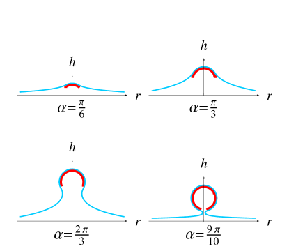
Figure 4: (Color online). In the limit of small surface tension, the optimal membrane shapes (thin line, blue online) around the capsid (thick line, red online) are catenoids, as shown for different capsid sizes.

The catenoid solution is a solution to a nonlinear differential equation. It involves large deformations which can not be characterized by the linear solution discussed in the last subsection. Although exact only when $r_{s}\rightarrow\infty$, this solution is still useful for large but finite $r_{s}$ cat . In fact, since there are no other length scales in the elastic equation (13) ($R$ only shows up in the boundary conditions), a large $r_{s}$ actually means $r_{s}\gg r$. Therefore in the region of $r\ll r_{s}$, the catenoid solution should work asymptotically. In this sense, this solution can always serve as a “near-capsid” solution for the membrane shape, although $\varepsilon_{m}=0$ is not true in general. The characteristic length beyond which it fails is simply $r_{s}$.

In case of $r_{s}\rightarrow\infty$ and $\alpha\ll 1$, both the catenoid solution and the small deformation solution work in all range of $r$. Indeed they become identical.

III.3 Membrane elastic energy at two asymptotic limits

The two solutions discussed in the last two subsections determine the analytical behavior of the system to a large extent. When $\widetilde{\sigma}\ll 1$, they can be combined to get the analytical expression of the minimal $\varepsilon_{m}$. In general, they determine the scaling behavior of $\varepsilon_{m}$ with respect of $\widetilde{\sigma}$. We separate our discussion into two opposite limits of small and large $\widetilde{\sigma}$, which can be called the soft membrane regime and the stiff membrane regime. Here “soft” means easy to stretch, “stiff” means the opposite.

In the soft membrane regime, $\widetilde{\sigma}\ll 1$ or $R\ll r_{s}$, the catenoid solution is valid near the capsid when $r\ll r_{s}$. Calculating $r_{c}$ using Eqs. (28) and (26), we get

$$r_{c}=\sqrt{2}R\sin^{2}\alpha.$$ (29)

We see $r_{c}\ll r_{s}$. Therefore the valid regions of the two asymptotic solutions (one is $r>r_{c}$, the other is $r<r_{s}$) overlap largely and we can combine them to get a complete solution to the optimal membrane shape. Quantitatively, we artificially choose a projected distance somewhere between $r_{c}$ and $r_{s}$, say $\sqrt{r_{c}r_{s}}$. For $r<\sqrt{r_{c}r_{s}}$, the catenoid solution is used. For $r>\sqrt{r_{c}r_{s}}$, the small deformation solution is used. Notice that the special solution of the small deformation has to be calculated using the continuity conditions for $h(r)$ and $h^{\prime}(r)$ at $\sqrt{r_{c}r_{s}}$, derived from the catenoid solution. As a result, we have an analytical expression for the optimal membrane shape continuously from the edge of the capsid to infinity. The corresponding $\varepsilon_{m}$, keeping the leading order terms in the small parameter $\widetilde{\sigma}$, is given by

$$\varepsilon_{m}=\pi\kappa\sin^{4}\alpha\frac{R^{2}}{r_{s}^{2}}\ln\frac{r_{s}}{R}.$$ (30)

When $\alpha\ll 1$, this result agrees with the small deformation solution in Eq. (25) in the same regime of small $\widetilde{\sigma}$. In this limit, we have $\varepsilon\propto\widetilde{\sigma}^{2}\ln(1/\widetilde{\sigma})$.

In the stiff membrane regime, $\widetilde{\sigma}\gg 1$ or $R\gg r_{s}$. Since $r\gg r_{s}$ always, the “near capsid” region where the catenoid solution holds disappears. On the other hand, for $\alpha<\pi/4$, the small deformation solution is valid in the whole range of $r$. The membrane elastic energy is given by (25), which in this limit reads,

$$\varepsilon_{m}=\pi\kappa\tan^{2}\alpha\sin\alpha\frac{R}{r_{s}}.$$ (31)

For $\alpha>\pi/4$ capsids, a rough estimate of $r_{c}$ using Eq. (23) gives

$$r_{c}\simeq R\sin\alpha+r_{s}\ln|\tan\alpha|.$$ (32)

Since $R\gg r_{s}$, for most of $\alpha$, we expect that the small deformation solution starts to work at places close to the capsid. Probably because of this, the scaling behavior of $\varepsilon_{m}\propto\widetilde{\sigma}$ is preserved even at large $\alpha$, as shown by the numerical result (see Sec. V).

IV Analytical result of the total free energy density

After the information about the minimal $\varepsilon_{m}(\alpha)$ is known, we can add the line tension energy $\varepsilon_{c}(\alpha)$ to it and consider the total free energy density $f(\alpha)$. The presence of $\varepsilon_{c}$ introduces the second dimensionless parameter to the problem,

$$\widetilde{\tau}=\frac{R\tau}{\kappa},$$ (33)

which characterize the relative strength of the line tension on the capsid rim. In this section, we derive several simple scaling behaviors of the system, depending on the two dimensionless parameters $\widetilde{\sigma}$ and $\widetilde{\tau}$. We again separate our discussion into the soft and stiff membrane regimes corresponding to small and large $\widetilde{\sigma}$.

IV.1 The soft membrane regime

In the soft membrane regime, $\widetilde{\sigma}=R/r_{s}\ll 1$. Substituting Eqs. (8) and (25) to Eq. (6), we have

$$f \equiv \kappa c_{G}(1-\cos\alpha_{G})\widetilde{f}$$

$$= \kappa c_{G}(1-\cos\alpha_{G})\pi\cot\frac{\alpha}{2}(2\widetilde{\tau}+\widetilde{\sigma}^{2}\ln\frac{1}{\widetilde{\sigma}}\sin^{3}\alpha),$$

where we have introduced the dimensionless free energy density $\widetilde{f}$ for convenience. $\widetilde{f}(\alpha)$ is plotted schematically in Fig. 3. When $\widetilde{\tau}$ is large, the only minimum of the free energy density is at $\alpha\rightarrow\pi$ (the left panel of Fig. 3). On the other hand, when $\widetilde{\tau}<0.2\widetilde{\sigma}^{2}\ln(1/\widetilde{\sigma})$, a local minimum at the capsid size, $\alpha_{0}$, appears ( the right panel of Fig. 3). Correspondingly, the threshold line tension at which the local minimum in the free energy density appears is

$$\tau_{c}=0.2R\sigma\ln\frac{1}{R\sqrt{\sigma/\kappa}}.$$ (35)

Since transcendental equations are involved in minimization of $\widetilde{f}$, it is not easy to get the analytical expression about this local minimum in general. However, $\alpha_{0}$ and the corresponding $\widetilde{f}_{0}$ can be estimated in a linear approximation. Assuming $\alpha_{0}$ is achieved at small $\alpha$, we can expand $\widetilde{f}$ and keep only the leading order terms in $\alpha$. We get

$$\widetilde{f}=\frac{4\pi\widetilde{\tau}}{\alpha}+2\pi\widetilde{\sigma}^{2}\ln\frac{1}{\widetilde{\sigma}}\alpha^{3}.$$ (36)

Taking $\partial f/\partial\alpha=0$, we have

$$\alpha_{0}=\sqrt[3]{\frac{\widetilde{\tau}}{\widetilde{\sigma}^{2}\ln(1/\widetilde{\sigma})}}=\sqrt[3]{\frac{\tau}{R\sigma\ln(\sqrt{\kappa/\sigma}/R)}}.$$ (37)

The fact that this is a minimum rather than a maximum is confirmed by $\partial^{2}\widetilde{f}/\partial\alpha^{2}|_{\alpha_{0}}>0$. For $\tau<\tau_{c}$ at which $\alpha_{0}$ shows up, this result is indeed much smaller than one, consistent with the initial assumption that $\alpha_{0}\ll 1$. In the same limit,

$$\widetilde{f}_{0}\simeq 4\pi\sqrt[3]{\widetilde{\tau}^{2}\widetilde{\sigma}^{2}\ln(1/\widetilde{\sigma})}=4\pi\frac{R}{\kappa}\sqrt[3]{\tau^{2}\sigma\ln\frac{\sqrt{\kappa/\sigma}}{R}}.$$ (38)

IV.2 The stiff membrane regime

In this case, we do not know the form of the membrane elastic energy $\varepsilon_{m}$ for large $\alpha$. Still, in the same spirit of linear analysis, we can assume that there is a minimum of $f$ at small $\alpha$, and use the small deformation solution Eq. (31) for $\varepsilon_{m}$. Notice that the minimum found in this way is only a local minimum, since we did not include the information of large $\alpha$.

As a result, we have

$$\widetilde{f} = \pi\cot\frac{\alpha}{2}(2\widetilde{\tau}+\widetilde{\sigma}\tan^{2}\alpha)$$ (39)

$$\simeq \frac{4\pi\widetilde{\tau}}{\alpha}+2\pi\widetilde{\sigma}\alpha.$$

Taking $\partial f/\partial\alpha=0$, we get

$$\alpha_{0}=\sqrt{\frac{2\widetilde{\tau}}{\widetilde{\sigma}}}=\sqrt[4]{\frac{4\tau^{2}}{\kappa\sigma}}.$$ (40)

It is a minimum since $\partial^{2}\widetilde{f}/\partial\alpha^{2}|_{\alpha_{0}}>0$. For this result to be meaningful, $\widetilde{\tau}\ll\widetilde{\sigma}$ must hold, which will be checked in comparison with the numerical result. The corresponding free energy density is

$$\widetilde{f}_{0}=4\pi\sqrt{2\widetilde{\sigma}\widetilde{\tau}}=4\pi R\sqrt[4]{\frac{4\sigma\tau^{2}}{\kappa^{3}}}.$$ (41)

V Numerical result and Discussion

In order to verify our analytical understanding and get the complete solution to the problem, we solve the nonlinear elastic equation derived from $\delta\varepsilon_{m}=0$ numerically. Our computation procedure follows Refs. Deserno (2004); Seifert et al. (1991). This numerical solution is then combined with $\varepsilon_{c}$ to give the total free energy density $f$. In this section, we show the numerical result, compare it with the analytical formulas, and discuss the meaning of our results.

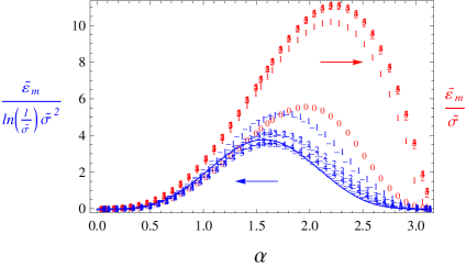
Figure 5: (Color online) Numerical result of the dimensionless membrane elastic energy $\widetilde{\varepsilon}_{m}=\varepsilon_{m}/\kappa$ as a function of $\alpha$. The eleven sets of data points are at $\widetilde{\sigma}=10^{-5},10^{-4},10^{-3},...,10^{5}$. They are labelled correspondingly as $-5,-4,-3,...5$. The left axis $\widetilde{\varepsilon}_{m}/\widetilde{\sigma}$ is for all $\widetilde{\sigma}\geq 1$ data points (red on line), while the right axis $\widetilde{\varepsilon}_{m}/\widetilde{\sigma}^{2}\ln(1/\widetilde{\sigma})$ is for all $\widetilde{\sigma}<1$ data points (blue on line), as indicated by the two arrows. The curve represents the analytical asymptotic solution (30) with an additional factor $1.3$ (blue on line), fitting the data points for $\widetilde{\sigma}\ll 1$.

The direct numerical result of $\varepsilon_{m}$ is plotted in Fig. 5, where for convenience we used the dimensionless elastic energy $\widetilde{\varepsilon}_{m}=\varepsilon_{m}/\kappa$. The first important thing to notice is that the elastic energy profile always takes a “sand dune” shape, where two minimums, zeros, are achieved at $\alpha\rightarrow 0,\pi$, and a maximum shows up in the middle of $\alpha$. Physically, this energy profile comes from the need of matching boundary conditions at the edge of the capsid and at infinity. The membrane deformed by the capsid edge at one end has to become flat far away from the capsid. At $\alpha\rightarrow 0$ and $\alpha\rightarrow\pi$, the membrane is not deformed at all, and the elastic energy is zero nec . While for $\alpha$ close to $\pi/2$, the membrane is almost vertical at the edge of the capsid, and a large amount of elastic energy is needed to bend it flat.

Secondly, we see clearly two kinds of asymptotic behaviors of $\varepsilon_{m}$ depending on the parameter $\widetilde{\sigma}=R/r_{s}$. In the stiff membrane regime, $\widetilde{\sigma}\gg 1$, the energy is proportional to $\widetilde{\sigma}$ as shown by the collapse of the data points to a single curve with $\widetilde{\sigma}$ varying from $10^{2}$ to $10^{5}$. The maximum of the energy is achieved at $\alpha_{m}\simeq 0.7\pi$. $\alpha_{m}$ is a nonlinear result and can not be calculated analytically. However, the proportionality of $\varepsilon_{m}$ to $\widetilde{\sigma}$ is a small deformation result as shown in Eq. (31). In the soft membrane regime, $\widetilde{\sigma}\ll 1$, the energy is proportional to $\widetilde{\sigma}^{2}\ln(1/\widetilde{\sigma})$, shown again by the collapse of the data points with $\widetilde{\sigma}$ varying from $10^{-2}$ to $10^{-5}$. Here the collapse is not as pronouncing as in the other regime mostly due to the larger numerical error in dealing with smaller $\widetilde{\varepsilon}_{m}$. The absolute value of $\widetilde{\varepsilon}_{m}$ in this regime is smaller at least in four order of magnitude than in the other regime. The maximum of the energy here is arrived at $\alpha_{m}=\pi/2$ and the curve becomes symmetric about $\alpha_{m}$. These features agree with our small $\widetilde{\sigma}$ solution originating from the catenoid solution. In fact, Eq. (30) fits the numerical data reasonably well, with an additional factor $1.3$.

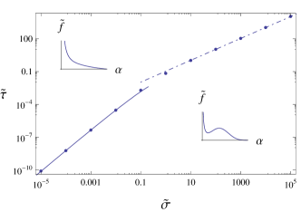
Figure 6: An effective “phase diagram” in the plane of two dimensionless parameters, $\widetilde{\sigma}=R/r_{s}$ and $\widetilde{\tau}=R\tau/\kappa$. In the upper-left part, the free energy density decreases monotonically with $\alpha$, while in the lower-right part, it has a local minimum, as shown in the insets. The numerical data points mark the “phase boundary” at which the local minimum appears. The dotdashed line and the solid lines fit the data points using $\widetilde{\tau}=0.11\widetilde{\sigma}$ and $\widetilde{\tau}=0.065\widetilde{\sigma}^{2}\ln(1/\widetilde{\sigma})$ respectively.

The scaling of $\varepsilon_{m}$ with $\widetilde{\sigma}$ suggests a simple way to do the numerical calculation to the free energy density. When $\widetilde{\sigma}\gg 1$,

$$\widetilde{f}=\widetilde{\varepsilon}_{c}+\widetilde{\varepsilon}_{m}=2\pi\cot\frac{\alpha}{2}\widetilde{\tau}+g_{1}(\alpha)\widetilde{\sigma}$$

$$=\widetilde{\sigma}\left[2\pi\cot\frac{\alpha}{2}\frac{\widetilde{\tau}}{\widetilde{\sigma}}+g_{1}(\alpha)\right],$$ (42)

where $\widetilde{\varepsilon}_{c}=\varepsilon_{c}/\kappa$ and $g_{1}(\alpha)$ is some function given by the numerical computation. According to the last equality, up to an overall constant $\widetilde{\sigma}$, $\widetilde{f}$ is completely determined by only one parameter $\widetilde{\tau}/\widetilde{\sigma}$. Similarly, when $\widetilde{\sigma}\ll 1$,

$$\widetilde{f}=\widetilde{\sigma}^{2}\ln\frac{1}{\widetilde{\sigma}}\left[2\pi\cot\frac{\alpha}{2}\frac{\widetilde{\tau}}{\widetilde{\sigma}^{2}\ln(1/\widetilde{\sigma})}+g_{2}(\alpha)\right],$$ (43)

where $g_{2}(\alpha)$ is again given by numerical computation, although we know it from our analytical result Eq. (LABEL:eq:fcat). In this regime, $\widetilde{f}$ is determined by one parameter $\widetilde{\tau}/\widetilde{\sigma}^{2}\ln(1/\widetilde{\sigma})$. Below in studying the local minimum of $\widetilde{f}$, we therefore consider a single parameter dependence.

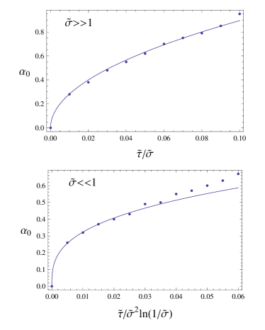
Figure 7: The capsid size $\alpha_{0}$ as a free energy local minimum is shown as a function of $\widetilde{\tau}/\widetilde{\sigma}$ and $\widetilde{\tau}/\widetilde{\sigma}^{2}\ln(1/\widetilde{\sigma})$ at two limits of $\widetilde{\sigma}$. The dots are numerical results taken at $\widetilde{\sigma}=10^{2},10^{3},10^{4},10^{5}$ for the upper panel and $\widetilde{\sigma}=10^{-2},10^{-3},10^{-4},10^{-5}$ for the lower panel. The curves are analytical results of Eq. (40) at $\widetilde{\sigma}\gg 1$ and Eq. (37) at $\widetilde{\sigma}\ll 1$ with additional numerical factors of 2 and $1.5$ respectively. The range of $\widetilde{\tau}$ plotted corresponds to the lower-right “phase” in the “phase diagram” of Fig. 6.

For all $\widetilde{\sigma}$ and $\widetilde{\tau}$, we get two different types of free energy density profiles as shown in Fig. 3, consistent with the analytical result for small $\widetilde{\sigma}$. The global minimum of the free energy density is always at $\alpha\rightarrow\pi$. Physically, the line tension energy prefers the shortest length of the capsid rim, which is zero for complete capsids ($\alpha\rightarrow\pi$). When $\widetilde{\tau}$ is very large, the line tension energy dominates, and the free energy density $\widetilde{f}$ decreases with $\alpha$ monotonically to zero, as shown in the left panel of Fig. 3. On the other hand, when $\widetilde{\tau}$ is small, due to the maximum of the membrane elastic energy $\varepsilon_{m}$, a local minimum at the capsid size, $\alpha_{0}$, shows up in the free energy density, as shown in the right panel of Fig. 3. It is useful to draw a “phase diagram” on the plane of $\widetilde{\sigma}$ and $\widetilde{\tau}$ as Fig. 6 to show this qualitative difference in the free energy density profile. The lower right region of Fig. 6 corresponds to value of the parameters ($\widetilde{\sigma}$, $\widetilde{\tau}$) where capsid budding can be kinetically trapped. The two lines fit the “phase boundary” at large and small $\widetilde{\sigma}$ with $\widetilde{\tau}=0.11\widetilde{\sigma}$ and $\widetilde{\tau}=0.065\widetilde{\sigma}^{2}\ln(1/\sigma)$ respectively. As one can see, there is a very good agreement between numberical results and our scaling formulas for $\widetilde{\sigma}$ in two asymptotic limits. According to the numerical fits, the threshold $\tau$ at which the local minimum in the free energy density shows up are

$$\tau_{c}=0.11\sqrt{\kappa\sigma}$$ (44)

when $\widetilde{\sigma}\gg 1$, and

$$\tau_{c}=0.065R\sigma\ln\frac{1}{R\sqrt{\sigma/\kappa}}$$ (45)

when $\widetilde{\sigma}\ll 1$. The later formula agrees with our analytical result Eq. (35) with a numerical factor 3 difference.

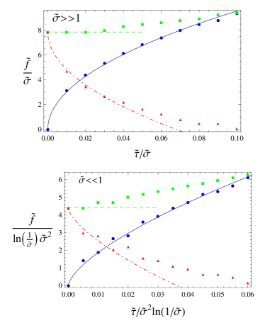
Figure 8: (Color online). The local minimum $\widetilde{f}_{0}$, maximum $\widetilde{f}_{m}$, and barrier $\widetilde{f}_{m}-\widetilde{f}_{0}$ of the free energy density. The values of $\widetilde{\sigma}$ and $\widetilde{\tau}$ plotted are the same as in Fig. 7. The circles (blue online) are the numerical result of $\widetilde{f}_{0}$, fitted by the solid lines (blue online) using Eq. (41) at $\sigma\gg 1$ and Eq. (38) at $\sigma\ll 1$ with additional numerical factor $1.7$ and $3.2$ respectively. The squares (green online) are the numerical result of $\widetilde{f}_{m}$, marked by the dashed lines (green online) at their zero $\widetilde{\tau}$ values. The triangles (red online) are numerical result of the barriers, $\widetilde{f}_{m}-\widetilde{f}_{0}$, fitted by the dotdashed lines (red online) using Eqs. (46) and (47).

The possible local minimum in $\widetilde{f}$ (the right panel in Fig. 3) suggests that budding may be trapped kinetically at the capsid size $\alpha_{0}$. Numerical and analytical results of $\alpha_{0}$ are shown in Fig 7. The analytical curves are drawn using Eq. (40) at $\widetilde{\sigma}\gg 1$ and Eq. (37) at $\widetilde{\sigma}\ll 1$, with additional numerical factors of 2 and $1.5$ respectively. There is a large deviation between analytical and numerical results at large $\widetilde{\tau}$. This is the parameter regime where the linear approximation is no longer valid.

The kinetic trapping becomes significant if the barrier in the free energy density is large. In Fig. 8, numerical and analytical results about this barrier are plotted. For the local minimum $\widetilde{f}_{0}$, up to a order one numerical factor ($1.7$ and $3.2$), our analytical expressions Eq. (41) at $\sigma\gg 1$ and Eq. (38) at $\sigma\ll 1$ remains reasonable approximation. We can not estimate the maximum $\widetilde{f}_{m}$, which is in the nonlinear regime. However, in the most important regime of small $\widetilde{\tau}$ and large barrier, Fig. 8 shows that the main contribution to $\widetilde{f}_{m}$ comes from the membrane elastic energy $\varepsilon_{m}$ (the value of $\widetilde{f}_{m}$ at $\widetilde{\tau}=0$). In this regime, the additional contribution to $\widetilde{f}_{m}$ from the line tension energy $\varepsilon_{c}$ is negligible and $\widetilde{f}_{m}$ is almost a constant. Combining the numerical result of $\widetilde{f}_{m}$ and the analytical result of $\widetilde{f}_{0}$ with proper numerical factors, we get the asymptotic formulas for the barrier at $\widetilde{\tau}\ll 1$,

$$\widetilde{f}_{m}-\widetilde{f}_{0} \simeq 7.8\widetilde{\sigma}-6.8\pi\sqrt{2\widetilde{\sigma}\widetilde{\tau}}$$ (46)

$$= 7.8R\sqrt{\frac{\sigma}{\kappa}}-6.8\pi R\sqrt[4]{\frac{4\sigma\tau^{2}}{\kappa^{3}}},\ \ (\widetilde{\sigma}\gg 1).$$

$$\widetilde{f}_{m}-\widetilde{f}_{0} \simeq 4.4\widetilde{\sigma}^{2}\ln(1/\widetilde{\sigma})-12.8\pi\sqrt[3]{\widetilde{\tau}^{2}\widetilde{\sigma}^{2}\ln(1/\widetilde{\sigma})}$$ (47)

$$= 4.4R^{2}\frac{\sigma}{\kappa}\ln\frac{\sqrt{\kappa/\sigma}}{R}-12.8\pi\frac{R}{\kappa}\sqrt[3]{\tau^{2}\sigma\ln\frac{\sqrt{\kappa/\sigma}}{R}},$$

$$(\widetilde{\sigma}\ll 1).$$

The largest barriers are achieved at $\widetilde{\tau}=0$ or $\widetilde{f}_{0}=0$.

VI kinetics of budding and partial budding

As discussed in the previous sections, with a finite Gag-Gag attraction, budding always proceeds to completion thermodynamically. However, when this attraction is weak, or $\tau$ is small, a metastable state of partial budding appears at a smaller capsid size $\alpha_{0}$ (see Fig. 3). It is therefore possible that the budding process is kinetically trapped at $\alpha_{0}$. In this section, we discuss this kinetic effect and make connections of our theory to experiments.

Let us first estimate the values of parameters. A normal plasma membrane has $\kappa\simeq 20-40\mathrm{k_{B}T}$ and $\sigma\simeq 0.5-2\mathrm{pN}/\mathrm{nm}=0.12-0.48\mathrm{k_{B}T}/\mathrm{nm}^{2}$ Morris and Homann (2001). On the other hand, typical HIV have $R\simeq 60-80\mathrm{nm}$ Coffin et al. (1997). Consequently, $\widetilde{\sigma}=R\sqrt{\sigma/\kappa}\simeq 10$ and only the stiff membrane regime with $\widetilde{\sigma}\gg 1$ is relevant for HIV. Actually in the opposite regime of $\widetilde{\sigma}\ll 1$, one can show that the typical energy scale $\varepsilon_{m}\sim\kappa\widetilde{\sigma}^{2}\ln(1/\widetilde{\sigma})$ is comparable to $\mathrm{k_{B}T}$ and thus not important in the room temperature. In this section, we therefore focus on the stiff membrane regime only.

In order to see if budding can be kinetically trapped at the local minimum $\alpha_{0}$ (see Fig. 3), we have to study the budding kinetics and calculate the kinetic barrier. For this purpose, let us employ the standard kinetic picture of the first order phase transition Lifshitz and Pitaevskii (1997); Nguyen and Shklovskii (2002), corresponding to the transition from a free-Gags phase to an aggregated Gags phase where Gags self-assemble into complete viral capsids. At the initial stage of aggregation, the concentration of free Gags is large, Gags coagulate to form dimers. Dimers coagulate with free Gags or other dimers to form larger Gag clusters (small capsids). This initial coagulation or nucleation is a fast process and is not a rate limiting step in retroviral budding. Soon free Gags are significantly depleted, and the main kinetic pathway for growth of capsids is for them to diffuse and merge with each other. We will be concern with this later stage of coagulation. For simplicity, we work with the dominant capsid size, $\alpha(t)$ [with concentration $n(t)$], assuming these typical capsids carry all the mass of membrane-bound Gag proteins.

Let us start with the case when $\alpha(t)$ is still small so that the energy barrier for merging of capsids is smaller than $\mathrm{k_{B}T}$. This is the regime of the well known diffusion limited aggregation Evans and Wennerström (1999). The rate of the capsid area $A(\alpha,t)$ incretion is proportional to the probability that two capsids diffuse and merge with each other. The kinetic rate equation reads

$$\frac{dA(\alpha,t)}{dt}=2\pi R\sin\alpha(t)A(t)D\nabla n(t)|_{R\sin\alpha},$$ (48)

where $D\simeq k_{B}T/\eta R\sin\alpha(t)$ is the lateral diffusion constant of a capsid on the membrane and $\nabla n(t)|_{R\sin\alpha}$ is the gradient of the concentration $n(t)$ on the edge of the capsid. This gradient can be estimated assuming a steady state in the diffusion and taking the adsorbing boundary condition at the edge of the capsid and a given capsid concentration [Eq. (3)] far away from the capsid. Solving the diffusion equation with these boundary conditions, we find

$$\nabla n(t)|_{R\sin\alpha}=\frac{c_{G}A(\alpha_{G})}{A(\alpha)R\sin\alpha}.$$ (49)

Substituting these relations and Eq. (4) into Eq. (48), we get

$$\frac{\alpha(t)}{2}-\frac{\sin 2\alpha(t)}{4}=\frac{t}{\tau_{diff}}+\frac{\alpha_{G}}{2}-\frac{\sin 2\alpha_{G}}{4}.$$ (50)

where

$$\tau_{diff}=\eta R^{3}/Tc_{G}A(\alpha_{G})$$ (51)

is the time scale of diffusion proportional to the viscosity $\eta$ of the membrane. In the small $\alpha$ regime corresponding to a small kinetic barrier, this equation can be written as

$$\alpha(t)=(3t/\tau_{diff}+\alpha_{G}^{3})^{1/3},$$ (52)

which is a slow function of time.

The regime of diffusion limited growth stops when the kinetic barrier between approaching partial capsid is much larger than $k_{B}T$. At a later time, a different growth regime of Lifshitz-Slezov (LS) comes into play Lifshitz and Pitaevskii (1997). In this mechanism, the growth is no longer due to collision and merging of partially budded capsids. Instead, smaller capsids shrink and release individual Gags. These Gag are absorbed into larger capsids, leading to their growth. This process of releasing and adsorbing of individual Gags (the so-called coalescence) has much smaller kinetic barrier than the barrier to capsid merging in this later stage. The growth of capsid size in LS regime is the same as that of diffusion limited growth Lifshitz and Pitaevskii (1997). However, the rate constant $\tau_{LS}$ depends exponentially on the activation energy to release individual Gag proteins from a capsid

$$\tau_{LS}\propto\exp(-|\epsilon|/k_{B}T)$$ (53)

where $\epsilon$ is the binding energy of Gag in a capsid, which itself is also a function of the Gag-Gag interaction.

The kinetic picture described above is good when $\tau>\tau_{c}$ and the free energy density decreases monotonically with increasing $\alpha$ (the left panel of Fig. 3). However, when $\tau<\tau_{c}$ and a local minimum $\alpha_{0}$ appears in the free energy density (the right panel of Fig. 3), the above picture must be modified. For the cluster growth, either in the diffusion-limited regime or in the LS regime, the growth of the cluster size always reduces the free energy of the system. On the other hand, for the capsid growth of retroviral budding, after the capsid size reaches $\alpha_{0}$, the system free energy increases when the capsids grow further. For $\alpha>\alpha_{0}$, the growth of capsids is determined by the ability to tunnel through the kinetic barrier related to $f_{m}-f_{0}$ (see Fig. 3). The detail analysis of the rate of capsid growth for $\alpha>\alpha_{0}$ is a very interesting problem by itself, requiring understanding of membrane energetics when a partially budded capsid absorbs other capsids or many individual Gags to increase its size from $\alpha_{0}$ to $\alpha_{m}$. These calculations are beyond the scope of this paper and we will leave the detail treament of capsid growth in this case to a future study. Nevertheless, one can expect the rate of such process to inversely proportional to the exponential of the energy barrier

$$\tau_{tunnel}\propto\exp[-(f_{m}-f_{0})/nk_{B}T],$$ (54)

where $(f_{m}-f_{0})/n$ is the energy barrier of a membrane cell with a single capsid in it. According to Eqs. (46) (see also the upper panel of Fig. 8), the maximum energy barrier is achieved at $f_{0}=0$ or $\widetilde{\tau}=0$. Using Eqs. (3) and (LABEL:eq:fcat), it can be written as

$$E_{m}=\frac{f_{m}}{n}=\kappa(1-\cos\alpha_{m})\widetilde{f}_{m},$$ (55)

where $\widetilde{f}_{m}$ is given by Eqs. (46), and $\alpha_{m}$ is the corresponding capsid size. A more useful expression of $E_{m}$ can be got if one recognizes that $E_{m}$ is nothing but the maximum of $\varepsilon_{m}$ shown in Fig. 5. Using the numerical result of that figure, we get

$$E_{m}=11.5\kappa\widetilde{\sigma}=11.5R\sqrt{\kappa\sigma}.$$ (56)

Clearly, $E_{m}\gg\mathrm{k_{B}T}$ for $\widetilde{\sigma}>1$. For example, for $R=70\texttt{nm}$, $\sigma=0.24\mathrm{k_{B}T/nm^{2}}$ and $\kappa=20\mathrm{k_{B}T}$, we get $E_{m}=1765\mathrm{k_{B}T}$. The true energy barrier is smaller than $E_{m}$ since $\widetilde{\tau}>0$. In the regime of small $\widetilde{\tau}$, according to Eq. (46), it is

$$E \simeq \kappa(1-\cos\alpha_{m})(\widetilde{f}_{m}-\widetilde{f}_{0})$$ (57)

$$= E_{m}\left(1-3.9\sqrt{\frac{\widetilde{\tau}}{\widetilde{\sigma}}}\right)=E_{m}\left(1-3.9\sqrt[4]{\frac{\tau^{2}}{\kappa\sigma}}\right).$$

In experiments, if one treats $\kappa$ and $\sigma$ as constants then according to Eq. (56) the larger the retrovirus size $R$, the bigger the kinetic barrier. On the other hand, the line tension $\tau$ is directly proportional to the strength of the Gag-Gag attraction and is experimentally adjustable through mutation of the late domain on the Gag protein, binding of other molecules to Gags or changing the pH, salinity of water solution near the membrane Morita and Sundquist (2004); Campbell et al. (2001). As we know, the closest approach distance between two Gag proteins is about $10\mathrm{nm}$ Coffin et al. (1997). If Gags are densely packed on the capsid, this gives $\tau\simeq 0.5\mathrm{k_{B}T}/\mathrm{nm}\simeq 2\mathrm{pN}$ for normal retroviral capsids. Theoretically, in order to have a local minimum in the free energy density and trap retrovirus budding kinetically, we must have $\tau<\tau_{c}$ (see Fig. 3). For a normal cell membrane with $\kappa=20\mathrm{k_{B}T}$ and $\sigma=0.24\mathrm{k_{B}T}/\mathrm{nm}^{2}$, using Eq. (44), $\tau_{c}\simeq 0.24\mathrm{k_{B}T}/\mathrm{nm}=1\mathrm{pN}$. Therefore for normal capsids, $\tau>\tau_{c}$, and budding easily proceeds to completion (see the left panel of Fig. 3). One the other hand, $\tau$ is bigger than $\tau_{c}$ only by a factor of 2. Therefore HIV budding can be fairly easily trapped at a partially budded state with capsid size $\alpha_{0}$ by reducing the Gag-Gag interaction strength such as mutation of a single domain on the Gag protein. The kinetic barrier $E$ appeared at $\alpha=\alpha_{0}$ can be much larger than $\mathrm{k_{B}T}$, and the time scale for capsid growth beyond $\alpha_{0}$, $\tau_{tunnel}$, is exponentially large. Qualitatively, this trend is consistent with experiments on mutation of the late domain of Gag proteins Morita and Sundquist (2004); Demirov and Freed (2004). Numerically, we know that $\alpha_{0}<0.9\simeq 0.3\pi$ (see the upper panel of Fig. 7). It agrees with experiments reasonably well, although there are many additional factors that we neglected in our treatment such as local variation in membrane elasticity due to raft structures or the presence of other proteins in in-vivo assembly and budding. More controlled experiments are needed to to verify the dependence on the membrane rigidities and Gag-Gag attraction of $\alpha_{0}$ given by Eq. (40).

VII Conclusion

In this paper, we developed an elastic model of HIV (and retroviruses in general) budding and self-assembly on the elastic membrane. We studied the free energy profile of the system as a function of the capsid size $\alpha$. We showed that although always thermodynamically favorable, complete budding and assembly may not be achieved if the Gag-Gag attraction is weak. In practice, for normal biological conditions, the Gag-Gag attraction is strong enough and HIV budding and assembly always proceed to completion, as it should be. On the other hand, it is fairly easy to trap HIV budding to a partially budded state with capsid size $\alpha_{0}$ by reducing the Gag-Gag attraction. This can be done through the mutation of late domain on the Gag protein or binding of other molecules to Gag. In principle, the trapping is also possible by increasing the membrane rigidities, although this is not easy to do in vivo. Our theory agrees with reasonably well with experimental results. However, experiments with better controlled environments are needed to verify various aspect of the theory.

The most interesting point of our model is probably that it provides a unique self-assembly mechanism. Not like self-assembly of other viruses or colloids, HIV assemble and bud concurrently on the membrane. Therefore the membrane elastic energy plays an important role in the assembly process. For example, the kinetic barrier which traps the HIV budding essentially comes from the membrane elastic energy around the capsids. In fact, our model developed for HIV budding and assembly can be very well applied to other situations. For example, for a given concentration of membrane-bounded proteins with a fixed spontaneous curvature, this kind of budding and assembly phenomenon should also exist and can be explained using our model. In this situation, it may be easier to change the membrane properties and protein-protein attraction in vitro to verify our theory more quantitatively. Due to the interplay between the membrane elastic energy and the Gag-Gag attraction energy, the kinetics of retrovirus budding is an interesting problem by itself, as discussed in Sec. VI. We plan to address this question in more detail the near future.