Magnetic phases of one-dimensional lattices with 2 to 4 fermions per site

Abstract

We study the spectral and magnetic properties of one-dimensional lattices filled with 2 to 4 fermions (with spin 1/2) per lattice site. We use a generalized Hubbard model that takes account all interactions on a lattice site, and solve the many-particle problem by exact diagonalization. We find an intriguing magnetic phase diagram which includes ferromagnetism, spin-one Heisenberg antiferromagnetism, and orbital antiferromagnetism.

I introduction

Artificial lattices resemble periodic arrangements of quantum wells confining a small number of particles. Experimentally, both lateral and vertical lattice structures can be realized. Examples are arrays of quantum dots in semiconductor heterostructures lee2001 ; schmidbauer2006 ; kohmoto2002 confining the conduction electrons, or optical lattices – stable periodic arrays of potentials created by standing waves of laser light eurphysnews ; jaksch2005 . Varying the intensity of the laser light, one can change the depths of the single traps, i.e. the single sites. In such egg-box like potentials, experimentalists can confine ultra-cold atoms, of bosonic or fermionic character greiner2002 ; han2000 ; kerman2000 ; modugno2003 ; rom2006 ; chin2006 , achieving particle numbers on the sites that are even less than three. The strengths and even the sign of the interactions between the atoms can be tuned by Feshbach resonances feshbach1958 ; inouye1998 ; courteille1998 ; roberts1998 ; duine2004 ; theis2004 .

The basic difference between artificial lattices and normal lattices (such as the crystal structure of solids) is, that in artificial lattices the particles confined in the lattice do not play any role for determining the intrinsic lattice structure. A possible degeneracy of the many-particle states can then not be removed by lattice distortion. Instead, it may lead to internal symmetry breaking and, for example, to spontaneous magnetism and superconductivity. Recent experiments have inspired much theoretical work on artificial lattices, both with cold atoms gu2007 ; xianlong2007 ; massel2005 ; koponen2006 ; koponen2007 and quantum dots chen1997 ; taut2000 .

Mean-field calculations based on the spin-density functional theory predict that Hund’s first rule determines the total spin of an isolated, individual lattice site koskinen1997 ; reimann2002 . The magnetism of the lattice as a whole then depends on the total spin of the individual lattice sites, on the lattice structure and on the coupling between the siteskoskinen2003 ; karkkainen2007 ; karkkainen2007a ; karkkainen2007b . A simple tight-binding model with a few parameters can account for most of the these findingskoskinen2003b . Related results have been obtained for quantum dot molecules using the density functional methodkolehmainen2000 .

The eigenstates of single quantum dots with a few electrons can be calculated “exactly” (i.e. to a high degree of convergence with respect to the necessary restrictions in Hilbert space) by diagonalizing the many-body Hamiltonian (for a review see Ref.reimann2002 ). Methods beyond the mean-field approximation have also been applied to quantum dot moleculesyannouleas1999 ; bayer2001 ; harju2002 ; mireles2006 ; scheibner2007 ; zhang2007 .

For a lattice with strongly correlated particles the generic model is the Hubbard model, which has been amply studied in the case of one state per lattice site (for reviews seevoit1994 ; kolomeisky1996 ). From an experimental viewpoint, it has been argued that the Hubbard approach is ideal for describing contact-interacting atoms in an optical lattice jaksch98 ; greiner02 ; stoferle2004 ; xu2005 ; jaksch2005 . The one-dimensional Hubbard model is exactly solvable using the Bethe ansatzlieb1968 . The magnetism of finite moleculespastor1994 ; lopezurias1999 and quantum ringsviefers2004 have also been studied in the simple Hubbard model.

The purpose of this paper is to study the magnetism of an artificial one-dimensional (1D) lattice in the case where the lattice site is filled on average with 2 to 4 fermions, which can be electrons in a quantum dot lattice or fermionic atoms in an optical lattice. We call the electrons or atoms generally as particles. We assume the confining potential in each lattice site to be quasi-two-dimensional and nearly harmonic at the bottom. In this case the $1s$-level of each lattice site is filled, and the degenerate $1p$ level is partially filled. We use a generalization of the Hubbard model to describe the interactions: The particles interact only within a lattice site. We solve the Hubbard Hamiltonian by exact diagonalization for a finite length of the lattice using periodic boundary conditions. The results show many different magnetic structures which are analyzed through their relations to the Heisenberg model and the simple single-state Hubbard model.

II Theoretical models

II.1 1D lattice with $p$-orbitals

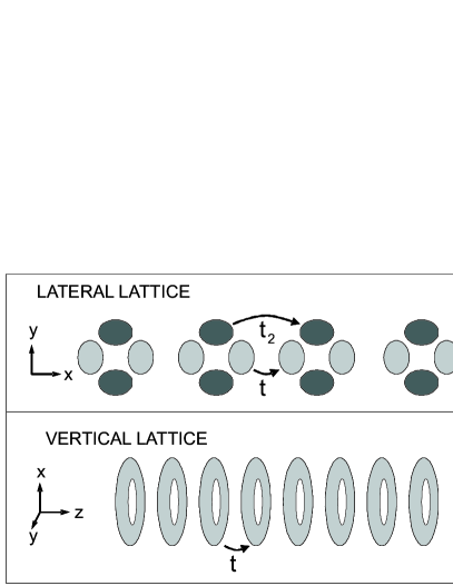
Figure 1: Schematic pictures of 1D lattices considered. Each lattice site has $p_{x}$ and $p_{y}$ orbitals. In the lateral case these are shown as light and dark-gray densities. Here, the hopping probabilities $t$ and $t_{2}$ between neighboring lattice sites are different for $p_{x}$ and $p_{y}$ orbitals. In the vertical case it is natural to use states with ’rotating orbitals’ $p_{+1}$ and $p_{-1}$ with circularly symmetric densities. In this case there is only one hopping probability $t$.

We consider an artificial lattice where the confining potential at each lattice site is nearly harmonic and quasi-two-dimensional so that the single-particle level structure in each lattice site is $1s$, $1p$, $2s1d$ etc. We assume that in all cases the $1s$-state is filled completely, and the doubly degenerate $1p$-level is partially filled. Furthermore, we assume that the shells are well separated in energy, so that we can neglect the mixing of the $1p$ shell with the $1s$ or $2s1d$ shells. This leads to a generalized Hubbard model which has in each lattice site only two orbitals which we call either $p_{x}$ and $p_{y}$ or $p_{-1}$ and $p_{+1}$, respectively. The latter notation refers to orbitals with angular momentum quantum numbers $-1$ and $+1$ (clockwise or counterclockwise rotation of the $p$-state).

The two kinds of 1D lattices considered are schematically shown in Fig. 1. In the case of semiconductor quantum dots, these are often called lateral and vertical structures. In the lateral lattice the hoppings between neighboring $p_{x}$ and $p_{y}$ states are different and denoted by $t$ and $t_{2}$, where $t_{2}<t$. For the vertical lattice, it is natural to use the angular momentum states $p_{-1}$ and $p_{+1}$. In that case there is only one hopping parameter $t$ (or equivalently $t_{2}=t$). Note that for the single-particle wave functions we have $\psi_{+1}=(\psi_{p_{x}}+i\psi_{p_{y}})/\sqrt{2}$ and $\psi_{-1}=(\psi_{p_{x}}-i\psi_{p_{y}})/\sqrt{2}$.

II.2 Hubbard model

We assume a generalized Hubbard model Hamiltonian

$$\hat{H}=\hat{J}+\hat{U},$$ (1)

where the first term represents inter-site hoppings between neighboring lattice sites and the second term intra-site two-body interactions.

Hoppings preserve spin, and are equal for spin-up and spin-down particles. Thus, $\hat{J}$ separates into two symmetric spin parts: $\hat{J}=\sum_{\sigma=\uparrow,\downarrow}\hat{J}_{\sigma}$. For our one-dimensional lattice with $p$-orbitals

$$\hat{J}_{\sigma}=-\sum_{n}\sum_{jj^{\prime}}J_{jj^{\prime}}\left(c^{\dagger}_{nj\sigma}c_{n+1j^{\prime}\sigma}+h.c.\right),$$ (2)

where $n$ is the lattice site index, and $j$ and $j^{\prime}$ denote the $p$-orbital in question. (In the simple Hubbard model, there would be only one space state per site, and the $j$-indices not needed).

Some of the hopping integrals $J_{jj^{\prime}}$ are zero due to symmetry. The non-zero integrals are treated as essentially free model parameters, $t$ and $t_{2}$. Thus, we have

$$\begin{array}[]{lll}j&j^{\prime}&J_{jj^{\prime}}\\ \hline\cr p_{x}&p_{x}&t\\ p_{y}&p_{y}&t_{2}\\ p_{x}&p_{y}&0\\ \hline\cr\end{array}\hskip 28.45274pt\begin{array}[]{lll}j&j^{\prime}&J_{jj^{\prime}}\\ \hline\cr p_{-1}&p_{-1}&t\\ p_{+1}&p_{+1}&t\\ p_{-1}&p_{+1}&0\\ \hline\cr\end{array}$$

for the lateral and vertical lattice, respectively. (Note, that in the case $t_{2}=t$, the lateral model actually is identical to the vertical model, irrespective of the different $p$-orbit basis used).

We approximate the two-body interactions in the spirit of the tight-binding model: The particles only interact when they are at the same lattice site. Thus, $\hat{U}$ separates in the symmetric parts representing interactions on each site $n$: $\hat{U}=\sum_{n}\hat{U}_{n}$. Within a site, full (spin-indpendent) two-body interaction is allowed, which yields

$$\hat{U}_{n}={1\over 2}\sum_{\stackrel{{\scriptstyle j_{1}j_{2}j_{3}j_{4}}}{{\sigma\sigma^{\prime}}}}U_{j_{1}j_{2}j_{3}j_{4}}c_{nj_{1}\sigma}^{\dagger}c_{nj_{2}\sigma^{\prime}}^{\dagger}c_{nj_{4}\sigma^{\prime}}c_{nj_{3}\sigma}$$ (3)

where $U_{j_{1}j_{2}j_{3}j_{4}}$ are the direct space matrix elements of on-site interaction, depending on the interaction itself and the $j$-orbits in question, i.e. the eigenstates of the confining potential.

For contact interactions, the ratios of the different matrix elements are independent of the confining potential, as long as it has circular symmetry. For the non-zero matrix elements (together with those obtained by allowed $j$-index permutations), we obtain

$$\begin{array}[]{ccccc}j_{1}&j_{2}&j_{3}&j_{4}&U_{j_{1}j_{2}j_{3}j_{4}}\\ \hline\cr p_{x}&p_{x}&p_{x}&p_{x}&3U\\ p_{x}&p_{x}&p_{y}&p_{y}&U\\ p_{x}&p_{y}&p_{x}&p_{y}&U\\ p_{x}&p_{y}&p_{y}&p_{x}&U\\ p_{y}&p_{y}&p_{y}&p_{y}&3U\\ \hline\cr p_{-1}&p_{-1}&p_{-1}&p_{-1}&2U\\ p_{-1}&p_{+1}&p_{-1}&p_{+1}&2U\\ p_{-1}&p_{+1}&p_{+1}&p_{-1}&2U-\Delta\\ p_{+1}&p_{+1}&p_{+1}&p_{+1}&2U\\ \hline\cr\end{array}$$

where $U$ is the only parameter describing the strength of the interaction. All together, we thus have three parameters $t$, $t_{2}$ and $U$. One of them can be fixed to set the energy scale. We choose this to be $t$ and represent the results for $t=1$ (all energies are given in units of $t$). In some cases with vertical lattices we also consider an interaction of finite width. This can be mimicked by decreasing one of the matrix elements by a small amount $\Delta$, as indicated in the above table. For contact interactions, $\Delta=0$.

We solve the Hamiltonian for a lattice with $L$ lattice sites using periodic boundary conditions ($\hat{J}$ connects also the last and the first site). The Lanczos method is used to find the low-energy eigenvalues and eigenvectors of the Hamiltonian matrix. We take advantage of the periodicity of the lattice and solve the eigenvalues separately for each Bloch $k$-value. In practice this means that, instead of using “site-states” $\mid nj\sigma\rangle$ as a single-particle basis to span the Fock space, one uses Bloch states of the tight-binding model (eigenstates of $\hat{J}$). In this study, the hopping does not mix the $p_{x}$ and $p_{y}$ orbitals in the lateral case, nor $p_{-1}$ and $p_{+1}$ orbitals in the vertical case. We then have separate, simple bands with energy eigenvalues

$$\epsilon_{t}(k)=-2t\cos\left(\frac{2\pi k}{L}\right),$$ (4)

where $k$ takes integer values $0,~{}1,~{}\cdots,L-1$. Note that in the lateral case, the $p_{x}$ and $p_{y}$ bands have different widths for $t$ and $t_{2}$, respectively. In the vertical case, the widths are always the same.

We do not take advantage of the fact that the Hamiltonian does not depend on spin, but diagonalize the system for $S_{z}=0$ and only afterwards determine the total spin $S$ for each many-particle state. The total number of particles is denoted by $N$ and the numbers of spin-up particles and spin-down particles by $N_{\uparrow}$ and $N_{\downarrow}$. We note that because of the spin degree of freedom, the maximum number of particles in a lattice with length $L$, is $N_{\text{max}}=4L$. The filling fraction by $\nu=N/L$ gets values from 0 to 4. In this study we consider only the region $\nu=0\cdots 2$. Due to the symmetry of the Hamiltonian the region $\nu=2\cdots 4$ will have similar properties.

As discussed earlier, we assume that the hopping can occur only between the nearest neighbours. It should be noted, however, that the interaction part of the Hamiltonian allows intra-site hopping, via scattering from one single-particle state to another inside any lattice site. This becomes important especially in the case where $t_{2}=0$, where the hopping only occurs through the $p_{x}$ states.

II.3 Heisenberg model

It is well-known that the simple Hubbard model in the limit of large $U/t$ approaches the antiferromagnetic Heisenberg model. In this case, the low-lying eigenstates are characterized by one spin $1/2$ particle on each site. In a similar way, in some limiting cases, our results with $p$-orbitals approach those of the Heisenberg model with $S=1$ (two particles on each site with aligned spins), or with $S=1/2$ (polarized system with one fermion on each site, with the $p$-orbitals playing the role of the spin components). The effective Hamiltonian is then

$$\hat{H}_{\rm eff}=J_{\rm eff}\sum{\bf S}_{n}\cdot{\bf S}_{n+1}+\text{constant},$$ (5)

where $J_{\rm eff}$ is the effective exchange interaction and ${\bf S}_{n}$ the spin operator for site $n$. We compare the Heisenberg and Hubbard model for the case of four sites, $L=4$, where the spectrum of the antiferromagnetic Heisenberg model is exactly solvableashcroft1976 ; viefers2004 .

III Results

III.1 A single lattice site with two particles

A single site with two particles obeys Hund’s first rule to maximize the spin. The energy difference between the lowest $S=0$ and $S=1$ states is the ’exchange splitting’ and equals $\Delta E=E_{S=0}-E_{S=1}=2U$. In the case of a finite-range interaction the exchange splitting is $2U-\Delta$. Table LABEL:singleatom gives the energy spectrum of a single lattice site. We will see below that in the limit of large $U$ the half-filled system ($\nu=N/L=2$) becomes a Heisenberg antiferromagnet with $S=1$.

Table 1: Energy levels and corresponding total spin of a single lattice site with two particles.

State No	$E$	$S$
1	$\Delta$	1
2	$2U$	0
3	$2U$	0
4	$4U-\Delta$	0

III.2 Half-filled vertical lattice: $N=2L$

Figure 2: Low-energy levels ($E\ll U$) for $L=4$ and $N=8$ calculated for different values of $U$. The numbers next to the levels denote the total spin $S$ of the many-particle state. The wave vector $k$ has values 0, 1, and 2. The symbols plus, square, star, circle and dot correspond to $U$ values 2, 2.5, 5, 10, and 50, respectively. The energy levels for $U=50$ agree with those of the $S=1$ Heisenberg model with 0.01 % accuracy.

In the half-filled case there is one particle per orbital. When $U$ is large, each lattice site will have spin $S=1$ due to the large exchange splitting. The only way to allow particles to hop from one site to the neighboring one is to orient the total spins of neighboring sites opposite, i.e. with antiferromagnetic order. For ferromagnetic order, the hopping would be prohibited by the Pauli exclusion principle. In this case the total energy of the system would be zero (assuming $\Delta=0$). For antiferromagnetic order the allowed hopping can reduce the energy to a slightly negative value.

We will first study the case of vertical lattice ($t_{2}=t$). Figure 2 shows the low-energy energy levels for four lattice sites and eight particles ($L=4$, $N=8$), calculated for different values of $U$. All the levels with energy $E\stackrel{{\scriptstyle<}}{{\sim}}U$ are shown. For the largest value $U=50$ the spectrum agrees with that of the Heisenberg model ($J_{\rm eff}=2/U$) with 0.01 % accuracy. The Heisenberg model for four sites is an exacly solvable textbook problemashcroft1976 ; viefers2004 . It is interesting to notice that even for $U=2$ the spectrum is qualitatively still the same. Only when $U\lesssim 1.5$ new states start to appear in the low-energy spectrum.

III.3 Vertical lattice polarized fermions: The noninteracting case

We will now consider polarized fermions (e.g. electrons or fermionic atoms with $N=N_{\uparrow}$). For contact interactions between the fermions, the problem becomes non-interacting since the Pauli exclusion principle forbids two fermions to be at the same state. The energy spectrum can then be constructed by filling particles to the Bloch states (Eq. (4)) which are solutions of the noninteracting Hamiltonian $\hat{J}$.

In this (trivial) case, it is important to note that $(i)$ each single-particle Bloch state is doubly degenerate due to the two states per site, and $(ii)$ only for particle numbers $N=4n+2$ the ground state is non-degenerate ($n$ is a non-negative integer). $(ii)$ implies that the ground state energy (of polarized fermions) as a function of $N$ has local minima for $N=2,~{}6,~{}10,\cdots$. We will see later that these special values form single domain ferromagnets when $N<2L$.

III.4 Orbital antiferromagnet of polarized fermions: Vertical lattice with $N=L$

Figure 3: Low-energy levels ($E\leq 0$) for polarized fermions with $L=4$ and $N=4$ calculated for different values of $\Delta$ for $U=50$. The numbers next to the levels denote the total spin of the corresponding state of the spin-1/2 Heisenberg model. The wave vector $k$ has values 0, 1, and 2. The symbols star, circle and dot correspond to $\Delta$ values 2, 10, and 50, respectively. The energy levels for $\Delta=50$ agrees with those of the $S=1/2$ Heisenberg model with 0.1 % accuracy.

Let us now consider polarized fermions with a finite range interaction and one fermion per lattice site ($N=N_{\uparrow}=L$). The finite range here means only that $\Delta>0$. However, the finite range does not lead to interaction of particles sitting at different lattice sites. Each site still has two $p$ states. The large $U$ limit in this case is an antiferromagnet where the ’magnetic moment’ in each lattice site is not the spin but the orbital angular momentum of the $p$ states, which can have the two values +1 or -1.

There are two reasons for this state to become the ground state. First, it costs energy (by $\Delta$) for two particles to occupy the same site. Thus, the particles prefer to be at different sites. Second, the particles can only hop to the neighboring site if they are at different orbital states. Although the particles prefer to be at different sites, a small amount of ’virtual’ hopping is necessary to reduce the energy.

Again, we compare the spectrum with the exact result of the Heisenberg model for four particles. In Fig. 3, all the low energy states are plotted for different $k$ values. For large $U$ and $\Delta$ the agreement between the Hubbard model and Heisenberg model becomes perfect with $J_{\rm eff}=1/\Delta$.

III.5 Vertical lattices with $N<2L$: Ferromagnetism

Next, we consider vertical lattices with contact interactions and large values of $U$ ($U\geq 10$). The results show that the ground states for $N=2,~{}6,$ and $10$ have maximum possible total spin, i.e. they are ferromagnetic. This is true for all values of $L>N/2$ where the computations could be performed (the matrix sizes increase very fast with $L$). The ferromagnetic ground state can be understood as follows. When $L\gg N/2$ the ferromagnetic state allows particles to move freely in the lattice, as even in cases where two particles are in the same lattice site, they do not interact. In other words, particles with the same spin can pass each other without any cost of energy. If the particles have opposite spin, however, they suffer repulsive interaction whenever they are at the same lattice site – even if they are at different $p$-states.

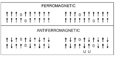
Figure 4: Motion of holes in the nearly half-filled case with large $U$ which prevents two opposite spins to be at the same lattice site. In the ferromagnetic case, the holes can move independently, while in the antiferromagnetic case they are bound together since their separation costs energy, as indicated by $U$.

Let us now consider what happens if we start from the antiferromagnetic $L=N/2$ state and increase $L$ by one. Also in this case the results show that, independent of the particle number (here, $2\leq N\leq 10$), the ground state is ferromagnetic. In the antiferromagnetic case with $L=N/2$ the lowest energy is proportional to $-1/U$, which for large $U$ is very small. The energy of the ferromagnetic case with $L=N/2$ is zero since there is no room for hopping (the single-particle bands are filled). If now one lattice site is added, the ferromagnetic energy becomes $-4t$. This is because there are now two freely moving holes in the system, as illustrated in Fig. 4. The situation is different if the system remains antiferromagnetic. Also in this case there are two holes, but now they are bound together, since their separation costs energy, as illustrated in Fig. 4. The total energy of the antiferromagnetic state will necessary be above the ferromagnetic energy $-4t$. Consequently, adding one lattice site to the antiferromagnetic $L=N/2$ case transforms it to a ferromagnetic state. Alternatively, we can start from the half-filled case and remove one particle. In the ferromagnetic case the hole is free and has an energy of $-2t$, while in the antiferromagnetic case the hole is localized and its energy is zero.

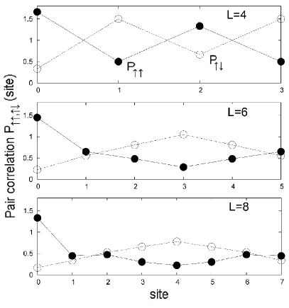
Figure 5: Pair-correlation of vertical lattices of different lengths $L=4,~{}6,~{}8$ with $N=8$ fermions. In each case the reference site is 0 where one particle with spin-up is fixed. The solid line with black dots shows the total up-up correlation and the dashed line with open circles the up-down correlation. The uppermost panel shows the antiferromagnetic ground state of $L=4$, the center panel and the lowest panel show the two domains of the ferromagnetic ground states of $L=6$ and $L=8$, respectively.

As mentioned above, the ferromagnetic ground state has total spin $S=N/2$ for $N=2,~{}6,~{}10,~{}\cdots$. However, the situation is more complicated for $N=4,~{}8,~{}12,~{}\cdots$. In these cases the total spin of the ground state is $S=0$ for all $L>N/2$. Nevertheless, we argue that also these cases are ferromagnetic, but now the ground state has a spin wave which rotates the spin once within the length $L$. Alternatively, we can apply the picture that the ferromagnetic ground state consists of two domains with opposite spin directions. The reason for this behavior is the fact that for these particle numbers the ferromagnetic state is degenerate and the spin wave (or domain formation) provides a way to remove the degeneracy and reduce the total energy.

Figure 5 shows the pair-correlation function of $N=8$ particles for $L=4$, 6, and 8. We fix one particle in a state, say $p_{+1}$ with spin-up in lattice site 0 and determine the conditional propability of finding the other spin-up and spin-down particles on the other lattice sites. Figure 5 shows clearly that for $L=4=N/2$ the result is antiferromagnetic, while for $L=6$ and $L=8$ the spin changes direction only once within the length $L$, as it would happen for the longest possible spin wave. It is interesting to note that in fact, the system with two states per site is very different from that with only one $s$ state per site. In the latter case the system remains antiferromagnetic (for large $U$) for all values of $L$yu1992 ; viefers2004 .

III.6 Lateral lattices: $t_{2}<t$

In the lateral lattice, as shown in Fig. 1, the hopping parameters $t$ and $t_{2}$ for the two $p$-states are different. The structure of the ground state and the many-particle spectrum then depends on the ratio $t_{2}/t$. We will now study the magnetism as a function of this ratio and of the filling fraction $N/L$.

For different values of $t$ and $t_{2}$, for noninteracting particles we have two cosine bands, Eq. (4), which reach from $-2t$ to $+2t$ and from $-2t_{2}$ to $+2t_{2}$, respectively. Lets consider first the ferromagnetic case with low filling and remember that for contact interactions the system becomes non-interacting. In the limit of low filling and $t_{2}<t$, only the $t$-band is occupied. This is equivalent to the simple one-state Hubbard model. But we know that the ground state of the one-state Hubbard model is antiferromagnetic in the case of low filling. Consequently, the ground state will be antiferromagnetic whenever the corresponding ferromagnetic state would only occupy the $t$-band. This condition can be easily derived,

$$\frac{N}{L}<\frac{1}{2\pi}\cos^{-1}(t_{2}/t)~{}.$$ (6)

A similar argument can be used to show that for

$$N/L>2-\frac{1}{2\pi}\cos^{-1}(t_{2}/t)$$ (7)

the system is also antiferromagnetic. Here, the holes in the ferromagnetic case only occupy the $t$-band. In between these limits, both bands are partially filled and determining the magnetism is more complicated. For $t_{2}=t$ the lateral lattice equals the vertical lattice. We have shown above that this case should always be ferromagnetic. We can thus expect that for $t_{2}$ close to $t$, the system is ferromagnetic.

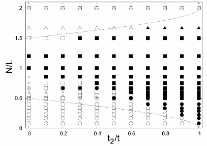
Figure 6: Magnetic phase diagram of the one-dimensional lateral lattice. The vertical axis shows the number of particles per site (on $p$-states) and the lateral axis the ratio $t_{2}/t$ of the two hopping parameters. The dashed lines show the borders between which the narrower band ($t_{2}$ band) is filled. Outside this area the lattice is antiferromagnetic (except at $t_{2}=t$). The filled (open) symbols show the ferromagnetic (antiferromagnetic) ground states obtained with exact diagonalization of the Hubbard Hamiltonian for 10 (triangles), 6 (squares), and 2 (circles) particles. Crosses show those results for $N=6$ which are not ferro or antiferromagnetic, i.e. $0<S<N/2$. The numerical results are for $U=10$.

Figure 6 shows the magnetism of the ground state, as a function of both the number of particles per site (on the $p$-states) and the ratio $t_{2}/t$ of the two hopping parameters, calculated by diagonalizing the Hubbard Hamiltonian. The figure also shows the limits given by Eqs. (6) and (7). Indeed, we see that between these limits, the ground state is mainly ferromagnetic, while outside these limits it is always antiferromagnetic. Figure 6 shows results computed for 2, 6 and 10 particles, where the ferromagnetic phase is simple and seen as the spin being at maximum $S=N/2$. As discussed above, for $N=4,~{}8,~{}12,~{}\cdots$ the ferromagnetic state has a spin-wave (or domains) and interpretation of the magnetic structure is more difficult. Nevertheless, results computed for those particle numbers seem to agree with the phase diagram shown in Fig. 6. The results in Fig. 6 are computed for $U=10$. We repeated some of the points for larger values of $U$ and found the same magnetic states.

It is interesting to compare the above results of the generalised Hubbard model with those of the density functional mean field theorykarkkainen2007 ; karkkainen2007a ; karkkainen2007b . The qualitative agreement is perfect: In the case of two $p$-particles per site ($N/L=2$) the system shows antiferromagnetism of spin-one quasiparticles, while in the case of one $p$ particle per site ($N/L=1$) the system is ferromagnetic. An even simpler tight-binding modelkoskinen2003 also gives a similar phase diagram. Due to the symmetry of the Hamiltonian, it is natural that also above the filling $N/L=2$ one obtains a ferromagnetic region with its center at $N/L=3$.

For small values of $t_{2}$ the corresponding single-particle band becomes very narrow. In this case the ferromagnetism can be understood with the Stoner mechnanismmattis1981 : The Fermi level is in the region of large density of states and induces a ferromagnetic state. In 1D this effect is particularly strong due to the singularities in the density of states karkkainen2007 .

IV Conclusions

We studied the magnetism of one-dimensional artificial lattices made of quasi-two-dimensional potential wells, for up to four particles per lattice site, i.e. in the region where the $1p$ level is filled. We froze the $1s$ particles and considered only the $1p$ states. Numerical diagonalization of a generalized Hubbard model was performed for several particle numbers and filling fractions. The results were analyzed using the antiferromagnetic Heisenberg model and single-particle models.

In the resulting phase diagram, the vertical lattice is ferromagnetic, except at a singular point with exactly two $p$-type particles per site. For lateral lattices the ground state is antiferromagnetic for small fillings and close to half-filling of the $p$-shell, but ferromagnetic around the region with one $p$-particle per site. A simple model for the ferromagnetic region was suggested.

If the particle number is a multiple of four ($N=4,8,~{}12,\cdots$), the ferromagnetic state has a spin wave which removes the degeneracy and yields a total spin $S=0$.

For polarized fermions the half-filled case shows “orbital antiferromagnetism” where in successive lattice sites the particles rotate clockwise and counter-clockwise.

Acknowledgments

This work was supported by the Academy of Finland and by the Jenny and Antti Wihuri Foundation, as well as NordForsk, the Swedish Research Council and the Swedish Foundation for Strategic Research.

References

- (1) H. Lee, J.A. Johnson, M.Y. He, J.S. Speck, and P.M. Petroff, Appl. Phys. Lett. 78, 105 (2001).
- (2) M. Schmidbauer, S. Seydmohamadi, D. Grigoriev, Z.M. Wang, Y.I. Mazur, P. Schafer, M. Hanke, R. Kohler, and G.J. Salamo, Phys. Rev. Lett. 96, 066108 (2006).
- (3) S. Kohmoto, H. Nakamura, S. Nishikawa, and K. Asakawa, Physica E 13, 1131 (2002).
- (4) Köhl, M. & Esslinger, T. Fermionic atoms in an optical lattice: a new synthetic material. Europhysics News 37, 18 (2006).
- (5) Jaksch, D. & Zoller, P. The cold atom Hubbard toolbox. Annals of Physics 315, 52 (2005).
- (6) M. Greiner, O. Mandel, T. Esslinger, T.W. Hänsch and I. Bloch, Nature 415, 39 (2002).
- (7) D.J. Han, S. Wolf, S. Oliver, C. McCormick, M. T. DePue, and D.S.Weiss, Phys. Rev. Lett. 85, 724 (2000).
- (8) A.J. Kerman, V. Vuletic, C. Chin, and S. Chu, Phys. Rev. Lett. 84, 439 (2000).
- (9) G. Modugno, F. Ferlaino, R. Heidemann, G. Roati, and M. Inguscio, Phys. Rev. A 68, 011601 (2003).
- (10) T. Rom, Th. Best, D. van Oosten, U. Schneider, S. Fölling, B. Paredes, and I. Bloch, Nature 444, 733 (2006).
- (11) J.K. Chin, D.E. Miller, Y. Liu, C. Stan, W. Setiawan, C. Sanner, K. Xu, and W. Ketterle, Nature 443, 961 (2006).
- (12) Feshbach, H. Unified Theory of Nuclear Reactions. Annals of Physics 5, 357 (1958).
- (13) Inouye, S. Observation of Feshbach resonances in a Bose-Einstein condensate. et al. Nature 392, 151 (1998).
- (14) Courteille, Ph. et al. Observation of a Feshbach Resonance in Cold Atom Scattering. Phys. Rev. Lett. 81, 69 (1998).
- (15) Roberts, J. L. et al. Resonant Magnetic Field Control of Elastic Scattering in Cold 85Rb. Phys. Rev. Lett. 81, 5109 (1998).
- (16) Duine, R. A. & Stoof, H. T. C. Atom-molecule coherence in Bose gases. Physics Reports 396, 115 (2004)
- (17) Theis, M. Tuning the Scattering Length with an Optically Induced Feshbach Resonance. Phys. Rev. Lett. 93, 123001 (2004)
- (18) S.-J. Gu, R. Fan, and H.-Q. Lin, lattice Phys. Rev. B 76, 125107 (2007).
- (19) G. Xianlong, M. Rizzi, Marco Polini, R. Fazio, M.P. Tosi, V.L. Campo, Jr., and K. Capelle, Phys. Rev. Lett. 98, 030404 (2007).
- (20) F. Massel and V. Penna, Phys. Rev. A 72, 053619 (2005).
- (21) T. Koponen, J. Kinnunen, J.P. Martikainen, L.M. Jensen, P. Törmä, New. J. Phys. 8, 179 (2006).
- (22) T.K. Koponen, T. Paananen, J.P. Martikainen, and P. Törmä, Phys. Rev. Lett. 99 120403 (2007).
- (23) H. Chen, J. Wu, Z.Q. Li, and Y. Kawazoe, insulator transition Phys. Rev. B 55, 1578 (1997).
- (24) M. Taut, between the dots Phys. Rev. B 62, 8126 (2000).
- (25) M. Koskinen, M. Manninen, and S.M. Reimann, Phys. Rev. Lett. 79, 1389 (1997).
- (26) S.M. Reimann and M. Manninen, Rev. Mod. Phys. 74, 1283 (2002).
- (27) M. Koskinen, S.M. Reimann, and M. Manninen, Phys. Rev. Lett. 90, 066802 (2003).
- (28) K. Karkkainen, M. Koskinen, S.M. Reimann, and M. Manninen, Phys. Rev. B 72, 165324 (2005).
- (29) K. Kärkkäinen, M. Borgh, M. Manninen, and S.M. Reimann, New J. Phys. 9, 33 (2007).
- (30) K. Kärkkäinen, M. Borgh, M. Manninen, and S.M. Reimann, Eur. Phys. J D 43, 225 (2007).
- (31) P. Koskinen, L. Sapienza, and M. Manninen, Physica Scripta 68, 74 (2003).
- (32) J.Kolehmainen, S.M. Reimann, M. Koskinen, and M. Manninen, Eur. Phys. J. B 13, 731 (2000).
- (33) C. Yannouleas and U. Landman, Phys. Rev. Lett. 82, 5325 (1999).
- (34) M. Bayer, P. Hawrylak, K. Hinzer, S. Fafard, M. Korkusinski, Z.R. Wasilewski, O. Stern, and A. Forchel, Science 291, 451 (2001).
- (35) A. Harju, S. Siljamaki S, and R.M. Nieminen, Phys. Rev. Lett. 88, 226804 (2002).
- (36) F. Mireles, S.E. Ulloa, F. Rojas, and E. Cota, Appl. Phys. Lett. 88, 093118 (2006).
- (37) M. Scheibner, M. F. Doty, I. V. Ponomarev, A. S. Bracker, E. A. Stinaff, V. L. Korenev, T. L. Reinecke, and D. Gammon, Phys. Rev. B 75, 245318 (2007).
- (38) W. Zhang, T. Dong, and A.O. Govorov, Phys. Rev. B 76, 075319 (2007).
- (39) J. Voit, Rep. Prog. Phys. 57, 977 (1994).
- (40) E.B. Kolomeisky, and J.P. Straley, Rev. Mod. Phys. 68, 175 (1996).
- (41) Jaksch, D., Brunder, C., Cirac, J. I., Gardiner, C. W. & Zoller, P. Cold Bosonic Atoms in Optical Lattices. Phys. Rev. Lett. 81, 3108 (1998).
- (42) Greiner, M., Mandel, O., Esslinger, T., Hänsch, T. W. & Bloch, I. Quantum phase transition from a superfluid to a Mott insulator in a gas of ultracold atoms. Nature 415, 39 (2002).
- (43) Stöferle, T., Moritz, H., Schori, C., Köhl, M. & Esslinger, T. Transition from a Strongly Interacting 1D Superfluid to a Mott Insulator. Phys. Rev. Lett. 92, 130403 (2004).
- (44) Xu, K. Sodium Bose-Einstein condensates in an optical lattice. Phys. Rev. A 72, 043604 (2005).
- (45) E.H. Lieb and F.Y. Wu, Phys. Rev. Lett. 20, 1445 (1968).
- (46) G.M. Pastor, R. Hirsch, and B. Mühlschleger, Phys. Rev. Lett. 72, 3879 (1994).
- (47) F. Lopez-Urias and G.M. Pastor, Phys. Rev. B 59 5223 (1999).
- (48) S. Viefers, P. Koskinen, P.S. Deo, and M. Manninen, Physica E 21, 1 (2004).
- (49) N.W. Ashcroft and N.D. Mermin, Solid State Physics (Saunders College, Philadelphia 1976).
- (50) N. Yu and M. Fowler, Phys. Rev. B 45 11795 (1992).
- (51) D.C. Mattis, Theory of Magnetism (Springer 1981).