Searching for Communities in Bipartite Networks

Abstract

Bipartite networks are a useful tool for representing and investigating interaction networks. We consider methods for identifying communities in bipartite networks. Intuitive notions of network community groups are made explicit using Newman’s modularity measure. A specialized version of the modularity, adapted to be appropriate for bipartite networks, is presented; a corresponding algorithm is described for identifying community groups through maximizing this measure. The algorithm is applied to networks derived from the EU Framework Programs on Research and Technological Development. Community groups identified are compared using information-theoretic methods.

1 Introduction

Networks have attracted a burst of attention in the last decade (useful reviews include Refs. Christensen and Albert (2007); Dorogovtsev and Mendes (2004); Newman (2003); Albert and Barabási (2002)), with applications to natural, social, and technological networks. Within biology, networks are prevalent, including: neural networks, where synapses link neurons; metabolic networks, describing metabolic processes in the cell, linking chemical reactions and the regulatory processes that control them; protein interaction networks, representing physical interactions between an organism’s proteins; transcription networks, describing regulatory interactions between different genes; food webs, using links to characterize who eats whom; and networks of sexual relations and infections, including AIDS models. Taking a broader view, networks seem to be everywhere! There are: electrical power grids, whose stability relates to the network structure; airline networks, with service efficiency tied to properties of the network; the World Wide Web, with search engines using the network links to locate pages; networks in linguistics, with words linked by co-occurrence; social networks of all sorts (Burt, 1992; Coulon, 2005; Granovetter, 1973); collaboration networks, describing joint works amongst actors, authors, research labs, …; and many more.

Of great current interest is the identification of community groups, or modules, within networks. Stated informally, a community group is a portion of the network whose members are more tightly linked to one another than to other members of the network. A variety of approaches (Angelini et al., 2007; Gol’dshtein and Koganov, 2006; Hastings, 2006; Newman and Leicht, 2007; Reichardt and Bornholdt, 2006; Palla et al., 2005; Newman and Girvan, 2004; Clauset et al., 2004; Girvan and Newman, 2002) have been taken to explore this concept; see Refs. Danon et al. (2005); Newman (2004a) for useful reviews. Detecting community groups allows quantitative investigation of relevant subnetworks. Properties of the subnetworks may differ from the aggregate properties of the network as a whole, e.g., modules in the World Wide Web are sets of topically related web pages.

Methods for identifying community groups can be specialized to distinct classes of networks, such as bipartite networks Barber (2007); Guimerà et al. (2007). The nodes in a bipartite network can be partitioned into two disjoint sets such that no two nodes within the same set are adjacent. Bipartite networks thus feature two distinct types of nodes, providing a natural representation for many affiliation or interaction networks, with one type of node representing actors and the other representing relations. Examples of actor-relation pairs include people attending events (Davis et al., 1941; Freeman, 2003; Doreian et al., 2004), court justices making decisions (Doreian et al., 2004), scientists jointly publishing articles (Newman, 2001a, b), organizations collaborating in projects (Barber et al., 2006; Roediger-Schluga and Barber, 2008), and legislators serving on committees (Porter et al., 2007). Arguably, bipartite networks are the empirically standard case for social networks and other interaction networks, with unipartite networks appearing—often implicitly—as projections.

2 Community Structure in Networks

2.1 A Few Words on Graphs

We formally describe networks using the language of graph theory. Let $V$ be a set of vertices and $E$ be a set of vertex pairs or edges from $V\times V$. The pair $G=\left(V,E\right)$ is called a graph. In a simple graph, all pairs $\left\{u,v\right\}\in E$ are distinct and $\left\{u,u\right\}\notin E$, i.e., there are no double lines or loops. Given a partition

$$V=V_{1}+V_{2}$$ (1)

where no edges exist between pairs of points within $V_{i}$, $i=1$ or $2$, then $G$ is said to be bipartite.

We shall consider simple graphs on a (large) finite set $V$:

$$V=\left\{1,2,\ldots,n\right\}\quad.$$ (2)

The number of edges or degree $d_{v}$ of vertex $v$ is defined by

$$d_{v}=\#\left(\left\{v,\cdot\right\}\in E\right)$$ (3)

The number of edges is

$$\left|E\right|=\frac{1}{2}\sum_{k=1}^{n}d_{k}\quad.$$ (4)

$2\left|E\right|$ is often called the volume of the graph $G$.

Graph structure is encoded in the adjacency matrix

$$\mathbf{A}=\left(A_{ik}\right)_{1\leq i,k\leq n}\quad,$$ (5)

with

$$A_{ik}=\left\{\begin{array}[]{ll}1&\mbox{if }\left\{i,k\right\}\in E\\ 0&\mbox{otherwise}\end{array}\right.\quad.$$ (6)

2.2 Modularity

Detecting community groups allows for the identification and quantitative investigation of relevant subnetworks. Local properties of the community groups may differ from the global properties of the complete network. For example, topically related web pages in the World Wide Web are typically interlinked, so that the contents of pages in distinct community groups should reveal distinct themes. Thus, identification of community groups within a network is a first step towards understanding the heterogeneous substructures of the network.

To identify communities, we take as our starting point the modularity, introduced by Newman and Girvan (2004). Modularity makes intuitive notions of community groups precise by comparing network edges to those of a null model. As noted by Newman (2006):

A good division of a network into communities is not merely one in which there are few edges between communities; it is one in which there are fewer than expected edges between communities.

Definition 1

The modularity $Q$ is—up to a normalization constant—the number of edges within communities $c$ minus those for a null model:

$$Q\equiv\frac{1}{2\left|E\right|}\sum_{c}\sum_{i,j\in c}\left(A_{ij}-P_{ij}\right)\quad.$$ (7)

Along with eq. (7), it is necessary to provide a null model, defining $P_{ij}$. The standard choice for the null model constrains the degree distribution for the vertices to match the degree distribution in the actual network. Random graph models of this sort are obtained (Chung and Lu, 2002) by putting an edge between vertices $i$ and $j$ at random, with the constraint that on average the degree of any vertex $i$ is $d_{i}$. This constrains the expected adjacency matrix such that

$$d_{i}=E\left(\sum_{j}A_{ij}\right)\quad.$$ (8)

Denote $E\left(A_{ij}\right)$ by $P_{ij}$ and assume further that $P$ factorizes into

$$P_{ij}=p_{i}p_{j}\quad,$$ (9)

leading to

$$P_{ij}\equiv\frac{d_{i}d_{j}}{2\left|E\right|}\quad.$$ (10)

A consequence of the null model choice is that $Q=0$ when all vertices are in the same community.

The goal now is to find a division of the vertices into communities such that the modularity $Q$ is maximal. An exhaustive search for a decomposition is out of the question: even for moderately large graphs there are far too many ways to decompose them into communities. Fast approximate algorithms do exist (see, for example, Refs. (Pujol et al., 2006; Newman, 2004b)).

2.3 Finding Communities with BRIM

Specific classes of networks have additional constraints that can be reflected in the null model. For bipartite graphs, the null model should be modified to reproduce the characteristic form of bipartite adjacency matrices

$$\mathbf{A}=\left[\begin{array}[]{cc}\mathbf{O}&\mathbf{M}\\ \mathbf{M}^{\mathrm{T}}&\mathbf{O}\end{array}\right]\quad.$$ (11)

Recently, specialized modularity measures and search algorithms have been proposed for finding communities in bipartite networks (Barber, 2007; Guimerà et al., 2007).

We make use of the algorithm called BRIM: bipartite, recursively induced modules (Barber, 2007). Starting from a (more or less) ad hoc partition of the vertices of type 1, it is straightforward to optimize a corresponding decomposition of the vertices of type 2. From there, optimize the decomposition of vertices of type 1, and iterate. In this fashion, modularity increases until a (local) maximum is reached. However, the question remains: is the maximum a “good” one? At this level then a random search is called for, varying the composition and number of communities, with the goal of reaching a better maximum after a new round of hill climbing using the BRIM algorithm.

3 An Initial Look at EU Research Networks

In the ongoing research project NEMO (nem, ????), networks of research and development collaborations under EU Framework Programs FP1, FP2,…, FP5 are studied. The collaborations in the Framework Programs give rise to bipartite graphs, with edges existing between projects and the organizations which take part in them. With this construction, participating organizations are linked only through joint projects.

In the various Framework Programs, the number of organizations ranges from 2,000 to 20,000, the number of projects ranges from 3,000 to 15,000, and the number of links between them (project participations) ranges from 10,000 to 250,000 (see table 1 for precise values). A popular approach in social network analysis—where networks are often small, consisting of a few dozen nodes—is to visualize the networks and identify community groups by eye. However, the Framework Program networks are much larger: can we “see” the community groups in these networks?

Framework Program	Period	Projects	Organizations
FP1	1984–1987	3,283	1,981
FP2	1987–1981	3,885	4,572
FP3	1990–1994	5,529	7,324
FP4	1994–1998	15,061	19,755
FP5	1998–2002	15,559	22,303

Table 1: R&D projects and participants in the EU Framework Programs. The projects and organizations are used to define bipartite networks for each of the Framework Programs.

Structural differences or similarities of such networks are not obvious at a glance. For a graphical representation of the organizations and/or projects by dots on an A4 sheet of paper, we would have to put these dots at a distance of about $1\,\mathrm{mm}$ from each other, and we then still would not have drawn the links (collaborations) which connect them.

Previous studies used a list of coarse graining recipes to compact the networks into a form which would lend itself to a graphical representation Breschi and Cusmano (2004). As an alternative we have attempted to detect communities just using BRIM, i.e., purely on the basis of relational network structure, and blind with respect to any additional information about the nature of agents.

In Fig. 1, we show a community structure for FP3 found using the BRIM algorithm, with a modularity of $Q=0.602$ for 14 community groups. The communities are shown as vertices in a network, with the vertex positions determined using spectral methods (Seary and Richards, 2003). The area of each vertex is proportional to the number of edges from the original network within the corresponding community. The width of each edge in the community network is proportional to the number of edges in the original network connecting community members from the two linked groups. The vertices and edges are shaded to provide additional information about their topical structure, as described in the next section. Each community is labeled with the most frequently occurring subject index.

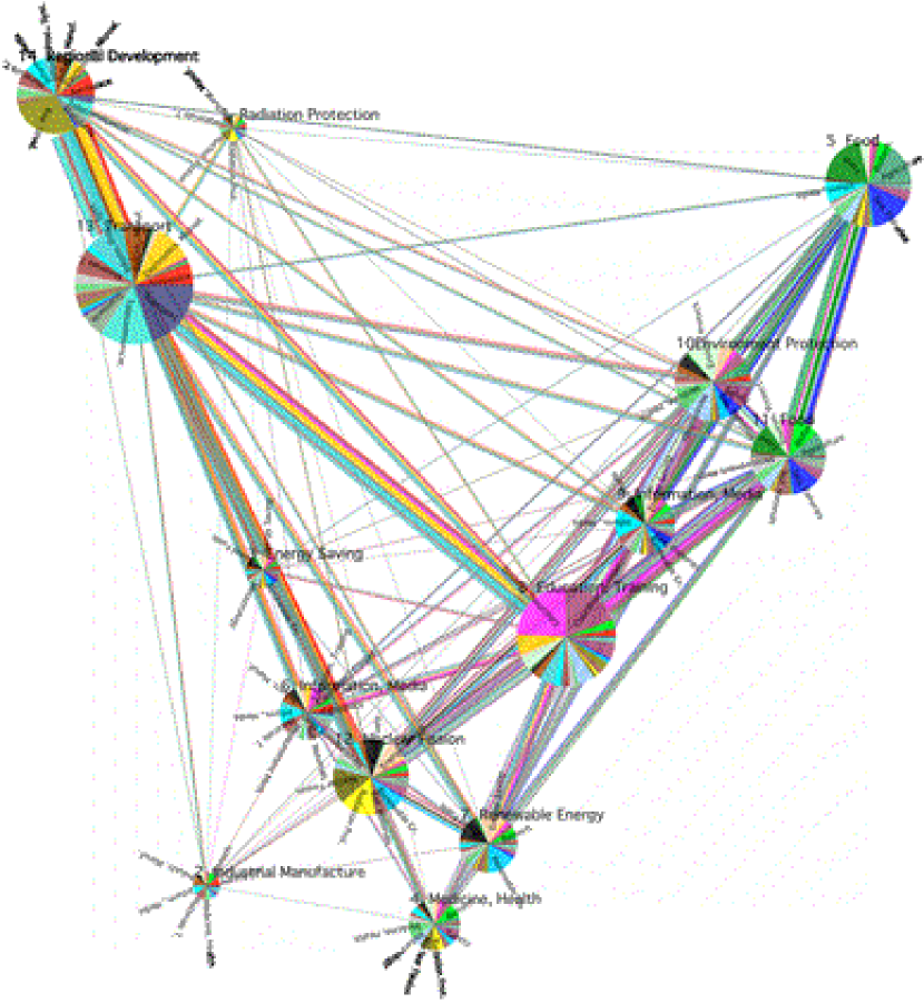
Figure 1: Community groups in the network of projects and organizations for FP3.

3.1 Topical Profiles of Communities

Projects are assigned one or more standardized subject indices. There are 49 subject indices in total, ranging from Aerospace to Waste Management.

We denote by

$$f\left(t\right)>0$$ (12)

the frequency of occurrence of the subject index $t$ in the network, with

$$\sum\limits_{t}f\left(t\right)=1\quad.$$ (13)

Similarly we consider the projects within one community $c$ and the frequency

$$f_{c}\left(t\right)\geq 0$$ (14)

of any subject index $t$ appearing in the projects only of that community. We call $f_{c}$ the topical profile of community $c$ to be compared with that of the network as a whole.

Topical differentiation of communities can be measured by comparing their profiles, among each other or with respect to the overall network. This can be done in a variety of ways (Gibbs and Su, 2002), such as by the Kullback “distance”

$$D_{c}=\sum\limits_{t}f_{c}\left(t\right)\ln\frac{f_{c}\left(t\right)}{f\left(t\right)}\quad.$$ (15)

A true metric is given by

$$d_{c}=\sum\limits_{t}\left|f_{c}\left(t\right)-f\left(t\right)\right|\quad,$$ (16)

ranging from zero to two.

Topical differentiation is illustrated in Fig. 2. In the figure, example profiles are shown, taken from the network in Fig. 1. The community-specific profile corresponds to the community labeled ‘11. Food” in Fig. 1. Based on the most frequently occurring subject indices—Agriculture, Food, and Resources of the Seas, Fisheries—the community consists of projects and organizations focussed on R&D related to food products. The topical differentiation is $d_{c}=0.90$ for the community shown.

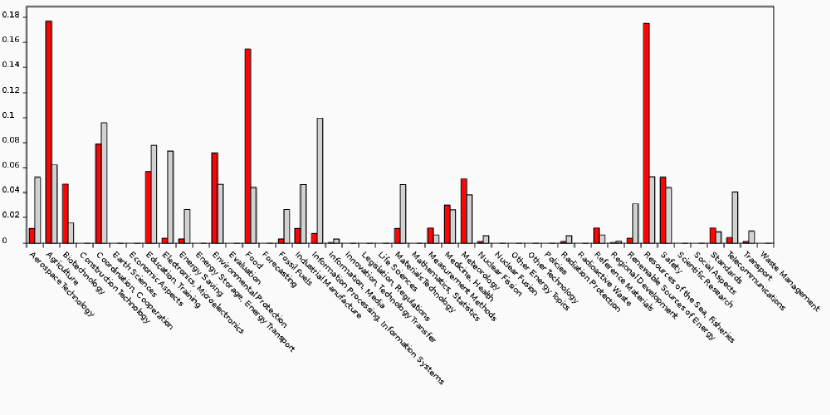
Figure 2: Topical differentiation in a network community. The histogram shows the difference between the topical profile $f_{c}\left(t\right)$ for a specific community (dark bars) and the overall profile $f\left(t\right)$ for the network as a whole (light bars). The community-specific profile shown is for the community labeled “11. Food” in Fig. 1. The community has $d_{c}=0.90$.

3.2 Projects and Subject Indices

For further analysis, we have also looked for communities in networks of projects and subject indices. Here, the projects and subject indices constitute the vertices of a bipartite network, with edges existing between projects and the subject indices assigned to them. This construction disregards the organizations, providing an alternate approach to investigating the topical structure of the Framework Programs.

In Fig. 3, we show a set of nine community groups identified for the network of projects and subject indices in FP5. The modularity is $Q=0.50290$ with these community groups.

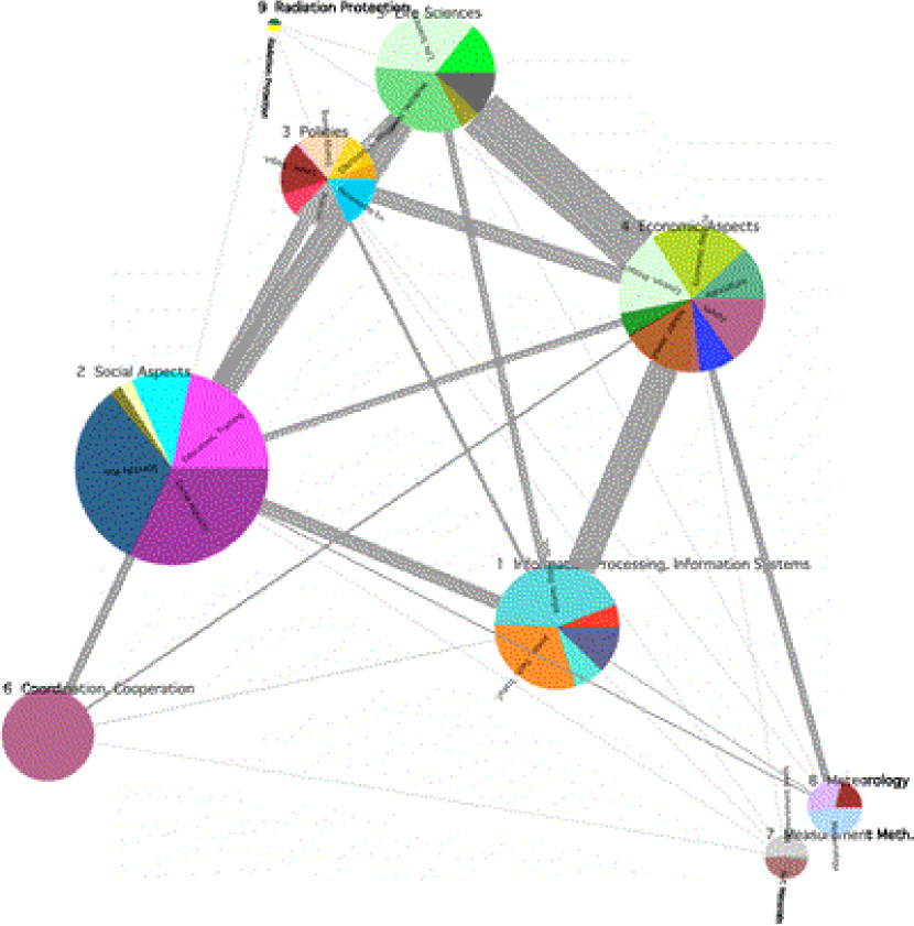
Figure 3: Community groups in the network of projects and subject indices for FP5.

The later Framework Programs, such as FP5, show a fair degree of overlap between the communities, due to the subject indices being freely assigned in project applications. This is in marked contrast to the networks for the first three Framework Programs, where topics were attributed rigidly within thematic subprograms. The communities for FP1–3 thus have more clearly segregated community structures. FP1 is particularly extreme, having no overlaps between the communities. The differences between Framework Programs point to the need for some care in interpreting community structures: the communities in FP1–3 reflect policy structures while those found for later Framework Programs are more representative of interaction patterns.

3.3 Comparing Decompositions with the Mutual Information

For different decompositions of a (finite) set $\Omega$, a measure of similarity is provided by the normalized mutual information (Danon et al., 2005). Set

$$p(A)=\frac{\left|A\right|}{\left|\Omega\right|}\quad.$$ (17)

For divisions of $\Omega$ into

1. J disjoint subsets $X_{1},\ldots,X_{J}$ and

2. K disjoint subsets $Y_{1},\ldots,Y_{K}$,

compute the mutual information

$$I_{0}(X,Y)=\sum\limits_{jk}p\left(X_{j}\cap Y_{k}\right)\log\frac{p\left(X_{j}\cap Y_{k}\right)}{p\left(X_{j}\right)p\left(Y_{k}\right)}$$ (18)

and normalize

$$I(X,Y)=\frac{2I(X,Y)}{H(X)+H(Y)}\quad,$$ (19)

where the entropy $H$ is

$$H(X)=-\sum_{j}p\left(X_{j}\right)\log p\left(X_{j}\right)\quad.$$ (20)

With the definitions in eqs. (18) through (20), $I$ ranges from zero, for uncorrelated decompositions of the set, to one, for perfectly correlated decompositions.

Using the BRIM algorithm, we have partitioned network vertices into community groups by maximizing the modularity $Q$. In principle, many dissimilar partitions of the vertices could produce similar modularity values. With the normalized mutual information (or a similar measure), we can assess the amount of shared structure between two different partitions of the vertex set.

For example, in Fig. 3 we have shown a decomposition of the network of projects and subject indices for FP5. In Fig. 4, we show a second decomposition of the same network. The modularity is nearly identical—$0.50296$ instead of the $Q=0.50290$ seen previously—and the decompositions have some visible similarities. However, there are also definite structural differences, most prominently that the second decomposition has only eight communities while the first has nine. Are the structural differences significant? The normalized mutual information is found to be $I=0.98$, indicating a strong correlation between the two decompositions and demonstrating that they have relatively minor structural differences.

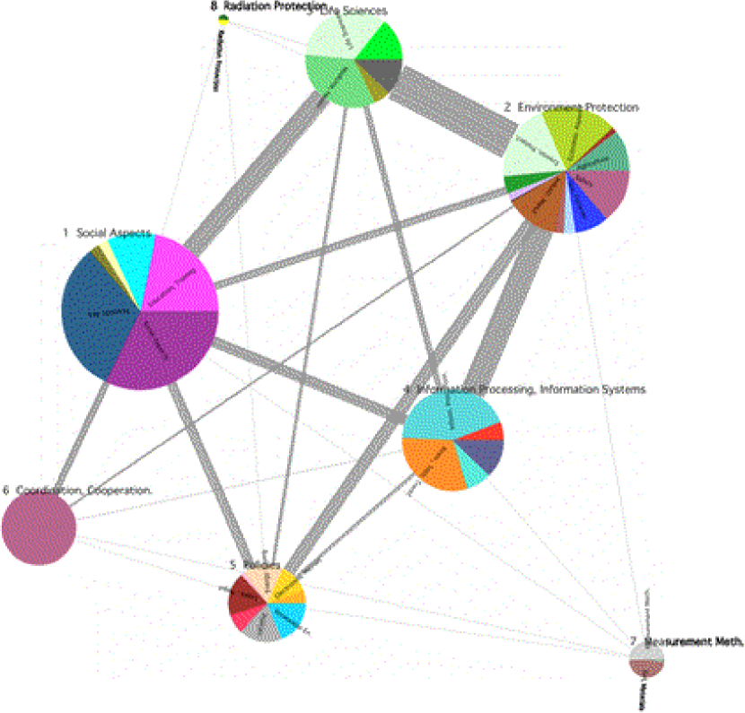
Figure 4: An alternate set of community groups in the network of projects and subject indices for FP5.

3.4 Outlook

We have successfully identified community groups in networks defined from the Framework Program projects and the subject indices assigned to them. The full networks defined from the projects and the organizations taking part in them are considerably larger and correspondingly more challenging to investigate. For the full organizations-projects network, the BRIM hill climbing algorithm is being supplemented with an aggressive, probabilistic search through community configurations upon which BRIM acts. This extended search has only just begun, but preliminary results are encouraging.

Once established, communities will then be investigated with regard to their internal structure, with the goal of identifying correlated properties within communities and contrasting properties across communities. We expect the analysis of internal structure to reveal patterns, themes, and motivations of collaborative research and development in the European Union.

References

- Christensen and Albert (2007) C. Christensen, and R. Albert, International Journal of Bifurcation and Chaos 17, 2201–2214 (2007), URL http://arxiv.org/abs/q-bio.OT/0609036, special Issue “Complex Networks’ Structure and Dynamics”.
- Dorogovtsev and Mendes (2004) S. N. Dorogovtsev, and J. F. F. Mendes, “The shortest path to complex networks,” in Complex Systems and Inter-disciplinary Science, edited by N. Johnson, J. Efstathiou, and F. Reed-Tsochas, World Scientific, 2004, URL http://arxiv.org/abs/cond-mat/0404593.
- Newman (2003) M. E. J. Newman, SIAM Review 45, 167–256 (2003), URL http://arxiv.org/abs/cond-mat/0303516.
- Albert and Barabási (2002) R. Albert, and A.-L. Barabási, Reviews of Modern Physics 74, 47 (2002), URL http://link.aps.org/abstract/RMP/v74/p47.
- Burt (1992) R. S. Burt, Structural Holes: The Social Structure of Competition, Harvard University Press, Cambridge, MA, 1992.
- Coulon (2005) F. Coulon, The use of social network analysis in innovation research: A literature review, Danish Research Unit for Industrial Dynamics (2005).
- Granovetter (1973) M. Granovetter, The American Journal of Sociology 78, 1360–1380 (1973).
- Angelini et al. (2007) L. Angelini, S. Boccaletti, D. Marinazzo, M. Pellicoro, and S. Stramaglia, Chaos: An Interdisciplinary Journal of Nonlinear Science 17, 023114 (2007), URL http://arxiv.org/abs/cond-mat/0610182.
- Gol’dshtein and Koganov (2006) V. Gol’dshtein, and G. A. Koganov, An indicator for community structure (2006), URL http://arxiv.org/abs/physics/0607159, preprint.
- Hastings (2006) M. B. Hastings, Physical Review E (Statistical, Nonlinear, and Soft Matter Physics) 74, 035102 (2006), URL http://arxiv.org/abs/cond-mat/0604429.
- Newman and Leicht (2007) M. E. J. Newman, and E. A. Leicht, PNAS 104, 9564–9569 (2007), URL http://www.pnas.org/cgi/content/abstract/104/23/9564, http://arxiv.org/abs/physics/0611158/.
- Reichardt and Bornholdt (2006) J. Reichardt, and S. Bornholdt, Physical Review E (Statistical, Nonlinear, and Soft Matter Physics) 74, 016110 (2006), URL http://link.aps.org/abstract/PRE/v74/e016110, cond-mat/0603718.
- Palla et al. (2005) G. Palla, I. Derenyi, I. Farkas, and T. Vicsek, Nature 435, 814–818 (2005), URL http://arxiv.org/abs/physics/0506133.
- Newman and Girvan (2004) M. E. J. Newman, and M. Girvan, Physical Review E (Statistical, Nonlinear, and Soft Matter Physics) 69, 026113 (2004), URL http://link.aps.org/abstract/PRE/v69/e026113.
- Clauset et al. (2004) A. Clauset, M. E. J. Newman, and C. Moore, Physical Review E (Statistical, Nonlinear, and Soft Matter Physics) 70, 066111 (2004), URL http://link.aps.org/abstract/PRE/v70/e066111.
- Girvan and Newman (2002) M. Girvan, and M. E. J. Newman, PNAS 99, 7821–7826 (2002), URL http://www.pnas.org/cgi/content/abstract/99/12/7821, http://www.pnas.org/cgi/reprint/99/12/7821.pdf.
- Danon et al. (2005) L. Danon, A. Díaz-Guilera, J. Duch, and A. Arenas, J. Stat. Mech. P09008 (2005), URL http://www.iop.org/EJ/article/1742-5468/2005/09/P09008/jstat5%_09_p09008.html.
- Newman (2004a) M. E. J. Newman, Eur. Phys. J. B 38, 321–330 (2004a), URL http://www-personal.umich.edu/~mejn/papers/epjb.pdf.
- Barber (2007) M. J. Barber, Physical Review E (Statistical, Nonlinear, and Soft Matter Physics) 76, 066102 (2007), URL http://arxiv.org/abs/0707.1616, arXiv:0707.1616.
- Guimerà et al. (2007) R. Guimerà, M. Sales-Pardo, and L. A. N. Amaral, Physical Review E (Statistical, Nonlinear, and Soft Matter Physics) 76, 036102 (2007), URL http://link.aps.org/abstract/PRE/v76/e036102.
- Davis et al. (1941) A. Davis, B. B. Gardner, and M. R. Gardner, Deep South, University of Chicago Press, 1941.
- Freeman (2003) L. Freeman, “Finding social groups: A meta-analysis of the southern women data,” in Dynamic Social Network Modeling and Analysis, edited by R. Breiger, K. Carley, and P. Pattison, The National Academies Press, Washington, DC, 2003, URL http://moreno.ss.uci.edu/85.pdf.
- Doreian et al. (2004) P. Doreian, V. Batagelj, and A. Ferligoj, Social Networks 26, 29–53 (2004).
- Newman (2001a) M. E. J. Newman, Physical Review E (Statistical, Nonlinear, and Soft Matter Physics) 64, M. E. J. Newman (2001a), URL http://www-personal.umich.edu/~mejn/papers/016131.pdf.
- Newman (2001b) M. E. J. Newman, Physical Review E (Statistical, Nonlinear, and Soft Matter Physics) 64, 016132 (2001b), URL http://www-personal.umich.edu/~mejn/papers/016132.pdf.
- Barber et al. (2006) M. J. Barber, A. Krueger, T. Krueger, and T. Roediger-Schluga, Physical Review E (Statistical, Nonlinear, and Soft Matter Physics) 73, 036132 (2006), URL http://link.aps.org/abstract/PRE/v73/e036132.
- Roediger-Schluga and Barber (2008) T. Roediger-Schluga, and M. J. Barber, IJFIP 4, 321–347 (2008), special Issue on “Innovation Networks”.
- Porter et al. (2007) M. A. Porter, P. J. Mucha, M. E. J. Newman, and A. J. Friend, Physica A 386, 414–438 (2007), URL http://arxiv.org/abs/physics/0602033.
- Newman (2006) M. E. J. Newman, Proceedings of the National Academy of Sciences 103, 8577–8582 (2006), URL http://www.pnas.org/cgi/content/abstract/103/23/8577.
- Chung and Lu (2002) F. Chung, and L. Lu, Annals of Combinatorics 6, 125–145 (2002).
- Pujol et al. (2006) J. M. Pujol, J. Bejar, and J. Delgado, Physical Review E (Statistical, Nonlinear, and Soft Matter Physics) 74, 016107 (2006), URL http://link.aps.org/abstract/PRE/v74/e016107.
- Newman (2004b) M. E. J. Newman, Physical Review E (Statistical, Nonlinear, and Soft Matter Physics) 69, 066133 (2004b), URL http://link.aps.org/abstract/PRE/v69/e066133.
- nem (????) NEMO: Network models, governance and R&D collaboration networks (????), URL http://www.nemo-net.eu.
- Breschi and Cusmano (2004) S. Breschi, and L. Cusmano, International Journal of Technology Management 27, 747–72 (2004).
- Seary and Richards (2003) A. J. Seary, and W. D. Richards, “Spectral methods for analyzing and visualizing networks: an introduction,” in Dynamic Social Network Modeling and Analysis: Workshop Summary and Papers, edited by R. Breiger, K. Carley, and P. Pattison, The National Academies Press, Washington, D.C., 2003, pp. 209–228, URL http://www.sfu.ca/~richards/Pages/NAS.AJS-WDR.pdf.
- Gibbs and Su (2002) A. Gibbs, and F. Su, International Statistical Review 70, 419–435 (2002).